Equivalent block transmissivity in an irregular 2D polygonal grid for one-phase flow: A sensitivity analysis

Marco De Lucia; Chantal de Fouquet; Vincent Lagneau; Roberto Bruno

doi:10.1016/j.crte.2008.11.014

Surface geosciences (hydrology-hydrogeology)

Equivalent block transmissivity in an irregular 2D polygonal grid for one-phase flow: A sensitivity analysis
[Calcul de la transmissivité de bloc en maillage polygonal irrégulier 2D pour un écoulement monophasique : une étude de sensibilité]

Présenté par : Ghislain de Marsily

Marco De Lucia ^1,² ; Chantal de Fouquet ¹ ; Vincent Lagneau ¹ ; Roberto Bruno ²

¹ Mines ParisTech, centre de géosciences, 35, rue Saint-Honoré, 77305 Fontainebleau cedex, France
² Università di Bologna, Dipartimento di Ingegneria Chimica, Mineraria e delle Tecnologie Ambientali, Via Terracini, 28, 40131 Bologna, Italy

Comptes Rendus. Géoscience, Volume 341 (2009) no. 4, pp. 327-338.

Résumés

Anglais
Français

Upscaling is needed to transform the representation of non-additive space-dependent variables, such as permeability, from the fine grid of geostatistical simulations (to simulate small-scale spatial variability) to the coarser, generally irregular grids for hydrodynamic transport codes. A new renormalisation method is proposed, based on the geometric properties of a Voronï grid. It is compared to other classic methods by a sensitivity analysis (grid, range and sill of the variogram, random realisation of a simulation); the criterion is the flux of a tracer at the outlet. The effect of the upscaling technique on the results appears to be of second order compared to the spatial discretisation, the choice of variogram, and the realisation.

Le changement d’échelle pour la perméabilité est incontournable, entre une simulation géostatistique sur grille fine (reproduisant la variabilité spatiale à petite distance) et le maillage plus grossier et généralement irrégulier des codes de transport. Une nouvelle méthode de renormalisation, exploitant les propriétés géométriques du maillage de Voronï, est comparée à deux méthodes classiques, par une étude de sensibilité (maillage, portée et palier du variogramme, tirage ou « réalisation » d’une simulation) suivant un critère de flux d’un traceur en sortie de perméamètre. La technique de changement d’échelle apparaît du second ordre par rapport à la discrétisation spatiale, au variogramme et à la réalisation.

Métadonnées

Reçu le : 2007-12-20
Accepté le : 2008-11-04
Publié le : 2009-04-01

DOI : 10.1016/j.crte.2008.11.014

Keywords: Equivalent permeability, Upscaling, Finite volumes, Voronï mesh, Spatial variability, Heterogeneous medium, Flow
Mot clés : Perméabilité équivalente, Changement d’échelle, Volumes finis, Maillage de Voronï, Variabilité spatiale, Milieu hétérogène, Écoulement

Affiliations des auteurs :

Marco De Lucia ^{1, 2} ; Chantal de Fouquet ¹ ; Vincent Lagneau ¹ ; Roberto Bruno ²

@article{CRGEOS_2009__341_4_327_0,
     author = {Marco De Lucia and Chantal de Fouquet and Vincent Lagneau and Roberto Bruno},
     title = {Equivalent block transmissivity in an irregular {2D} polygonal grid for one-phase flow: {A} sensitivity analysis},
     journal = {Comptes Rendus. G\'eoscience},
     pages = {327--338},
     publisher = {Elsevier},
     volume = {341},
     number = {4},
     year = {2009},
     doi = {10.1016/j.crte.2008.11.014},
     language = {en},
}

TY  - JOUR
AU  - Marco De Lucia
AU  - Chantal de Fouquet
AU  - Vincent Lagneau
AU  - Roberto Bruno
TI  - Equivalent block transmissivity in an irregular 2D polygonal grid for one-phase flow: A sensitivity analysis
JO  - Comptes Rendus. Géoscience
PY  - 2009
SP  - 327
EP  - 338
VL  - 341
IS  - 4
PB  - Elsevier
DO  - 10.1016/j.crte.2008.11.014
LA  - en
ID  - CRGEOS_2009__341_4_327_0
ER  -

%0 Journal Article
%A Marco De Lucia
%A Chantal de Fouquet
%A Vincent Lagneau
%A Roberto Bruno
%T Equivalent block transmissivity in an irregular 2D polygonal grid for one-phase flow: A sensitivity analysis
%J Comptes Rendus. Géoscience
%D 2009
%P 327-338
%V 341
%N 4
%I Elsevier
%R 10.1016/j.crte.2008.11.014
%G en
%F CRGEOS_2009__341_4_327_0

Marco De Lucia; Chantal de Fouquet; Vincent Lagneau; Roberto Bruno. Equivalent block transmissivity in an irregular 2D polygonal grid for one-phase flow: A sensitivity analysis. Comptes Rendus. Géoscience, Volume 341 (2009) no. 4, pp. 327-338. doi : 10.1016/j.crte.2008.11.014. https://comptes-rendus.academie-sciences.fr/geoscience/articles/10.1016/j.crte.2008.11.014/

Version originale du texte intégral

1 Introduction

Upscaling is a required step to adapt a fine grid geostatistical simulation (to reproduce spatial variability at a different scale) to equivalent parameters on (usually irregular) grids used by transport codes. A new renormalisation method is proposed, based on the properties of a Voronï grid used in the code Hytec, to compute the inter-block permeability; this method does not require the knowledge of the local flow direction. Our computation of the scalar block permeability is compared to two other classical renormalisation methods, based on a parametric sensitivity analysis to the spatial variability, in two dimensions. The chosen observable is the cumulative flux of a non-reactive tracer through the outlet of the domain.

2 Bibliographical elements

Since the Renard and de Marsily synthesis [19], developments on upscaling methods are still carried out, in various domains: multiphase flow [6], fractured media [10,11,21], reactive transport [14], etc. Two general classes of methods can be highlighted:

• on the one hand cell aggregation, which aims at adapting the grid to the medium properties and the flow boundary conditions [1,3,12];
• on the other hand, methods which aim at attributing equivalent values (or at least an interval) for properties on a fixed geometry.

The second seems better adapted for numerical models with a high spatial variability [7], particularly when permeability or transmissivity are obtained by geostatistical simulations based on the anamorphosed Gaussian model. Furthermore, for reactive transport applications, the possible evolution of the pore structure, due to precipitation or dissolution reactions, is still a serious limitation to the use of adaptive grids.

2.1 Block permeability: exact results or inequalities

The equivalent permeability of a block is precisely known in a few particular cases [16]. According to the fundamental inequality, a block permeability is bounded by the harmonic- and the arithmetic-mean of its elements. When the permeability is simulated on a fine grid, the interval can become very large, if the blocks are constituted of numerous fine cell elements, or if the dispersion variance of the permeability of the cells inside the block is high. Several authors suggested tighter bounds, for particular media or boundary conditions [18]. For instance, for relatively general conditions (linear pressure or constant flux on the boundary), Pouya [17] shows the rise of two particular tensors, linked by an inequality: equivalent permeabilities in the direction of the mean gradient and the mean flux respectively. He then proposes to use these tensors as upper and lower bounds for the results, according to the problem to solve. While bounding the result is more rigourous, “realistic” values are sometimes sufficient, particularly when the computation times are large as in reactive transport.

2.2 Empirical formulas

For lack of a general rule for permeability composition, several empirical formulas have been studied, notably renormalisation methods: iterative treatments to remove small scale fluctuations [8]. In the following, we retain two expressions of block permeability.

The first one is based on Matheron's formula [16], a composition of the arithmetic mean μ_a and the harmonic mean μ_h, as a function of the dimension D of the space:

K_{M} = {(μ_{a})}^{α} {(μ_{h})}^{1 - α}

(1)

where

α = \frac{D - 1}{D}

. In dimension 2,

K_{M} = \sqrt{μ_{a} \cdot μ_{h}}

so that the equivalent transmissivity is the geometric mean of the harmonic and the arithmetic means of the transmissivities of the cells inside the block. This formula has since been generalised, e.g., [2,4].

The second method is based on the simplified renormalisation by Renard and Renard et al. [18,20]: it consists in an iterative composition of the values of the elementary cells contained by the block, alternating arithmetic and harmonic means. This method yields two bounds, following each axis of the grid: the lower (c_min) and upper (c_min) bounds are obtained when the first iteration uses a harmonic and an arithmetic mean, respectively. These bounds are then composed by power-average, taking into account the medium anisotropy if needed. Let u be the assumed direction of the tensor, taken parallel to one of the axes for simplicity; let $c_{min}^{u}$ and $c_{max}^{u}$ be the associated lower and upper bounds, respectively; let K^u be the diagonal component of the permeability tensor on the elementary cell in this direction. Then, for a 2D isotropic medium, the simplified renormalisation is the geometric mean of the two bounds given by the alternating means:

K_{S R}^{u} = \sqrt{c_{\max}^{u} \cdot c_{\min}^{u}}

(2)

This relationship is similar to Matheron's formula, but applies with tighter bounds. For an anisotropic medium, the upscaling transforms a scalar permeability into a tensorial permeability. If the flow solver accepts scalar values only, the block permeability can be computed by assuming the direction of the head gradient to be known. In 2D, for a diagonal permeability tensor in the directions (Ox,Oy), the permeability along the flow direction $\vec{s} = (\cos θ, \sin θ)$ is:

K_{R S} = \cos θ \cdot K_{S R}^{X} + \sin θ \cdot K_{S R}^{Y}

When the local direction of the flow $\vec{s}$ is not known, the consistency of the equivalent permeability obtained by this method decreases when the effective direction of $\vec{s}$ diverges from its supposed direction.

3 Irregular grid renormalisation

In his Ph.D thesis, Renard extends the simplified renormalisation to irregular blocks, by weighting the successive means depending on the blocks geometry ([18], p. 92–93). In the following, we investigate the transmissivity composition for a 2D medium, discretised by an irregular grid. While we work in the plane, we still use the term “permeability”: this is consistent, e.g., with a flow in a constant depth aquifer. The flow code is briefly introduced, then a new upscaling method is proposed, based on the specific properties of the spatial discretisation scheme.

3.1 The Hytec code: finite volumes on a Voronï polygons grid

Hytec [13,14] is a coupled hydrodynamic and geochemistry code. It is based on the resolution of the macroscopic equations of flow and advective/dispersive transport on a finite volumes scheme (or integrated finite differences), using a spatial discretisation by irregular Voronï polygons. The convex polygons are built, starting from an arbitrary set of points, by intersection of the perpendicular bisector of each pair of nodes. In a finite volumes formulation, all parameters are considered uniform inside each polygon.

For a one-phase stationary flow, Hytec solves the diffusivity equation and the associated Darcy's equation [15]:

\{\begin{array}{l} 0 = div (K \cdot \vec{grad} h) \\ \vec{U} = - K \cdot \vec{grad} h \end{array}

where h is the head (in m),

\vec{U}

is the Darcy velocity vector (in m/s), and K the permeability (in m/s). The equation is resolved with respect to the unknown h; then the normal component of

\vec{U}

is computed, on each cell boundary, via Darcy's equation. Once determined the flow velocity field, the transport equation is written:

\frac{\partial ω c}{\partial t} = div ((D_{e} + α ∥\vec{U}∥) \cdot \vec{grad} c - c \cdot \vec{U})

where ω is the porosity, c is the tracer concentration, D_e is the effective diffusion coefficient (in m²/s) and α the dispersivity (in m).

Hytec proposes a choice of algorithms for the resolution of the transport equation. The time and space interpolations are one-step, but the centring can be configured by the user. We chose for this study a time-centred pattern (Crank–Nicholson scheme), which has little effect on the result apart from the maximum admissible time step.

As to the space discretisation, Hytec proposes both an upward and a centred scheme. The first is unconditionally stable, but creates a numerical dispersion term (mathematically equivalent to a physical dispersivity α), locally of the order of a half-cell diameter. The second scheme is space-centred: it does not create numerical dispersion, but its stability is conditional on the local value of α. The first scheme is generally preferred for coupled reactive transport problems: indeed, the geochemistry usually limits the effects of dispersion by a chemical sharpening of the fronts. However, the numerical dispersion is proportional to the (local) size of the cells, so that an accurate comparison between several grid computations is difficult. The effects of the space centring are discussed further in the results, section 5.

3.2 Simplified renormalisation for a polygonal cell (Fig. 1)

The simplified renormalisation algorithm can be readily adapted to an irregular mesh, by weighting the means at each iteration according to the actual number of cells inside the polygon. This is indeed a local algorithm.

Fig. 1
Simplified renormalisation on a polygonal cell. When the flow direction is known a priori, the renormalisation is performed on the circum-rectangle, with weighting according to the relative surface of the blocks inside the polygon.
Fig. 1. Renormalisation simplifiée sur maille polygonale. La direction du flux étant fixée a priori, on procède à la renormalisation sur le rectangle qui contient le polygone, en pondérant les moyennes par la surface relative des blocs qui recouvrent le polygone.

In the following, a “cell” will refer to the fine regular mesh of the geostatistical simulation. The simplified renormalisation algorithm on an irregular mesh is then as follow (see Fig. 1):

1. each polygonal mesh is discretised into cells, following the circum-rectangle of the polygon;
2. a weight 1 is attributed to each cell if the centre of the cell is inside the polygon, 0 otherwise;
3. the permeabilities of the rectangle are iteratively composed, weighted by the sum of the cells used at the iteration; therefore, if the centre of mass of a cell falls out of the polygon, the permeability of the cell is not taken into account.

The last step of the algorithm is repeated until a unique value is obtained for each polygon, for the considered mean.

3.3 Normal component renormalisation

Using the properties of a Voronï mesh, we can introduce an empirical upscaling, without hypothesis on the flow direction and on the principal directions of the permeability tensor. Indeed, the mass balance equation is computed using only the normal component of the flux between adjacent polygons.

For each polygon, an equivalent permeability is computed by considering the polygon as a sum of triangles: their bases are two adjacent vertices of the polygon and their summit the centre of the polygon (Fig. 2, right). By construction of the Voronï mesh, the triangles with common base from two adjacent polygons are identical, in particular their surface areas are the same. These triangles are gathered by pairs to form “kite” figures. The inter-block permeability used by the finite volume scheme is precisely the block permeability of these quadrilaterals, following a similar reasoning to [9]. In the mass balance, only the normal component of the flow through the shared side of two adjacent polygons is used; for this normal flow, the equivalent permeability can be computed, e.g., by simplified renormalisation.

Fig. 2
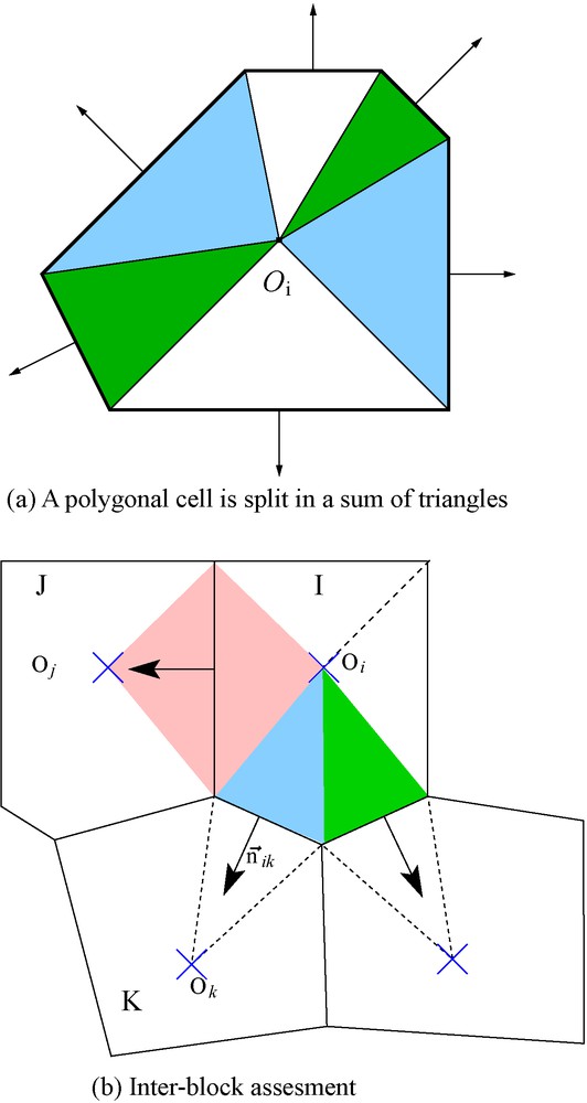
Renormalisation along the normal component. The geometry of the grid gives the local direction of the normal flow. For the intra-block formulation, the permeability is computed on each sub-triangle, with a final recomposition to obtain the equivalent permeability of the polygon. For the inter-block formulation, the equivalent permeability on each quadrangle (pair of adjacent triangles) is provided as is to the hydrodynamic model.
Fig. 2. Renormalisation suivant la composante normale. La géométrie du maillage fixe la direction du flux normal. Dans la version intra-bloc, on calcule les perméabilités de chaque triangle et on les recompose pour obtenir la perméabilité équivalente du bloc. Dans la version inter-bloc, la perméabilité équivalente de chaque « losange » est fournie directement au modèle.

Due to historical choices, the code Hytec uses only scalar components: indeed, in coupled reactive transport phenomena, the geochemistry often limits the effects on the transport of a possible anisotropy of the medium. Assuming isotropic conditions, the diagonal terms of the permeability tensor obtained by this method are combined following the direction of the normal flow, which is determined by the mesh geometry (by construction of the Voronï mesh). This inter-block permeability is used directly in the Hytec code: it corresponds to the mid-nodal permeability of finite differences. It is worth mentioning that the discretisation obtained by this method is finer than the finite volume partition of space for which the permeability would be uniform inside each polygon. To preserve the consistency with the finite volume formalism, a intra-block upscaling of the permeability can also be computed: each polygon can be divided in as many triangles as it has vertices (two adjacent vertices form the basis of the triangle, the centre of the polygon forms its summit); on these triangles, the simplified renormalisation yields a value of the equivalent permeability for a flow normal to the opposite side. The equivalent permeability are then composed to get the equivalent permeability of the polygon; an arithmetic composition has been chosen, weighted by the relative surface of each elementary triangle of the polygon.

For anisotropical cases, the reasoning is not so easy. Beyond the necessity to take the permeability tensor into account, it is no longer possible to use the simplification based on the normal component of the flow at each polygon interface, so that the renormalisation scheme has to be heavily modified.

In the following, all three modes of composition are tested: Matheron's mean, simplified renormalisation, renormalisation along the normal component of the flow. Each yields two values: an intra-block permeability (uniform inside each polygon), and an inter-block permeability (on the quadrilateral between the centre and adjacent side of each pair of adjacent polygons). For the simplified renormalisation, the (intra- or inter-block) scalar permeability is computed assessing a local direction of the flow parallel to the macroscopic head gradient, determined by the boundary conditions.

4 Design of the numerical experiments

The sensitivity study aims at discriminating between the influence of the spatial variability of the medium (represented by the geostatistical simulation on the fine grid) and the representation of this variability, which depends on the spatial discretisation for the finite volumes and the upscaling scheme. To this end, numerical experiments are carried out on geostatistical simulations of the permeability only; inter- or intra-block equivalent values are computed using all three upscaling methods, for several types of Hytec grids.

The domain of study is a permeameter: it consists in a rectangle, with a uniform inflow along a boundary, a uniform constant head condition along the opposite boundary, while the other two boundaries are impermeable (Fig. 3). The permeameter has been extended with two lines of cells just outside the control lines, for better control of the boundary conditions independently of the polygonal grid inside the permeameter. At the initial time, a perfect tracer A is at constant concentration 1 inside the permeameter; the incoming flow flushes the permeameter with a tracer B at concentration 1 (and no tracer A).

Fig. 3
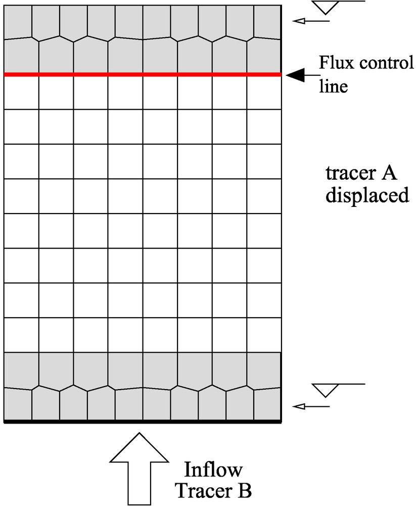
Boundary conditions for the numerical experiments.
Fig. 3. Conditions aux limites pour les expériences numériques.

In the bulk of the permeameter, the permeability K is assumed lognormally distributed, obtained from a (multi-) Gaussian random function Y:

K = M e^{σ \cdot Y - \frac{σ^{2}}{2}}

(3)

where M is the arithmetic mean, and σ² the logarithmic variance of the permeability. In this model, the spatial variability is characterised by the variogram γ of the random function Y. Once fixed the variogram model type (spherical, exponential), the set of parameters which fully describe the spatial model is limited to the range a (correlation length) and the standard deviation σ_{ln K} of the Napierian logarithm of the permeability. Due to the choice of boundary conditions, the flow is independent of the mean M of the permeability. We chose M = 10⁻³ m/s.

The results of the study are all presented adimensionally; e.g., the length of the field is fixed to L = 100 m: all the other parameters of the same dimension (range of the variogram, dispersivity,) are given relative to the unit L. For the hydrodynamics resolution, the time is expressed adimensionally, as a number of pore volumes injected (the total pore volume is equal to the surface of the permeameter in 2D multiplied by its mean porosity); we refer to this adimensional time also as “water renewal cycles”.

The observable chosen to describe the system is the cumulative flux of tracer through a control line at the outlet of the permeameter: tracer A, initially at concentration 1 inside the permeameter, is flushed out by the injection of fresh (A-free) water at the inlet. Throughout the study, we will show the cumulative flux of A through the outlet after an adimensional time 0.8 (i.e. after 80% of the pore volume has been renewed). This particular time is particularly interesting: later on, most of the initial tracer has been flushed, so that the cumulative fluxes are close to the initial total amount of A; for shorter amounts of time, the effects of the spatial variability are still limited to the neighbourhood of the inlet, and have low effects on the fluxes at the outlet.

Two series of numerical experiments were carried out. The first one is based on a 64 × 64 geostatistical simulation, which allows for a Hytec reference simulation, without preliminary upscaling. The upscaling techniques are then applied to build coarser Hytec grids: 16 × 16 and 8 × 8 rectangular grids. For both sizes, three classes of Hytec grids are investigated: regular rectangular, diamonds (actually 45°-tilted rectangles), and rectangular with diamond inclusion (Fig. 4); so that six coarse grids are investigated. For the second series of numerical experiments, 500 × 500 reference simulations have been attempted. However, the implicit geochemistry in Hytec (even for non-reactive tracer) leads to a degradation of the precision of the results for such fine grids; in our specific case, where precise comparisons of fluxes across a boundary are performed, the quality of the results were not sufficient to provide a definite reference. This point should be improved in further versions of Hytec.

Fig. 4
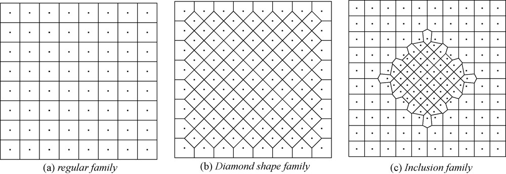
Grids for the second series of numerical experiments.
Fig. 4. Maillages de la deuxième série d’expériences.

For the first series of experiments, the 64 × 64 geostatistical simulations were performed by the discrete spectral method: the method is very CPU-effective, and offers the possibility to vary the range a at “constant random draw”, i.e. using the same realisation of random numbers. We can thus investigate the effect of the range without interference from the random variability between two draws [5]. For the second series of experiments, we chose the turning bands method; the code has not been adapted for this specific purpose, so that the 500 × 500 grid simulations for different ranges correspond to different random draws.

Three values were tested for the range of the spherical variogram of the Napierian logarithm of the permeability (Eq. (3)): a = 10, 30 and 50% of the length L of the permeameter. The five values chosen for the logarithmic standard deviation Ω_{ln K} are listed in Table 1. The other parameters were chosen as follows:

• high dispersivity: α = 0.1 × L;
• uniform porosity: ω = 0.3;
• effective diffusion coefficient: D_e=10⁻¹⁰ m²/s.

Variance (m²/s²)	10⁻⁴	5 × 10⁻⁵	10⁻⁵	5 × 10⁻⁶	10⁻⁶
σ _{ln K}	2.15	1.98	1.55	1.34	0.83

It is important to note the need for a careful control of the computation conditions on the precision of the result, for the chosen observable, particularly, the time step. Hytec determines an optimal time step, following several criteria (e.g., speed of convergence for the coupling); the maximum time step is bounded by the Courant–Friedrich–Levy stability criterion; however, a precise comparison between computations at different time discretisations revealed that the criterion was not stringent enough. We finally made all simulations with the same time step, based on the smaller time step obtained for the finer grid.

5 Experiments results

The transport computations were performed in an advective/dispersive framework, with a dispersion around 10³ times larger than diffusion. The dispersivity coefficient is quite high, around 0.1 times the length of the permeameter.

5.1 Simulations without numerical dispersion

The transport simulation using the centred scheme, without numerical dispersion, shows that the cumulative flux on a homogeneous medium are independent of the grid. In Fig. 5, the cumulative fluxes curves are strictly identical for the 64, 16 and 8 grids.

Fig. 5
Cumulative flux for the 64 × 64 reference grid; homogeneous permeability, range 0.1L and 0.5L and large standard deviation.
Fig. 5. Flux cumulés pour le maillage 64 × 64 de référence ; cas homogène et portées 0,1L et 0,5L avec écart-type élevé.

On the other hand, the upward scheme, with added numerical dispersion, produces a delay on the arrival of the tracer; the delay increases with the size of the polygons. The cumulative flux curves converge towards the theoretical limit (a proof that the code does not loose mass), but the time needed to converge towards the limit increases with coarser grids: indeed, for coarse grids, the numerical dispersion is larger, which clearly creates longer dispersion tails, and delays the complete flushing of the tracer.

In the following, results are given using the numerically dispersive scheme.

5.2 Upscaling between rectangular cells 64 × 64, 16 × 16, and 8 × 8

The parametric study is performed systematically using the same initial random realisation, and the several values for the geostatistical parameters: 5 values for σ, 3 for the range, 3 renormalisation methods, intra- or inter-block variation, fine initial grid and the two other grids.

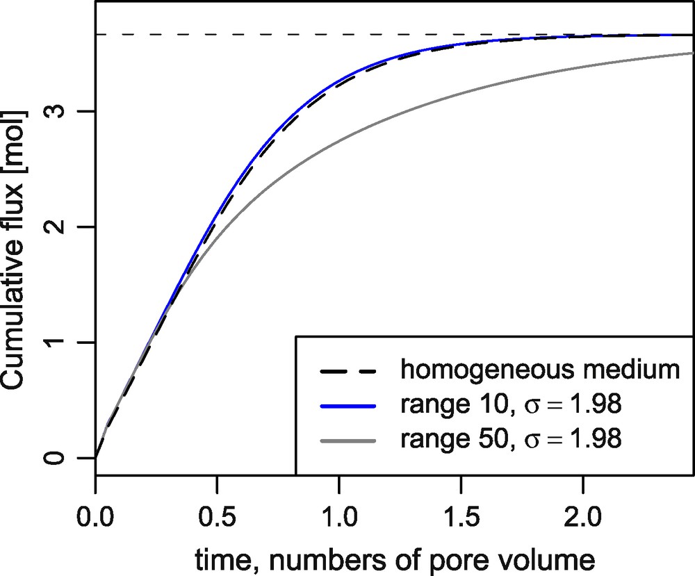
Fig. 6 shows the cumulative fluxes obtained on the reference simulation (64 × 64 grid), for media with range 0.1L and 0.5L. For a = 0.1L, the curves are superimposed for all variance values, and close to the uniform permeability reference. For a = 0.5L, the variance plays a major role: the cumulative fluxes diverge from the uniform permeability reference. A possible explanation is that longer range geostatistical simulations create spatially well-structured fluctuations in the flow velocity field; increasing variances accentuate the discrepancy between low and high permeability zones, so that the effect of preferential pathways increases.

Fig. 6
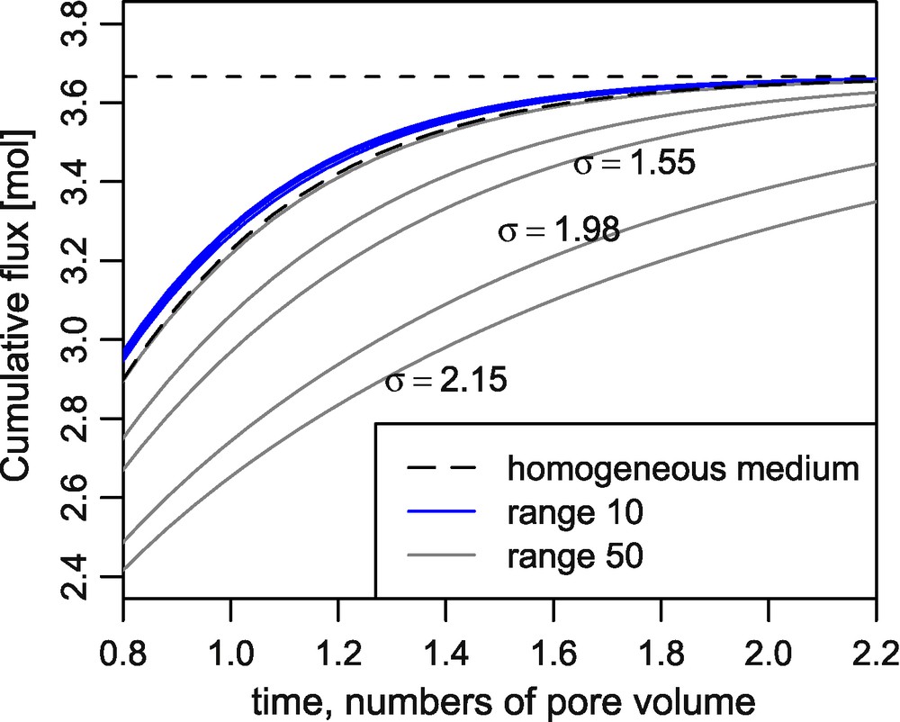
Cumulative flux for the 64 × 64 reference grid, compared to the homogeneous case. For the larger range, the logarithmic variance has a large impact; on the contrary, for the smaller range (in blue), the differences are very small.
Fig. 6. Flux cumulés sur maillage 64 × 64 de référence, comparés au cas homogène. Pour les grandes portées, la variance logarithmique a une grande influence ; au contraire, pour les faibles portées (en bleu), les écarts sont minimes.

The spatial variability of permeability systematically introduces a delay on the cumulative flux curves, compared to the homogeneous reference or small range or small variance simulations. In the short term, preferential pathways allow for a faster circulation of the tracer; however, in the longer term, slow circulation areas delay the complete flush of the tracer. The spatial variability has thus a dual effect on the system behaviour: the breakthrough of the tracer B is faster, but the complete leaching of the initial tracer A takes longer.

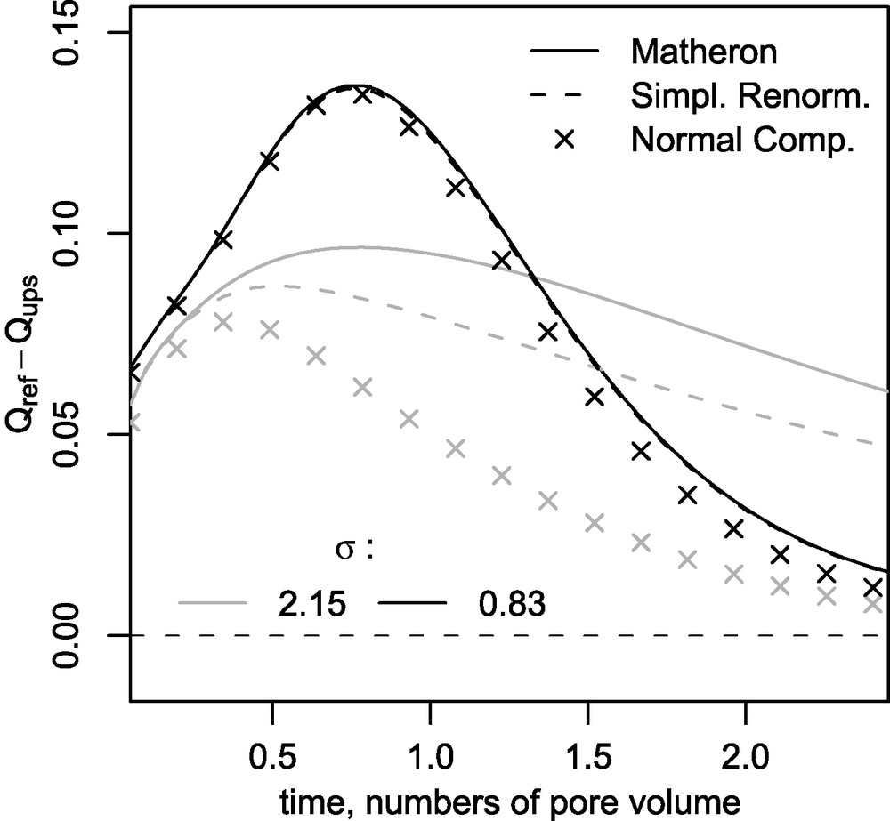
Let Q_ref(t) be the cumulative flux in the reference simulation, on the initial 64 × 64 grid, and Q_ups(t) the results after upscaling. Figs. 7–10 show the effect of the upscaling, as the difference Q_ups(t) − Q_ref(t). Indeed, in this case, the ratio Q_ups/Q_ref tends to decrease the difference between simulations results, so that it is not a good discriminating observable.

Fig. 7
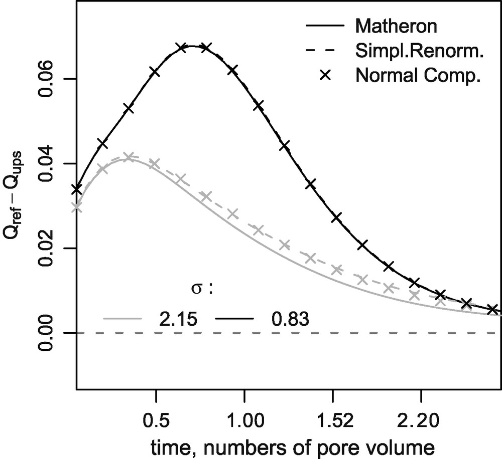
Difference of the cumulative flux relative to the reference simulation; 16 × 16 grid, inter-block formulation, range 0.3L.
Fig. 7. Écart du flux cumulé par rapport au calcul de référence ; grille 16 × 16, calcul inter-bloc, portée 0,3L.

Fig. 8
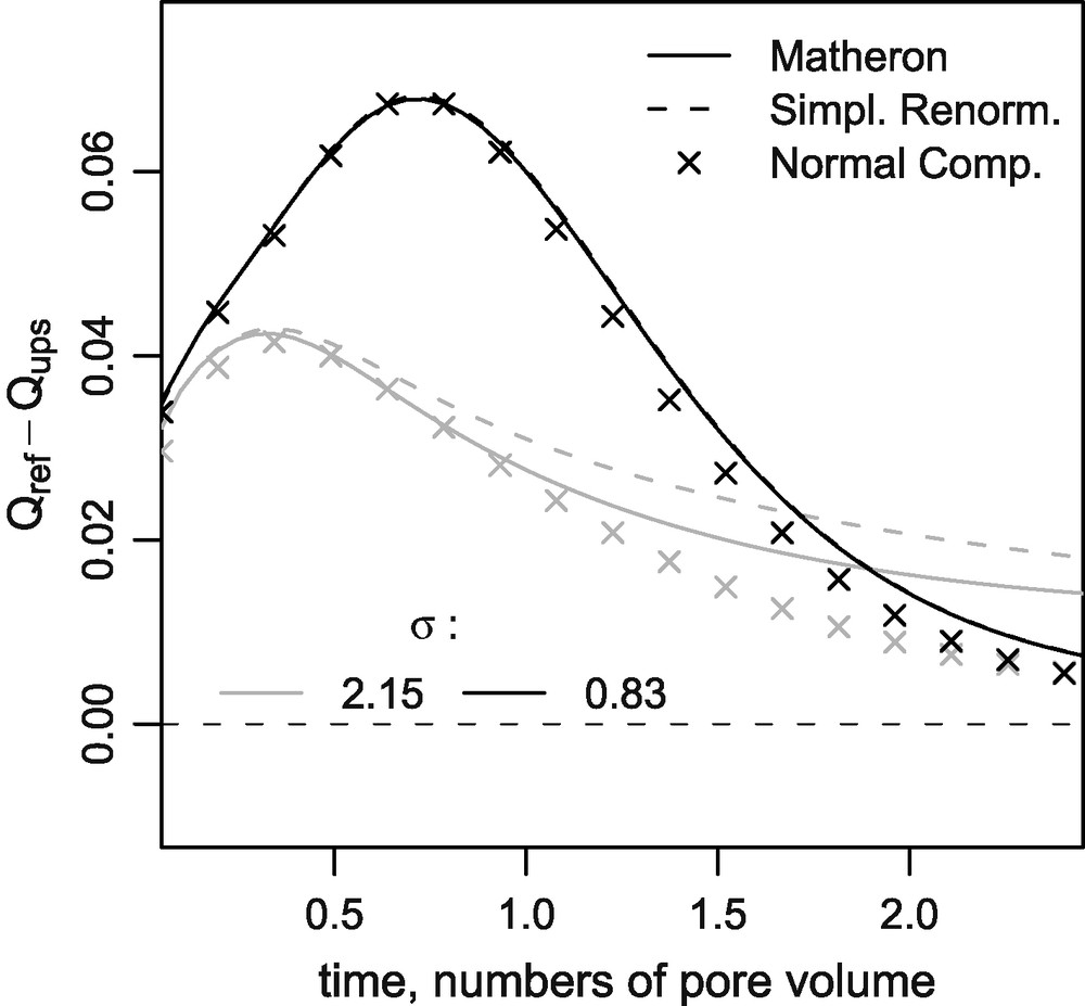
Difference of the cumulative flux relative to the reference simulation; 16 × 16 grid, inter-block formulation, range 0.5L.
Fig. 8. Écart du flux cumulé par rapport au calcul de référence ; grille 16 × 16, calcul inter-bloc, portée 0,5L.

Fig. 9
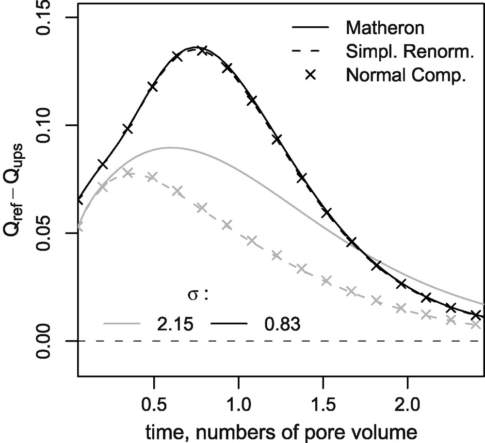
Difference of the cumulative flux relative to the reference simulation; 8 × 8 grid, inter-block formulation, range 0.3L.
Fig. 9. Écart du flux cumulé par rapport au calcul de référence ; grille 8 × 8, calcul inter-bloc, portée 0,3L.

Fig. 10
Difference of the cumulative flux relative to the reference simulation; 8 × 8 grid, inter-block formulation, range 0.5L.
Fig. 10. Écart du flux cumulé par rapport au calcul de référence ; grille 8 × 8, calcul inter-bloc, portée 0,5L.

The variance of the permeability discriminates between the curves. Unexpectedly, the maximum difference compared to the reference is obtained for small values of the variance. This can be explained by the transformations due to the upscaling, which modify the preferential pathways for a small variance. On the contrary, for larger values of σ, the preferential pathways are more pronounced, and resist to all the upscaling techniques. The differences between upscaling methods can be seen on the 16 × 16 grid (Figs. 7 and 8), and even more on the 8 × 8 grid (Figs. 9 and 10, with different scales than from that of the 16 × 16 grid figures).

Logically, the effect of the range on the upscaling is more related to its ratio to the mean size of the blocks. For the same range, the influence of the upscaling (of the hydrodynamic grid) increases with the block sizes (Figs. 7 and 9 on the one hand and Figs. 8 and 10 on the other hand). For a fixed hydrodynamic grid, the differences between the three upscaling methods increase with the range (Figs. 7 and 8 on the one hand and Figs. 9 and 10 on the other hand), and are greater when the variance increases.

It is not straightforward to set a hierarchy between the upscaling methods. For the inter-block method, the results of the normal component renormalisation are a little closer to the reference, compared to the simplified renormalisation. Matheron's mean is systematically less precise for the 8 × 8 grid, but better for the 16 × 16 grid.

5.3 Experiments on complex grids

A second series of numerical experiments was carried out, with higher relative influence of the upscaling, and with more complex spatial discretisations for the hydrodynamic resolution (Fig. 4). For that purpose, the geostatistical simulations were performed on a much finer grid 500 × 500. Two independent realisations for each range a = 0.1L, 0.3L and 0.5L were drawn using the turning bands method. It was thus possible to control the influence of the random draw, but as explained in section 4, a direct comparison of simulations with different range was no longer possible. A major difference, compared to the previous section, is the absence of a reference hydrodynamic simulation, as discussed in section 4.

The hydrodynamic simulation results for the different grids are presented via the cumulative flux of tracer A through the outlet relative to the flux for the same grid with uniform permeability. In the absence of reference, this smoothes the effects of the spatial discretisation.

The results are displayed in Figs. 11 and 12, respectively on the square 16 × 16 and 8 × 8 grid in the intra-block formulation. The different upscaling methods are represented by different line codes (dashes, dots,). The differences between the upscaling methods are visible only for the larger values of the range and the variance. The discrepancy also increases with larger block sizes. The results for the other types of grids (diamonds, and inclusion) give similar results.

Fig. 11
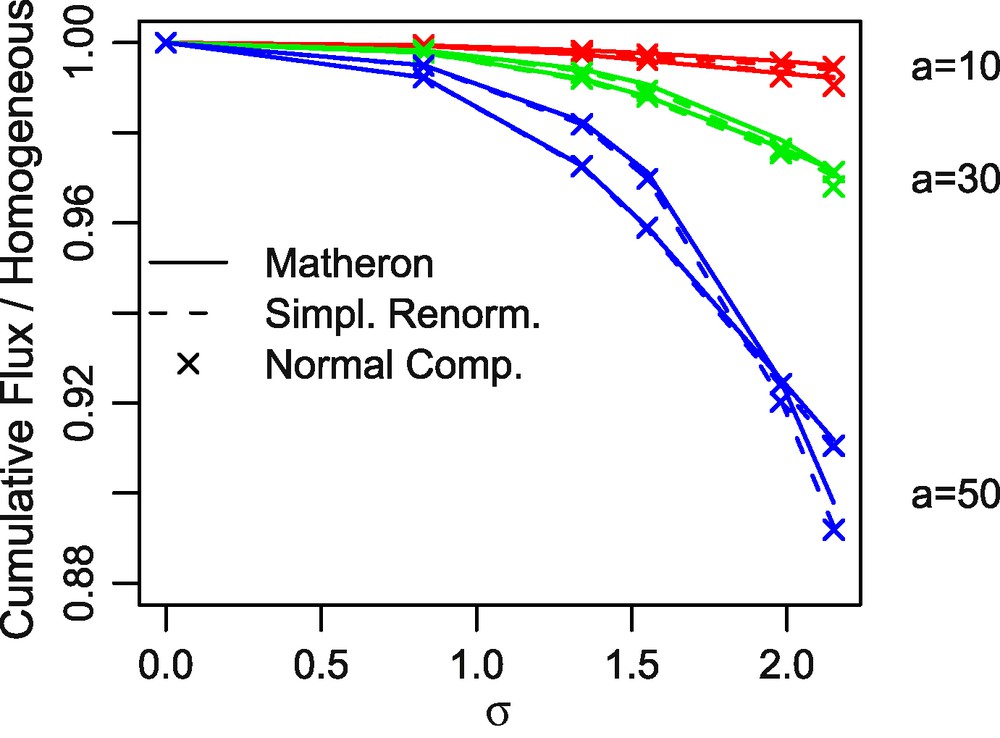
16 × 16 rectangular grid, intra-block formulation: ratio of the cumulative flux relative to the homogeneous case as a function of σ.
Fig. 11. Grille carrée 16, intra-bloc : rapport du flux cumulé à celui à perméabilité constante, en fonction de σ.

Fig. 12
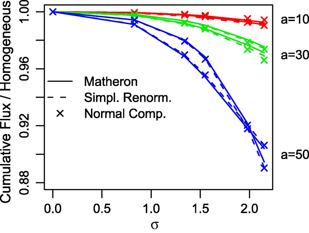
8 × 8 rectangular grid, intra-block formulation: ratio of the cumulative flux relative to the homogeneous case as a function of σ.
Fig. 12. Grille carrée 8, intra-bloc : rapport du flux cumulé à celui à perméabilité constante, en fonction de σ.

The impact of the random draw itself is far more important than the effect of the upscaling technique, particularly for range a = 0.5L. In this latter case, the field is not large enough to ensure the ergodicity of the realisation: the spatial mean can thus be different from its expectation.

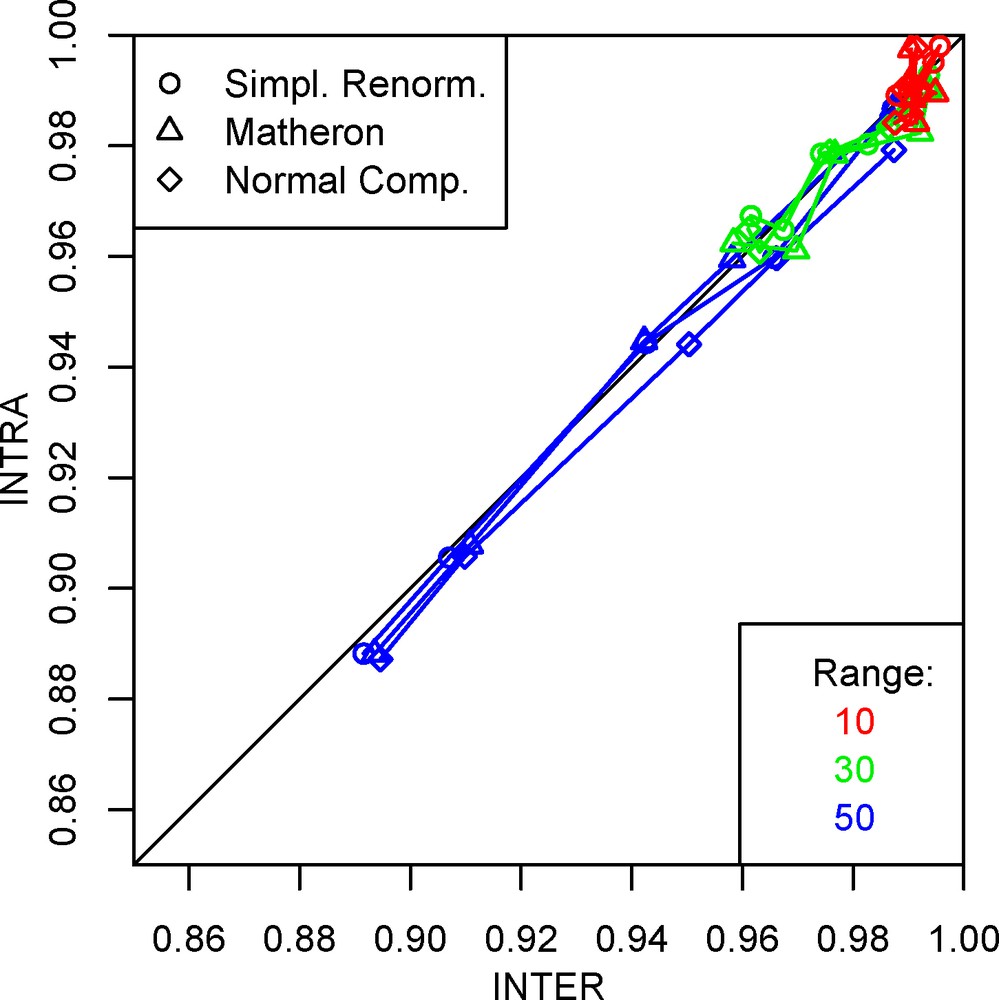
Owing to its limited influence (at least compared to the impact of the spatial variability itself), it is difficult to find systematic effects due to the upscaling techniques. Figs. 13 and 14 show a comparison for two 16 × 16 and 8 × 8 diamond-shape grids, in intra- and inter-block respectively. The inter-block formulation seems more robust relative to the mean size of the cells. This is understandable, since the implicit underlying grid for permeability is at least twice as fine for inter- than for intra-block. At any rate, the effects of upscaling towards coarser grids is more pronounced for the intra-block formulation.

Fig. 13
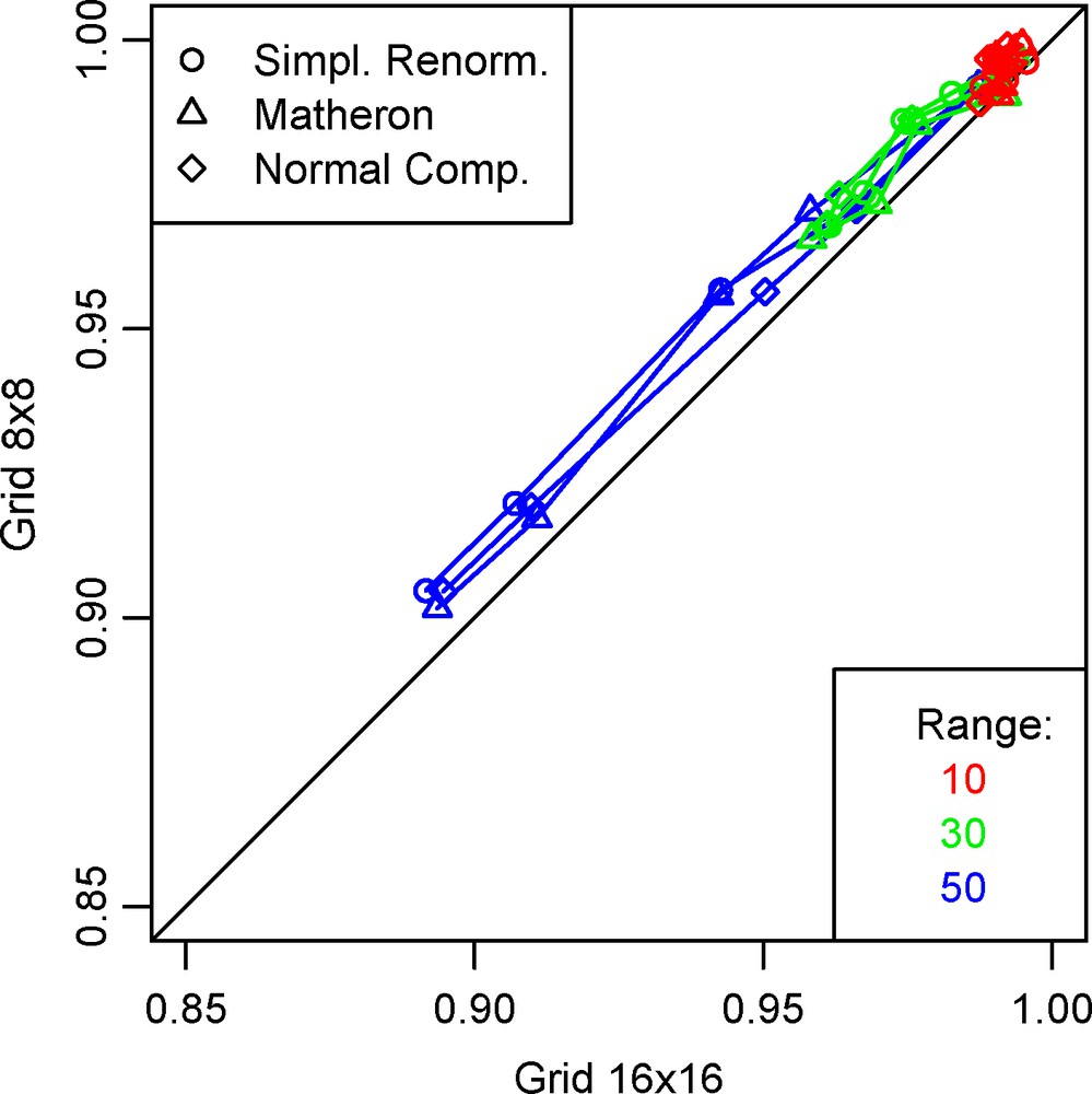
Scatter diagram of the cumulative flux relative to the uniform case, for several grids: diamond-shape size 8 and 16, intra-block formulation, all variances together.
Fig. 13. Nuage de corrélation entre les flux cumulés rapportés au cas à perméabilité constante, pour différents maillages : intra-bloc, grille losange 16 et 8, toutes variances confondues.

Fig. 14
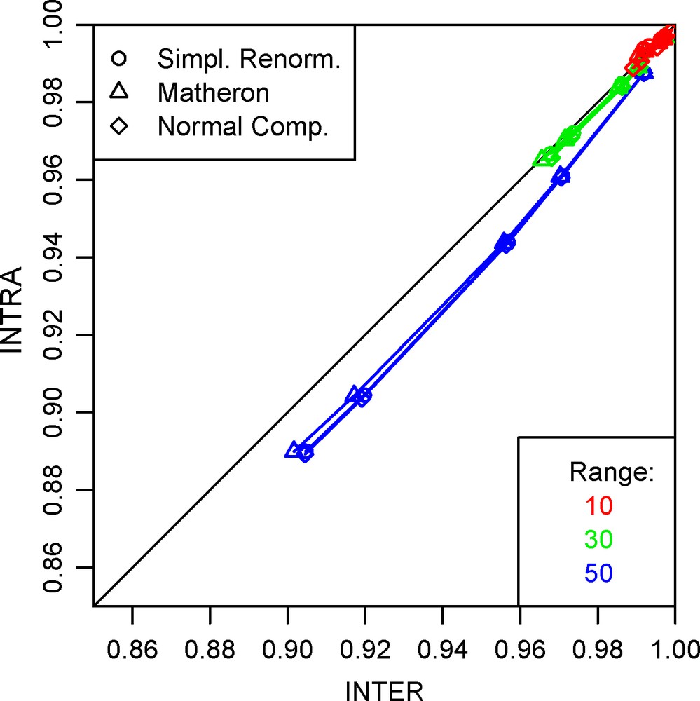
Scatter diagram of the cumulative flux relative to the uniform case, for several grids: diamond-shape size 8 and 16, inter-block formulation, all variances together.
Fig. 14. Nuage de corrélation entre les flux cumulés rapportés au cas à perméabilité constante, pour différents maillages : inter-bloc, grille losange 16 et 8, toutes variances confondues.

The cumulative fluxes obtained on a dense grid are generally lower than fluxes on a coarser grid (the points are below the first bisector on the scatter diagram), with the exception of the diamond-shape grids.

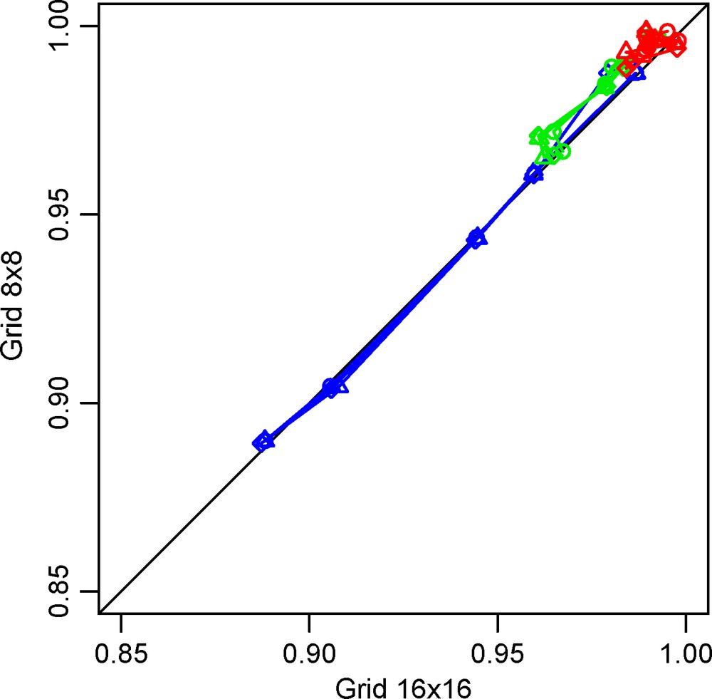
Figs. 15 and 16 (for the 16 × 16 and 8 × 8 diamond-shape grids, respectively) show a comparison between the inter- and intra-block formulations. It appears that the inter-block simulations yield systematically higher cumulative fluxes than the intra-block (the points are over the first bisector on the scatter diagram).

Fig. 15
Scatter diagram of the cumulative flux relative to the uniform case, for inter- and intra-block formulations; 16 × 16 diamond-shape grid, all variances together.
Fig. 15. Nuage de corrélation entre les flux cumulés rapportés au cas à perméabilité constante, pour le calcul inter-bloc et intra-bloc ; grille losange 16, toutes variances confondues.

Fig. 16
Scatter diagram of the cumulative flux relative to the uniform case, for inter- and intra-block formulations; 8 × 8 diamond-shape grid, all variances together.
Fig. 16. Nuage de corrélation entre les flux cumulés rapportés au cas à perméabilité constante, pour le calcul inter-bloc et intra-bloc ; grille losange 8, toutes variances confondues.

Finally, the simulations do not show systematic differences of behaviour between the three upscaling methods.

6 Conclusion

Several conclusions can be drawn from the comparison of the results on different simulated media and different hydrodynamic grids. The upscaling method itself has less influence on the cumulative flux of tracer at the outlet than the actual spatial discretisation (the hydrodynamic grid), or the effective spatial variability of the medium. The discrepancy between the three upscaling techniques for the inter-block permeability is even negligible, except for the larger values of the variance of the permeability and for the larger ranges. The three techniques do not display systematic effects (e.g., under-estimation). The geometry of the hydrodynamic grid should be carefully evaluated, and should be fully considered as one of the influential parameters for the observable.

Finally, the importance of the random draw has been displayed. Consequently, it could be worth devising a probabilistic quality criterion for the simulations; i.e., the best method should provide an unbiased estimation of the results distribution, at least in the mean or better in the mean and variance.

Acknowledgement

The study received a financial support by the European Union and University of Bologna. The authors are grateful for the positive reviews by B. Noetinger and R. Ababou who greatly helped improve the document.

Bibliographie

[1] J.E. Aarnes; V.L. Hauge; Y. Efendiev Coarsing of three-dimensional structured and unstructured grids for subsurface flow, Adv. Water Res., Volume 30 (2007), pp. 2177-2193

[2] R. Ababou Random porous media flow on large 3-D grids: numerics, performance and application to homogenizations, IMA, Mathematics and its applications: Environmental studies – Math., computational and statistical analysis, Vol. 79, Wheeler ed., Springer, New York, 1996, pp. 1-25

[3] V. Artus; B. Noetinger Up-scaling two-phases flow in heterogeneous reservoirs: current trends, Oil Gas Sci. Technol. Rev. IFP, Volume 59 (2004), pp. 185-195

[4] D. Bailly, R. Ababou, M. Quintard, Characterization and hydraulic behaviour of highly fissured geologic media (Karsts), IAHR-GW (Flow & transport in heterogeneous subsurface formations: theory, modelling & applications), Istanbul, Turkey, Proc. Internat. Symp., 2008.

[5] J.P. Chilès; P. Delfiner Geostatistics – modelling spatial uncertainty, Wiley & Sons, New York, 1999

[6] S.E. Gasda; M.A. Celia Upscaling relative permeabilities in a structured porous medium, Adv. Water Res., Volume 28 (2005), pp. 493-506

[7] C. He; L.J. Durlofsky Structured flow-based gridding and upscaling for modelling subsurface flow, Adv. Water Resour., Volume 29 (2006), pp. 1876-1892

[8] D.T. Hristopulos Renormalization group methods in subsurface hydrology: overview and applications in hydraulic conductivity upscaling, Adv. Water Res., Volume 26 (2003), pp. 1279-1308

[9] P. Jenny; S.H. Lee; H.A. Tchelepi Multi-scale finite volume method for elliptic problems in subsurface flow simulation, J. Comp. Phys., Volume 187 (2003), pp. 47-67

[10] M. Kfoury, Changement d’échelle séquentiel pour des milieux fracturés hétérogènes, Thèse, Institut de mécanique des fluides de Toulouse, 2004.

[11] M. Kfoury; R. Ababou; B. Noetinger; M. Quintard Upscaling fractured heterogeneous media: permeability and mass exchange coefficient, J. Appl. Mech. Trans. ASME, Volume 73 (2006), pp. 41-46

[12] M.J. King Recent Advances in upgridding, Oil Gas Sci. Technol. Rev. IFP, Volume 62 (2007), pp. 195-205

[13] V. Lagneau, R2D2 – Reactive transport and waterflow on an odd dimension 2 grid, Rapport technique, École des mines de Paris, 2007.

[14] J. van der Lee; L. De Windt; V. Lagneau; P. Goblet Presentation and application of the reactive transport code Hytec, Comput Methods Water Resour., Volume 1 (2002), pp. 599-606

[15] G. de Marsily Quantitative hydrogeology, groundwater hydrology for engineers, Academic Press, New York, 1986

[16] G. Matheron Eléments pour une théorie des milieux poreux, Masson, Paris, 1967

[17] A. Pouya Tenseurs de perméabilité équivalente d’un domaine hétérogène fini, C. R. Geoscience, Volume 337 (2005), pp. 581-588

[18] P. Renard, Modélisation des écoulements en milieux poreux hétérogènes. Calcul des perméabilités équivalentes, École des mines de Paris, Mem. Sci. Terre 32 (1997).

[19] P. Renard; G. de Marsily Calculating equivalent permeability: a review, Adv. Water Resour. Res., Volume 20 (1997), pp. 253-278

[20] P. Renard; G. Le Loc’h; E. Ledoux; G. de Marsily; R. Mackay A fast algorithm for the estimation of the equivalent hydraulic conductivity of heterogeneous porous media, Water Resour. Res., Volume 36 (2000), pp. 3567-3580

[21] F. Ubertosi; F. Delay; J. Bodin; G. Porel A new method for generating a pipe network to handle channelled flow in fractured rocks, C. R. Geoscience, Volume 339 (2007), pp. 682-691

Commentaires - Politique

Ces articles pourraient vous intéresser

The influence of spatial variability on 2D reactive transport simulations

Marco De Lucia; Vincent Lagneau; Chantal de Fouquet; ...

C. R. Géos (2011)

Statistical physics and applied geosciences: some results and perspectives

Benoît Noetinger

C. R. Phys (2020)

A hydrogeological acrostic: in honour of Ghislain de Marsily

Vazken Andréassian; Valérie Plagnes; Craig Simmons; ...

C. R. Géos (2023)