Miscible transfer of solute in different model fractures: From random to multiscale wall roughness

Harold Auradou; Alejandro Boschan; Ricardo Chertcoff; Maria-Veronica D’Angelo; Jean-Pierre Hulin; Irene Ippolito

doi:10.1016/j.crte.2009.03.003

Surfaces geosciences (Hydrology–Hydrogeology)

Miscible transfer of solute in different model fractures: From random to multiscale wall roughness
[Transport miscible de solutés dans différentes fractures modèles : influence de la rugosité aléatoire ou multiéchelles]

Présenté par : Written on invitation of the Editorial Board

Harold Auradou ^1,² ; Alejandro Boschan ^1,^2,³ ; Ricardo Chertcoff ³ ; Maria-Veronica D’Angelo ^1,^2,³ ; Jean-Pierre Hulin ^1,² ; Irene Ippolito ³

¹ Université Pierre-et-Marie-Curie Paris VI, 4, place Jussieu, 75252 Paris cedex 05, France
² Lab FAST (CNRS), université Paris-Sud, bâtiment 502, 91405 Orsay cedex, France
³ Grupo de Medios Porosos, Departamento de Fisica, Facultad de Ingenieria, Universidad de Buenos Aires, Paseo Colón 850, 1063 Buenos-Aires, Argentina

Comptes Rendus. Géoscience, Volume 342 (2010) no. 7-8, pp. 644-652.

Résumés

Anglais
Français

Miscible tracer dispersion measurements in transparent model fractures with different types of wall roughness are reported. The nature (Fickian or not) of dispersion is determined by studying variations of the mixing front as a function of the distance travelled but also as a function of the lateral scale over which the tracer concentration is averaged. The dominant hydrodynamic dispersion mechanisms (velocity profile in the gap, velocity variations in the fracture plane) are established by comparing measurements using Newtonian and shear thinning fluids. For small monodisperse rugosities, front spreading is diffusive with a dominant geometrical dispersion (dispersion coefficient D ∝ Pe or constant dispersivity l_d = D/U) at low Péclet numbers Pe; at higher Pe values, one has either l_d ∝ Pe (i.e. Taylor dispersion) for obstacles of height smaller than the gap, or l_d ∝ Pe^0.35 for obstacles bridging the gap. For a self-affine multiscale roughness like in actual rocks and a relative shear displacement $\vec{δ}$ of complementary walls, the aperture field is channelized in the direction perpendicular to $\vec{δ}$ . For a mean velocity $\vec{U}$ parallel to the channels, the global front geometry reflects the velocity contrast between them and is predicted from the aperture field. For $\vec{U}$ perpendicular to the channels, global front spreading is much reduced. Local spreading of the front thickness remains mostly controlled by Taylor dispersion except in the case of a very strong channelization parallel to $\vec{U}$ .

Nous présentons des mesures de dispersion de traceurs dans des modèles transparents de fractures présentant différents types de rugosités de parois. La nature de la dispersion (fickienne ou non) est déterminée à partir de l’évolution du front de mélange en fonction de la distance parcourue, mais aussi en faisant varier la distance transverse sur laquelle la concentration de traceur est moyennée. Les mécanismes de dispersion hydrodynamique dominants (profil de vitesse dans l’ouverture, variations de vitesse dans le plan de la fracture) sont identifiés en comparant des mesures utilisant des fluides newtoniens et rhéofluidifiants. Pour des parois avec des rugosités monodisperses de petite taille, l’étalement du front est diffusif et dominé par la dispersion géométrique aux faibles nombres de Péclet Pe (coefficient de dispersion D ∝ Pe d’où une dispersivité l_d = D/U constante); aux valeurs de Pe plus élevées, on a soit l_d ∝ Pe (i.e. dispersion de Taylor), pour des obstacles de hauteur plus faible que l’ouverture ou l_d ∝ Pe^0.35, lorsque la hauteur des obstacles est identique à l’intervalle entre les parois. Pour une rugosité autoaffine multiéchelle semblable à celle des roches naturelles et dans le cas de parois de géométries complémentaires, avec un déplacement relatif latéral $\vec{δ}$ , le champ d’ouverture est chenalisé dans la direction perpendiculaire à $\vec{δ}$ . Pour une vitesse moyenne $\vec{U}$ parallèle aux chenaux, la géométrie globale du front reflète les contrastes de vitesses entre ceux-ci et peut être prédite à partir du champ d’ouverture. Lorsque $\vec{U}$ est perpendiculaire aux chenaux, l’étalement global du front est fortement réduit. Quelle que soit la direction du décalage, l’étalement local du front reste contrôlé par la dispersion de Taylor; cependant, lorsque le décalage est trop fort et l’écoulement trop chenalisé, le transfert entre chenaux modifie ce comportement.

Métadonnées

Reçu le : 2008-11-07
Accepté le : 2009-03-17
Publié le : 2009-07-09

DOI : 10.1016/j.crte.2009.03.003

Keywords: Fractures, Roughness, Dispersion, Multiscale, Self-affine, Shear-thinning
Mot clés : Fractures, Rugosité, Dispersion, Multiéchelle, Auto-affine, Rhéofluidifiant

Affiliations des auteurs :

Harold Auradou ^{1, 2} ; Alejandro Boschan ^{1, 2, 3} ; Ricardo Chertcoff ³ ; Maria-Veronica D’Angelo ^{1, 2, 3} ; Jean-Pierre Hulin ^{1, 2} ; Irene Ippolito ³

@article{CRGEOS_2010__342_7-8_644_0,
     author = {Harold Auradou and Alejandro Boschan and Ricardo Chertcoff and Maria-Veronica D{\textquoteright}Angelo and Jean-Pierre Hulin and Irene Ippolito},
     title = {Miscible transfer of solute in different model fractures: {From} random to multiscale wall roughness},
     journal = {Comptes Rendus. G\'eoscience},
     pages = {644--652},
     publisher = {Elsevier},
     volume = {342},
     number = {7-8},
     year = {2010},
     doi = {10.1016/j.crte.2009.03.003},
     language = {en},
}

TY  - JOUR
AU  - Harold Auradou
AU  - Alejandro Boschan
AU  - Ricardo Chertcoff
AU  - Maria-Veronica D’Angelo
AU  - Jean-Pierre Hulin
AU  - Irene Ippolito
TI  - Miscible transfer of solute in different model fractures: From random to multiscale wall roughness
JO  - Comptes Rendus. Géoscience
PY  - 2010
SP  - 644
EP  - 652
VL  - 342
IS  - 7-8
PB  - Elsevier
DO  - 10.1016/j.crte.2009.03.003
LA  - en
ID  - CRGEOS_2010__342_7-8_644_0
ER  -

%0 Journal Article
%A Harold Auradou
%A Alejandro Boschan
%A Ricardo Chertcoff
%A Maria-Veronica D’Angelo
%A Jean-Pierre Hulin
%A Irene Ippolito
%T Miscible transfer of solute in different model fractures: From random to multiscale wall roughness
%J Comptes Rendus. Géoscience
%D 2010
%P 644-652
%V 342
%N 7-8
%I Elsevier
%R 10.1016/j.crte.2009.03.003
%G en
%F CRGEOS_2010__342_7-8_644_0

Harold Auradou; Alejandro Boschan; Ricardo Chertcoff; Maria-Veronica D’Angelo; Jean-Pierre Hulin; Irene Ippolito. Miscible transfer of solute in different model fractures: From random to multiscale wall roughness. Comptes Rendus. Géoscience, Volume 342 (2010) no. 7-8, pp. 644-652. doi : 10.1016/j.crte.2009.03.003. https://comptes-rendus.academie-sciences.fr/geoscience/articles/10.1016/j.crte.2009.03.003/

Version originale du texte intégral

1 Introduction

The geothermal reservoir of Soultz-sous-Forêts, like most geological systems, contains structures of various sizes along which flow occurs; three main types of structures were identified: individual fractures, fracture clusters and major faults (Genter et al., 1997). In order to understand these flow systems and help with managerial decisions, large scale numerical models incorporating such heterogeneities have been developed. Yet, when the transport of solutes is involved, the choice of a dispersion law (possibly scale dependent) valid at the scale of an individual fracture remains an open issue (NAS Committee, 1996).

At this scale, tracer dispersion results from the combined action of the complex velocity field (varying both in the gap of the fracture and in its plane) and of mixing by molecular diffusion. The latter allows the tracers to move from one streamline to another and homogenizes the spatial distribution of the tracers. In the classical approach, tracer particles are assumed to perform a random walk superimposed over a drift velocity. The latter is the average of the fluid velocity over an appropriate volume (the representative elementary volume or REV) while smaller scale variations induce tracer spreading. At the REV scale, the average $\bar{C} (x, t)$ of the tracer concentration over a section of the medium normal to the mean displacement satisfies the convection-diffusion equation (Auradou et al., 2005):

\frac{\partial \bar{C} (x, t)}{\partial t} = U \frac{\partial \bar{C} (x, t)}{\partial x} + D \frac{\partial^{2} \bar{C} (x, t)}{\partial x^{2}}

(1)

where D is the longitudinal dispersion coefficient and U the mean velocity of the fluid (parallel to x). The value of D (or equivalently of the dispersivity l_d = D/U) is independent of both time and the distance travelled: it is determined by the combined contributions of molecular diffusion and advection. The relative order of magnitude of these two effects is characterized by the Péclet number: Pe = Ua/D_m (D_m is the molecular diffusion coefficient; a is a characteristic length of the medium: here the mean fracture aperture).

Several experimental studies of breakthrough curves of solutes in natural fractures reported in the literature (Keller et al., 1999; Lee et al., 2003; Neretnieks et al., 1982; Park et al., 1997) measured dispersion coefficients increasing linearly with the mean flow U (or with Pe). Moreover, the value of the dispersivity l_d = D/U observed agreed with the predictions of a perturbation analysis (Gelhar, 1986). These results suggested that dispersion is controlled (as in 3D porous media (Bear, 1972)) by spreading due to velocity variations associated to the geometry of the void structure. This determines the correlation length of the velocity field, leading to the so-called geometrical dispersion regime. However, flow in fractures is known to be frequently concentrated in long channels of high hydraulic conductance (Brown et al., 1998; NAS Committee, 1996; Tsang and Tsang, 1989). The velocity remains then correlated over distances which may be too large for establishing a Fickian dispersion regime. These previous experiments were all performed for a fixed path length: however, in order to test the validity of the Fickian description, one must measure the variation of the width of the mixing front with time t and check whether it increases, as expected, as t^1/2.

Another key factor is dispersion resulting from the flow profile in the gap of the fracture: the variation of the velocity between the walls (where it cancels out) and the middle of the gap (where it has a maximal value) stretches the solute front. This creates a concentration gradient across the gap which is balanced by transverse molecular diffusion. The decorrelation of the velocity of the solute is then determined by the characteristic time for the diffusion of solute particles across the gap. This differs from the geometrical regime in which the decorrelation is determined by the geometrical structure of the fracture. Then, the longitudinal dispersivity scales like l_d ∝ Pe in this so-called Taylor dispersion (instead of l_d ∼ cst for geometrical dispersion).

In fractures, both dispersion regimes are expected to coexist (Detwiler et al., 2000; Ippolito et al., 1993; Roux et al., 1998): at low Péclet numbers (but large enough to neglect pure molecular diffusion), dispersion is controlled by the disordered geometry, while, at higher ones, Taylor dispersion becomes the leading dispersion mechanism. However, the critical Péclet number characterizing the transition still has to be determined. Also, the robustness of this model, when contact points between the fracture walls are present, must be tested.

We discuss in this article dispersion experiments dealing with these issues and carried out in transparent fractures with various degrees of heterogeneities. The geometries of the void space and the roughness of the walls of these models are described in Section 2.1. They range from a random wall roughness with a correlation length of the order of the aperture to a multiscale rough wall geometry similar to that observed in the field (Sausse, 2002); this latter case often leads to a strong flow channelization (Tsang and Tsang, 1989). In the present models, a relative shear displacement $\vec{δ}$ of complementary matching rough walls is introduced: high aperture channels oriented normal to the displacement and spanning over the fracture are then created leading to an anisotrope aperture field (Auradou et al., 2005; Gentier et al., 1997). This phenomenon increases with the magnitude of $\vec{δ}$ and becomes noticeable as soon as δ is of the order of the mean aperture (Matsuki et al., 2006). The influence of the contact area between the fracture walls was also investigated by performing flow experiments in a transparent model fracture with an array of contact points.

In order to address these various issues, dispersion has been studied as a function of:

• the distance traveled by the tracer;
• the lateral scale of observation in the fracture plane over which the concentration is averaged. This scale ranges from a (meso)microscopic scale (i.e. the typical fracture aperture) up to the fracture width;
• the fluid rheology in order to determine, without ambiguity, the main mechanisms controlling the dispersion: i.e. velocity profile in the fracture gap or velocity fluctuations in the fracture plane.

This contrasts with previous measurements realized at the outlet of the samples and in which the development of the mixing region and its spatial structure cannot be investigated.

2 Experimental setup and procedure

2.1 Experimental models and injection set-up

All models are transparent and placed vertically with their open sides horizontal. The upper side is fitted with a leak-tight adapter allowing one to suck the fluid at a constant flow rate. The lower open side can be dipped into a bath containing the liquid. When the pump is switched off, the bath can be lowered before changing the fluid inside it. This allows one to obtain a flat initial front between the fluids (See Figure 1 in ref (Boschan et al., 2007)).

The models are illuminated from the back by a light panel and images are acquired using a high resolution camera. The pixel size is around 0.2 mm, i.e. lower than the typical fracture aperture. About 100 images of the distribution of the light intensity I(x,y,t) transmitted through the fracture are recorded at constant intervals during the fluid displacement using a digital camera with a high dynamic range. Reference images with the fracture saturated with the clear and dyed fluids (dye concentration c₀) are also recorded before the experiments and after the full saturation by the displacing fluid. A calibration curve obtained independently through separate measurements is then used to map the local relative dye concentration 0 ≤ c(x,y,t)/c₀ ≤ 1 (in the following, c₀ is omitted and c(x,y,t) refers directly to the normalized dye concentration). The two fluids are of equal density: this is verified by performing twice the experiments at each flow rate value with the dyed fluid either displacing or displaced by the clear fluid. Comparing the results allows one to detect possible instabilities induced by residual density differences (the corresponding experiments are discarded). The two fluids are, of course, miscible and have the same viscosity.

2.2 Fluids preparation and characterization

The solutions used in the present work are either a Newtonian water-glycerol mixture or shear-thinning water-polymer (scleroglucan) solutions with a 500 or 1000 ppm polymer concentration. In all cases, the injected and displaced fluids have identical rheological properties. The Newtonian solution contains 10% in weight of glycerol and has a viscosity equal to 1.3 × 10⁻³ Pa s at 20 °C. The preparation and characteristics of the shear-thinning solutions are the same as those reported in (Boschan et al., 2007). The variation of the viscosity μ with the shear rate $\dot{γ}$ is well fitted by the Carreau function:

μ = \frac{1}{{(1 + {(\dot{γ} / {\dot{γ}}_{0})}^{2})}^{(1 - n) / 2}} (μ_{0} - μ_{\infty}) + μ_{\infty} .

(2)

The values of the rheological parameters characterizing the fluids are listed in Table 1. For the non Newtonian fluids and at low shear rates

\dot{γ} ≲ {\dot{γ}}_{0}

, the viscosity is constant, as for a Newtonian fluid with

μ ≃ μ_{0}

(Newtonian plateau regime). At higher shear rates

\dot{γ} {\dot{γ}}_{0}

, the viscosity follows a power law:

μ \propto {\dot{γ}}^{(n - 1)}

. Practically, μ_∞ is taken equal to 1 mPa s, i.e. the viscosity of water (the solvent): this limiting value would indeed only be reached at shear rates above the experimental range.

Fluids	n	${\dot{γ}}_{0} s^{- 1}$	μ₀ mPa.s
W-Glycerol	1	–	10
500 ppm	0.38 ± 0.04	0.077 ± 0.018	410 ± 33
1000 ppm	0.26 ± 0.02	0.026 ± 0.004	4500 ± 340

The two main dispersion mechanisms, i.e., Taylor dispersion (l_d ∝ Pe) and geometrical dispersion (l_d ∼ cst) are affected in opposite directions when a Newtonian fluid is replaced by a shear thinning solution. More precisely, the velocity contrasts between different flow paths are enhanced for a shear thinning fluid, resulting in an increase of the geometrical dispersion (without modifying the relation l_d ∼ cst). By contrast, the velocity profiles in the gap become flatter: this reduces therefore Taylor dispersion, but still with l_d ∝ Pe. Varying the fluid rheology modifies the relative influence of the two main dispersion mechanisms in opposite ways: the dominant one can therefore be identified unambiguously for each fracture geometry and flow rate.

3 Experimental results

3.1 Fracture model 1

In this model, flow takes place in the free space between a flat plate and a second one with protuberant obstacles. The latter perturb the flow velocity field: the local mean fluid velocity (averaged over the gap) is greater between the obstacles, where the aperture is largest than at their top, where it is minimal. These mean velocity variations in the fracture plane result in geometrical tracer spreading. As for the velocity profile in the fracture gap, it induces Taylor-like dispersion. The variation of the dispersivity l_d = D/U as a function of Pe confirms that it is the sum of the two contributions discussed above with:

\frac{l_{d}}{a} = α_{G} + α_{T} P e,

(3)

where α_TPe corresponds to Taylor dispersion and α_G to geometrical dispersion. Longitudinal molecular diffusion introduces an additional term α_D/Pe in which α_D < 1 reflects the tortuosity of the medium: this term is, however, omitted here because it would only become significant compared to α_G at Pe values below the experimental range. For a fracture with two flat parallel plates and a Newtonian fluid, one has: α_G = 0 and α_T = 1/210; also, one has α_G ≠ 0 only for fractures with rough walls. Moreover, if the correlation length of the velocity field is small compared to the fracture size and if the ratio ɛ of the amplitude of the velocity fluctuations to the mean velocity U is small, then the perturbation theory predicts that α_G ∝ ɛ² (a complete expression of α_G is given by Eq. (3) of (Boschan et al., 2008)).

Experimental dispersivity variations as a function of Pe are plotted in Fig. 1 for the three fluids. These data sets are well adjusted (see lines in Fig. 1) by functions of the type shown in Eq. (3): the dispersivity increases at first slowly with Pe above $P e ≃ 20$ from a nearly constant plateau value before displaying a linear variation at higher velocities. The plateau value corresponds to α_G in Eq. (3) and increases with the polymer concentration. It can be shown that the amplitude of the velocity fluctuations is larger for shear thinning fluids: for a power law dependence of the viscosity on the shear rate $(μ \propto {\dot{γ}}^{(n - 1)})$ , the parameter ɛ would increase theoretically by a factor (1 + 1/n)/2 compared to a Newtonian fluid. The velocity fluctuations (and, as a result, the dispersivity) increase therefore when n decreases, i.e, when the shear thinning character of the fluids is stronger. Unlike α_G, the parameter α_T for shear-thinning fluids is lower than the Newtonian value 1/210 (Boschan et al., 2008).

Fig. 1
Variation of the experimental dispersivity l_d as a function of the Péclet number in model 1. (, ): water-glycerol solution; (, ): 1000 ppm, (, ): 500 ppm polymer solutions. l_d is determined from variations of the local concentration (filled symbols) or of its average over the model width (open symbols). Solid, dotted and dashed lines: fits of the data for each solution (in the above order) with Eq. (3).
Variation de la valeur expérimentale de la dispersivité l_d en fonction du nombre de Péclet Pe dans le modèle 1. (, ) : solution eau-glycérol; solutions de polymère de concentrations: (, ) 1000 ppm et (, ) 500 ppm. l_d est déterminée à partir des variations de la concentration locale (symboles pleins) ou de sa moyenne sur la largeur du modèle (symboles vides). Lignes continues, pointillées, tirets: ajustement des données par l’Éq. (3) pour chaque solution (dans l’ordre précédent).

The values represented in Fig. 1 by filled symbols were obtained by fitting variations with time of the local concentration on each individual pixel by solutions of Eq. (1); this provides local values of both the dispersion coefficient D(x,y) and the transit time. The values of D(x,y) at points far enough from the inlet so that dispersion has reached a stationary regime are then averaged over x and y. A similar analysis was performed on the average of the local concentrations over the fracture width and its results are displayed by empty symbols in Fig. 1: they almost fall on the filled symbols demonstrating the lack of large scale concentration heterogeneities in the mixing front.

3.2 Fracture model 2

In this model, the obstacles extend over the full gap height and mimic gouge particles created by the failure of the rock and evenly distributed in the fracture (Section 2.1). The model is then a plane array of channels of random width: it can be considered as a 2D porous medium in which the pores correspond to the junctions between the channels. We show now that mixing at these junctions has a crucial influence on dispersion.

Fig. 2 displays variations of the dispersivity with the Péclet number deduced from time variations of the local concentration at the pore scale (filled symbols) and of its average over the fracture width (open symbols); it is seen that the values of l_d obtained in both cases are similar so that, in the following, only global measurements will be discussed.

Fig. 2
Variation of the dispersivity l_d (mm) with the Péclet number for experiments with water-polymer solutions: (),(): 500 ppm concentration - (), () 1000 ppm. Open (resp. filled) symbols: averaging interval: 35 (resp. 0.4) mesh sizes. Dashed lines: Mean dispersivity values for the geometrical dispersion regime. Dotted line: power law fit of the variation for Pe > 10 (exponent 0.35 ± 0.03).
Variation de la dispersivité l_d (mm) avec le nombre de Péclet Pe pour des expériences avec des solutions eau-polymère de concentrations: (),() 500 ppm et (), () 1000 ppm. Symboles ouverts (resp. pleins) : intervalle de moyennage : 35 (resp. 0,4) tailles de maille. Tirets : valeurs de dispersivité moyennes pour le régime de dispersion géométrique. Pointillés: ajustement par une loi de puissance de la variation pour Pe > 10 (exposant 0,35 ± 0,03).

For Pe < 10, l_d = D/U, is nearly constant (i.e. D ∝ Pe), suggesting dominantly geometrical dispersion. As discussed in Sec. 3.1, the value of l_d in this regime should depend strongly on the rheology of the solution: more precisely, it should increase with the polymer concentration as indeed observed here (like for model 1).

For Pe > 10, a second dispersion regime is observed, in which l_d increases with Pe. Furthermore, the linear trend observed in a log-log coordinate shows that l_d follows a power law of Pe (more precisely, l_d ∝ Pe^0.35 for Pe > 10). This result is in agreement with numerical simulations by Bruderer and Bernabe (Auradou et al., 2008) and differs from the Taylor dispersion regime l_d ∝ Pe observed in model 1 at high Pe values. This difference is explained by the influence of the pore junctions. At low flow velocities (typically Pe < 10), tracer particles can explore effectively the local flow field by molecular diffusion during their transit time through a given junction: this distributes evenly the tracer concentration inside it which represents a perfect mixing condition. Then, the tracer concentration is equal in all outgoing paths and the probability to follow one of them is proportional to the corresponding flow rate (Adler and Thovert, 1999; Park et al., 2001). Therefore, in this regime, dispersion is controlled by the disordered geometry of the array of channels.

At higher Pe values (typ. Pe > 10), mixing at the junctions is no more perfect and the tracer concentration in slower channels (like those transverse to the mean flow) is lower compared to the perfect mixing situation. The dispersion characteristic becomes more similar to the case of capillary tubes (representing the fast flow channels) oriented along the flow direction. In this case, one would observe Taylor dispersion with l_d ∝ Pe but the influence of flow redistribution at the junctions is quite large: this leads to a variation of l_d as Pe^0.35 intermediate between those observed in the geometrical and Taylor regimes. The origin of power law variations of l_d with Pe is also discussed in detail in (Bijeljic and Blunt, 2006).

3.3 Fracture model 3

Like in model 1, the walls of this fracture do not have any contact point but, in contrast with it, the rugosities of the wall have been selected to reproduce the multi-scale roughness of most natural fractures (Section 2.1).

Such fractures are known to display high aperture channels perpendicular to the relative shear displacement $\vec{δ}$ of the walls; they are characterized by an anisotropic permeability field with a larger permeability in the direction parallel to the channels. While most studies of these systems have dealt with their permeability, little is known about the influence of such a structure on tracer dispersion.

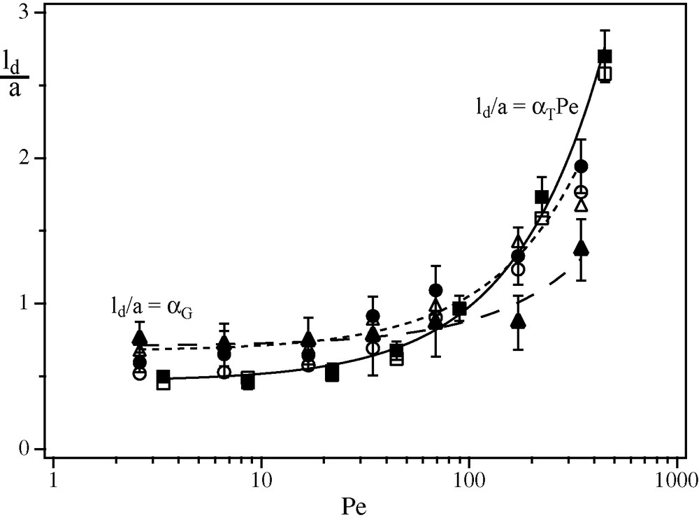
In model 3, flow is parallel to $\vec{δ}$ (i.e. normal to the channels): in this case $(\vec{δ} | | \vec{U})$ , the concentration variation curves are well adjusted by the solution of the convection-dispersion equation (1). This can be seen in Fig. 3 (+ symbols) both for the variations of the local concentration C(x,y,t) at a point (x,y) (inset) and for its average $\bar{C} (x, t)$ in the y direction across the model. Moreover, the dispersivities determined from these curves were found to become constant after a long enough path inside the fracture. As in models 1 and 2, the dispersion process is therefore Fickian. Fig. 4 displays variations of both the local and global dispersivities with Pe for the two polymer solutions. Theoretical Taylor dispersivities for a fracture of same mean aperture with plane smooth walls and for the different fluid rheologies are also plotted in Fig. 4 as dashed and dotted lines (differences between these curves reflect the effect of the velocity profile in the gap).

Fig. 3
Compared time variations of the average $\bar{C} (x, t)$ of relative concentration across the width of models 3 and 4 at a distance x = 285 mm from the inlet for dispersion experiments at a same Péclet number Pe = 285. Insert: time variation of the local relative concentration C(x,y,t) at a point (x,y) for the same distance x as for $\bar{C} (x, t)$ . Experimental data points: (+) for model 3 and (×) for model 4. Solid lines: fit of the corresponding data with the solution of Eq. (1). $\bar{t} (x, y)$ and $\bar{t} (x) = mean transit time determined by the fits$ .
Comparaison des variations temporelles de la moyenne $\bar{C} (x, t)$ sur la largeur des modèles 3 et 4, à une distance x = 285 mm de la face d’entrée, pour des expériences de dispersion à un même nombre de Péclet Pe = 285. Insert : variation temporelle de la concentration C(x,y,t) en un point (x,y) correspondant à la même distance x que $\bar{C} (x, t)$ . Données expérimentales : modèle 3 (+), modèle 4 (×). Lignes continues: ajustement des données correspondantes par une solution de l’Éq. (1). $\bar{t} (x, y)$ et $\bar{t} (x)$ : temps de transit moyens déterminés par les ajustements.

Fig. 4
Variation of the normalized dispersivity l_d/a as a function of Pe for model 3 and two different polymer concentrations. (, ): global dispersivities determined from concentrations averaged over the fracture width. (, ): local dispersivities determined from concentration variations on individual pixels. Lines: Taylor dispersion for plane parallel walls with the same mean gap as for model 3. (, ), dotted line: 1000 ppm polymer solution; (, ), dashed line: 500 ppm polymer solution; continuous line: Newtonian solution. Insert: variation of the ratio of the local and global dispersivities as a function of the Péclet number. (): 500 ppm solution. (): 1000 ppm solution.
Variation de la dispersivité normalisée l_d/a en fonction de Pe pour deux concentrations en polymère différentes dans le modèle 3. (, ): dispersivités globales déterminées à partir de la moyenne de la concentration sur la largeur de la fracture. (, ) : dispersivités locales déterminées à partir des variations de concentration sur des pixels isolés. Lignes : dispersion de Taylor entre des parois planes et parallèles avec le même intervalle que pour le modèle 3. (, ), ligne pointillée: solution de polymère de concentration 1000 ppm ; (, ), tirets : solution de concentration 500 ppm; ligne continue : solution newtonienne. Insert : variation du rapport des dispersivités locale et globale en fonction du nombre de Péclet. () : solution de concentration 500 ppm. () : solution de concentration 1000 ppm.

For Pe > 12, the local dispersivity increases with Pe in qualitative agreement with theoretical expectations (l_d ∝ Pe) and is also lower for the strongly shear-thinning 1000 ppm solution (open symbols). For both solutions l_d is larger than predicted, particularly for the 500 ppm solution for which it is close to the Newtonian value. This may be due to the vicinity of the “plateau” domain of the rheological curve in which the solution behaves like a Newtonian fluid at low shear rates. For Pe ∼ 12, in which both solutions should be in this “plateau” regime, the dispersivities are, as expected, the same for the two solutions but still slightly higher than the theoretical value. At Pe < 10, l_d rises again due to the influence of longitudinal molecular diffusion and its value is also the same for the two solutions (the [○] and [□] symbols coincide).

These values of the local dispersivity are compared in Fig. 4 to the global dispersivities determined from time variations of the concentration averaged over the fracture width (filled symbols): as seen in Fig. 4 and its insert, the local dispersivities are significantly smaller (at a same Péclet number and for a same solution). The front contours (c = 0.5) displayed in Fig. 5a and b for model 3 reveal fine structures of the mixing front: they reflect fluctuations of the velocity induced by the fracture wall roughness. Their magnitude is large enough to account for the additional increase of the global dispersivity with respect to pure Taylor dispersion (compared to local dispersion) but not enough to allow for the observation of a geometrical dispersion regime.

Fig. 5
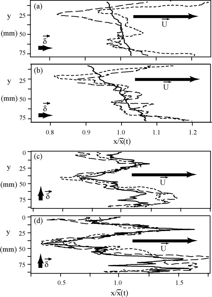
Experimental isoconcentration fronts (c = 0.5) in model 3 (graphs (a) and (b)) and in model 4 (graphs (c) and (d)) as a function of the normalized distance $x \bar{(x (t)}$ ( $\bar{x} = mean front distance$ ) for two different ratios β of the injected volume to the pore volume (dots: β = 0.85, dashes: β = 0.5). Mean velocities: (a), (c): U = 0.0125 mm/s, Pe = 14; (b), (d): U = 0.25 mm/s, Pe = 285. Continuous line: theoretical variation from Eq. (4). All experiments have been realized with identical 1000 ppm water-polymer solutions.
Fronts isoconcentrations expérimentaux (c = 0.5) dans le modèle 3 (graphiques (a) et (b)) et dans le 4 (graphiques (c) and (d)) en fonction de la distance normalisée $x / \bar{(x (t)} \bar{(x (t)} = distance moyenne du front)$ pour deux rapports différents β du volume injecté et du volume poreux (pointillés : β = 0,85, tirets : β = 0,5). Vitesses moyennes - (a), (c) : U = 0,0125 mm/s, Pe = 14 ; (b), (d) : U = 0,25 mm/s, Pe = 285. Ligne continue : variation théorique d’après l’Éq. (4). Toutes les expériences ont été réalisées avec des solutions eau-polymère identiques de concentration 1000 ppm.

To conclude, in model 3 with $\vec{δ} | | \vec{U}$ , dispersion is mostly controlled by the Taylor dispersivity component due to the velocity profile between the walls as soon as Pe ≳ 12; there is, however, an amplification of the dispersion due to the fracture roughness.

3.4 Fracture model 4

In model 3, the mean flow was perpendicular to the channels or to the ridges induced by the shear displacement: the correlation length of the velocity is then determined by the typical width of these structures. Model 4 has the same size as model 3, a same mean aperture and complementary rough walls with a self-affine geometry exactly identical to that used for model 3. However, the shear $\vec{δ}$ is, this time, perpendicular to the mean flow $\vec{U}$ . In this configuration $(\vec{δ} ⊥ \vec{U})$ , $\vec{U}$ is parallel to the channels and ridges created by the shear: the correlation length of the flow velocity is then determined by the length of the channels which is much larger than their width.

The dispersion characteristics are then very different as can be seen by comparing isoconcentration fronts obtained for model 4 (Figs. 5c, d) and model 3 (Figs. 5a, b) at different times and in identical experimental conditions. More precisely, large fingers and troughs are observed for model 4 while none appears for model 3 (note that the horizontal scales is 3 times more expanded for model 3 than for model 4 in Fig. 5). Also, the amplitude of these features parallel to $\vec{U}$ is larger at the higher velocity for which the solution has a shear-thinning behaviour (Fig. 5d) than at the lower velocity at which it behaves like a Newtonian fluid (Fig. 5d). Another important feature is the good collapse of the large features of the front observed at different times when normalized by the mean distance: this shows that the size of these features parallel to the flow increases linearly with time.

These results show that front spreading is purely convective and that the total width Δx of the front parallel to $\vec{U}$ (i.e. the distance between the tips of the fingers and the bottom of the troughs) increases linearly with distance as xΔU/U (ΔU/U = typical large scale velocity contrast between the different channels created by the shear).

In order to predict these contrasts, we modelled the fracture aperture field as a set of independent parallel channels of aperture a(y) = <a(x,y)>_x ((Auradou et al., 2006; Auradou et al., 2008)). A particle starting at a transverse distance y at the inlet is assumed to move at a velocity proportional to a(y)^(n+1)/n; The theoretical profile x_f (y,t) of the front at a time t is then:

x_{f} (y, t) = \frac{\bar{x (t)} a {(y)}^{(n + 1) / n}}{< a {(y)}^{(n + 1) / n} >_{y}},

(4)

where

\bar{x (t)} = < x_{f} (y, t) >_{y}

and

< a {(y)}^{(n + 1) / n} >_{y}

are averages over y of the local aperture a(x,y). Normalized profiles

x_{f} (y, t) / \bar{x (t)}

computed using Eq. (4) and the actual aperture fields are plotted in Fig. 5a to d as continuous lines. The exponent n has been taken equal to 1 at the lowest velocity for which

\dot{γ} \sim {\dot{γ}}_{0}

(Fig. 5a, c) and to 0.26 at the highest one for which

\dot{γ} > {\dot{γ}}_{0}

(Fig. 5b, d) (as mentioned in Section 2.2,

{\dot{γ}}_{0}

is the shear-rate value corresponding to the crossover from the Newtonian to the shear-thinning behaviour of the fluid).

Eq. (4) clearly predicts well the location and shape of the large “fingers” and “troughs” at both velocities for $\vec{δ} ⊥ \vec{U}$ . In contrast, the theoretical curve does not reproduce the front geometries in model 3 $(\vec{δ} | | \vec{U})$ except for the small global slope.

This confirms that, for $\vec{δ} ⊥ \vec{U}$ (model 4), the large scale features of solute transport are determined by the velocity contrasts between the channels created by the shear. The curves of Fig. 5c, d also reproduce well the difference between the sizes of the fingers at the two velocities investigated. This confirms that the difference between these sizes may be accounted for by the different rheological behavior of the fluid: the velocity contrasts (and, therefore, the size) are amplified for Pe = 285 (shear-thinning power law domain) compared to the vicinity of the Newtonian constant viscosity regime (Pe = 14).

For model 3, the hypothesis of the model are not satisfied and it does not reproduce the front geometry: however, the features of the front are generally visible at similar transverse distances y in Fig. 5a and b (at a given time). They likely reflect also, in this case, a convective spreading of the front due to velocity contrasts between the flow paths: however, there is no simple relation of the front geometry to the aperture field, in contrast with model 4.

One finds the same contrast with model 3 for the variations with time of the concentration displayed in Fig. 3. The time variation of the average $\bar{C} (x, t)$ of the concentration across the model is not well fitted this time (× symbols) by the solutions of Eq. (1). The broad width of the transition zone in the curve and its complex shape reflect the large scale velocity contrasts between the different channels. The variations of the local concentration on single pixels, in contrast, are generally well fitted by solutions of Eq. (1) and, at some points (x,y), the curves are very similar to those obtained for model 3, as can be seen in the inset of Fig. 3. The distribution of the local dispersivity l_d(x,y) is, however, much broader than for model 3 and the mean value is larger.

The same measurements have been performed (Boschan et al., 2007) on model 5 which has a similar wall geometry but corresponds to a smaller amplitude δ = 0.33 mm of the shear (still with $\vec{δ} \vec{U}$ ). In this case, the values of the local dispersivity are very close to those predicted from Taylor dispersion. The amplitude of the large scale fingers is also significantly smaller but their geometry is again well described by Eq. (4) (Auradou et al., 2008). Both features indicate that the disorder of the flow field is stronger for model 4 than for model 5 and, therefore, increases with the amplitude of the displacement δ.

4 Conclusion

To conclude, the present experiments in 5 different models of rough fractures demonstrate that tracer dispersion depends crucially on the geometrical characteristics of the roughness. Investigating the dependence on the Péclet number and the influence of the fluid rheology allows one to identify the different mechanisms and their relative magnitude. The characteristics obtained with the different models can be grouped into two sets.

Models 1 and 2: both models correspond to obstacles with a single characteristic size. The height of the obstacles is smaller than the aperture for model 1 and equal to it in model 2: this models the case of gouge (or proppant) particles bridging the gap. In both cases, the size of the wall rugosities and the correlation length of the velocity field are small compared to the global size of the fracture. As a result, the variation with distance and time of the tracer concentration satisfies the convection dispersion equation (1); moreover, the corresponding values of D are independent of the fraction of the width of the model over which the concentration is averaged and of the distance from the inlet. Dispersion in these models may therefore be characterized by a single macroscopic dispersion coefficient.

At low Péclet numbers, one has, for both models, D ∝ U corresponding to geometrical dispersion due to the disorder of the velocity; in this regime, l_d = D/U increases with the polymer concentration (i.e. with the shear-thinning character of the fluids) due to an enhancement of the velocity contrasts. Moreover, for model 1, the value of l_d is close to that predicted from a small perturbation theory.

At higher Pe's, other characteristics of the structure of the void space such as the flow profile in the aperture (model 1) and the distribution of the tracer in the pore junctions (model 2) influence dispersion. For model 1, there is a transition towards Taylor dispersion with D ∝ Pe². In model 2, D increases at high Pe values as Pe^1.35: this exponent agrees with previous numerical simulations (Bruderer and Bernabé, 2001) and should depend on the distribution of the size of the obstacles. In this latter model, the transition between the different regimes is controlled by mixing at the scale of individual junctions.

Models 3, 4 and 5: The roughness of the walls of these models has a multiscale self-affine geometry similar to that of many fractured rocks; the walls of these fractures are complementary with a relative shear displacement either parallel $(\vec{δ} | | \vec{U})$ for model 3 or perpendicular $(\vec{δ} ⊥ \vec{U})$ for models 4 and 5. The relative shear produces a channelization perpendicular to $\vec{δ}$ of the aperture field: this channelization has a key influence on dispersion which, therefore, depends strongly on the relative orientation of $\vec{δ}$ and $\vec{U}$ .

For $(\vec{δ} ⊥ \vec{U})$ (models 4 and 5), the global spreading of the mixing front is not dispersive: instead, its global width parallel to $\vec{U}$ increases linearly with time and reflects the velocity contrasts between the channels. For the largest relative shear δ = 0.75 mm (model 4), large scale structures of the front can be predicted from the aperture field and their size increases with the shear-thinning character of the fluid.

The variation of the local thickness of the front remains instead dispersive: for the smaller relative shear δ = 0.33 mm (model 5), the value of D corresponds to Taylor dispersion while, for model 4, it is larger.

For model 3 $(\vec{δ} | | \vec{U})$ , the global spreading of the front is much weaker that in model 4 of same characteristics but for which $\vec{δ} ⊥ \vec{U}$ : local spreading is controlled by Taylor dispersion at large Pe's and by molecular diffusion at lower ones. Actually, for models 3,4,5, no geometrical dispersion regime is observed, even at low Péclet numbers.

An important issue in the channelized fractures is whether the transverse exchange of tracer may be large enough so that a diffusive spreading regime is reached at very large distances. Recent work by other authors (Bauget and Fourar, 2008) report adjustments of dispersion curves in rough sandstone samples by a similar parallel channels model: however, the adjusted parameters vary in this case with the distance from the inlet. This may indeed result from some amount of transverse exchange reducing the channelization effect.

These results have a strong relevance to the efficiency of the recovery of heat through water circulation in geothermal reservoirs. There are also other possible applications to the prediction of seismic events from water circulation in the rock layers under stress.

Acknowledgments

We are indebted to R. Pidoux for his assistance. HA and JPH are supported by CNRS through GdR No. 2990) and by the European Community (STREP EGS PILOT PLANT - EC Contract SES-CT-2003-502706). This work was greatly facilitated by a CNRS-Conicet Collaborative Research Grant and by the Ecos Sud A03E02 program.

Bibliographie

[Adler and Thovert, 1999] P.M. Adler; J.-F. Thovert Fractures and Fracture Networks, Kluwer Academic Publishers, Dordrecht, The Netherlands, 1999 ([444 p.])

[Auradou et al., 2005] H. Auradou; G. Drazer; J.P. Hulin; J. Koplik Permeability anisotropy induced by a shear displacement of rough fractured walls, Water Resour. Res., Volume 40 (2005), p. W09423

[Auradou et al., 2006] H. Auradou; G. Drazer; A. Boschan; J.P. Hulin; J. Koplik Shear displacement induced channelization in a single fracture, Geothermics, Volume 35 (2006), pp. 576-588

[Auradou et al., 2008] H. Auradou; A. Boschan; R. Chertcoff; S. Gabbanelli; J.P. Hulin; I. Ippolito Enhancement of velocity contrasts by shear-thinning solutions flowing in a rough fracture, J. Non-Newtonian Fluid Mech., Volume 153 (2008), pp. 53-61

[Bauget and Fourar, 2008] F. Bauget; M. Fourar Non-Fickian dispersion in a single fracture, J. Cont. Hydr., Volume 100 (2008), pp. 137-148

[Bear, 1972] J. Bear Dynamics of Fluids in Porous Media, Elsevier Publishing Co, New York, USA, 1972 ([764 p.])

[Bijeljic and Blunt, 2006] B. Bijeljic; M.J. Blunt Pore-scale modeling and continuous time random walk analysis of dispersion in porous media, Water Resour. Res., Volume 42 (2006), p. W01202

[Boschan et al., 2007] A. Boschan; H. Auradou; I. Ippolito; R. Chertcoff; J.P. Hulin Miscible displacement fronts of shear thinning fluids inside rough fractures, Water Resour. Res., Volume 43 (2007), p. W03438

[Boschan et al., 2008] A. Boschan; I. Ippolito; R. Chertcoff; H. Auradou; L. Talon; J.P. Hulin Geometrical and Taylor dispersion in a fracture with random obstacles: An experimental study with fluids of different rheology, Water Resour. Res., Volume 44 (2008), p. W06420

[Brown et al., 1998] S. Brown; A. Caprihan; R. Hardy Experimental observation of fluid flow channels in a single fracture, J. Geo. Res., Volume 103 (1998), pp. 5125-5132

[Bruderer and Bernabé, 2001] C. Bruderer; Y. Bernabé Network modeling of dispersion: Transition from Taylor dispersion in homogeneous networks to mechanical dispersion in very heterogeneous ones, Water Resour. Res., Volume 37 (2001), pp. 897-908

[D’Angelo et al., 2007] M.V. D’Angelo; H. Auradou; C. Allain; J.P. Hulin Pore scale mixing and macroscopic solute dispersion regimes in polymer flows inside two-dimensional model networks, Phys. of Fluids, Volume 19 (2007), p. 033103 | DOI

[Detwiler et al., 2000] R. Detwiler; H. Rajaram; R.J. Glass Solute transport in variable aperture fractures: An investigation of the relative importance of Taylor dispersion and macrodispersion, Water Resour. Res., Volume 36 (2000), pp. 1611-1625

[Gelhar, 1986] L.W. Gelhar Stochastic subsurface hydrology: from theory to applications, Water Resour. Res., Volume 22 (1986), p. 135S-145S

[Genter et al., 1997] A. Genter; C. Castaing; Ch. Dezayes; H. Tenzer; H. Traineau; T. Villemin Comparative analysis of direct (core) and indirect (borehole imaging tools) collection of fracture data in the Hot Dry Rock Soultz reservoir (France), J. Geophys. Res., Volume 102 (1997), pp. 15419-15431

[Gentier et al., 1997] S. Gentier; E. Lamontagne; G. Archambault; J. Riss Anisotropy of flow in a fracture undergoing shear and its relationship to the direction of shearing and injection pressure, Int. J. Rock Mech. Min. Sci., Volume 34 (1997), p. 412

[Ippolito et al., 1993] I. Ippolito; E.J. Hinch; G. Daccord; J.P. Hulin Tracer dispersion in 2-D fractures with flat and rough walls in a radial flow geometry, Phys. Fluids A, Volume 5 (1993), pp. 1952-1961

[Keller et al., 1999] A.A. Keller; P.V. Roberts; M.J. Blunt Effect of fracture aperture variations on the dispersion of contaminants, Water Resour. Res., Volume 35 (1999), pp. 55-63

[Lee et al., 2003] J. Lee; J.M. Kang; J. Choe Experimental analysis on the effects of variable apertures on tracer transport, Water Resour. Res., Volume 39 (2003), p. 1015 | DOI

[Matsuki et al., 2006] K. Matsuki; Y. Chida; K. Sakaguchi; P.W.J. Glover Size effect on aperture and permeability of a fracture as estimated in large synthetic fractures, Int. J. Rock Mech. Min. Sci., Volume 43 (2006), pp. 726-755

[NAS Committee, 1996] NAS Committee on Fracture Characterization and Fluid Flow, Rock Fractures and Fluid Flow: Contemporary Understanding and Applications, National Academy Press, Washington, D.C, USA, 1996, 551 p.

[Neretnieks et al., 1982] I. Neretnieks; T. Eriksen; P. Tahtinen Tracer movement in a single fissure in granite rock: Some experimental results and their interpretation, Water Resour. Res., Volume 18 (1982), pp. 849-858

[Park et al., 1997] C.-K. Park; T. Vandergraaf; D. Drew; P.-S. Hahn Analysis of the migration of nonsorbing tracers in a natural fracture in granite using a variable aperture channel model, J. Cont. Hydr., Volume 26 (1997), pp. 97-108

[Park et al., 2001] Y. Park; J.R. de Dreuzy; K. Lee; B. Berkowitz Transport and intersection mixing in random fracture networks with power law length distributions, Water Resour. Res., Volume 37 (2001), pp. 2493-2502

[Roux et al., 1998] S. Roux; F. Plouraboué; J.P. Hulin Tracer dispersion in rough open cracks, Transport Porous Media, Volume 32 (1998), pp. 97-116

[Sausse, 2002] J. Sausse Hydromechanical properties and alteration of natural fracture surfaces in the Soultz granite (Bas-Rhin,France), Tectonophysics, Volume 348 (2002), pp. 169-185

[Tsang and Tsang, 1989] Y.W. Tsang; C.F. Tsang Flow channeling in a single fracture as a two-dimensional strongly heterogeneous permeable medium, Water Resour. Res., Volume 25 (1989), pp. 2076-2080

Commentaires - Politique

Ces articles pourraient vous intéresser

The influence of spatial variability on 2D reactive transport simulations

Marco De Lucia; Vincent Lagneau; Chantal de Fouquet; ...

C. R. Géos (2011)

Impact of the fracture contact area on macro-dispersion in single rough fractures

Anthony Beaudoin; Mohamad Farhat

C. R. Méca (2021)

Equivalent block transmissivity in an irregular 2D polygonal grid for one-phase flow: A sensitivity analysis

Marco De Lucia; Chantal de Fouquet; Vincent Lagneau; ...

C. R. Géos (2009)