

1 Introduction
The Pan-African North Equatorial region is very sensitive to the distribution of precipitation determined by the seasonal and interannual variations of the Intertropical Convergence Zone (ITCZ). Today, the southern part of the region extending from 5°S to 25°N and from 18°W to 35°E is under the influence of the African monsoon climate (Fig. 1). The core of the rainbelt is located around 10°N during summer (JJAS), during which the Sahelian region further north receives its annual amount of precipitation. The northern part of the region is under desert climate with sporadic low annual rainfall (< 50 mm/year in average and up to 200 mm/year maximum in northern Chad). Therefore, the distribution of vegetation in this region is constrained by water availability, as attested by the zonal distribution from forest in the south to desert in the north. The Sahel region is particularly vulnerable to changes in the hydrological cycle, and there is still much uncertainty about the future evolution of water resources [22]. There is thus a need to better understand how the vegetation and hydrology respond to long-term climate fluctuations, and what their complex interactions are.
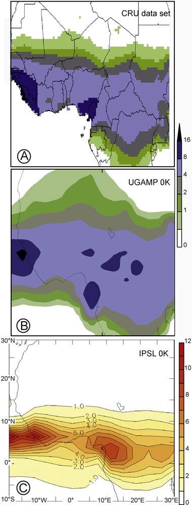
Present-day patterns of the summer African monsoon (JJAS), with rainfall in mm/day. A) Observed precipitation extracted from the Climate Research Unit [40], B) simulated daily precipitation from the slab Ocean-Atmosphere GCM UGAMP [18], and C) simulated daily precipitation from the coupled Ocean-Atmosphere GCM IPSL [36].
Fig. 1. Patron des précipitations estivales (JJAS, en mm/jour) de la Mousson africaine actuelle. A) Valeurs observées extraites de l’Unité de recherche sur le climat (CRU, [40]), B) valeurs simulées à partir du modèle atmosphérique UGAMP (océan prescrit, [18]) et C valeurs simulées à partir du modèle couplé océan-atmosphère IPSL [36].
Past climate indicators show that this region experienced large changes in the hydrological cycle and the vegetation during the Holocene. In particular, lake level, pollen, and other macrofossil data suggest that this area was moister and the vegetation cover, including grasses and trees, was denser during the first half of the Holocene than today [e.g. 23]. Data analyses and modelling studies have shown that these changes are linked to changes in insolation resulting from the long-term variations of the Earth's orbital parameters. In particular, a decrease in obliquity during the Holocene, which affected the latitudinal temperature gradients, and precession led to a 180° shift of the location of the vernal equinox on the Earth's orbit during the Early Holocene, so that the seasonal cycle of insolation was enhanced in the Northern Hemisphere and damped in the Southern Hemisphere at that time. Changes in the precession during the Holocene alter the shape and the amplitude of the seasonal cycle as well as the length of the seasons [8,24]. Because of the enhanced seasonal cycle of insolation, both the interhemispheric and the land-sea temperature gradients were enhanced during boreal summer, which favoured the inland penetration of the monsoon flow and produced high summer precipitation in regions that are now arid in the Sahel and Sahara [12,25]. However, model-data comparisons of the Mid Holocene performed as part of the Paleoclimate Modeling Intercomparison Project (PMIP) show that most models simulate an enhanced monsoon at that time, but that they fail to produce the amount of precipitation needed to sustain any vegetation as far as 23°N [7,19,25]. This drawback is a combination of systematic model biases that lead to an incorrect location of the monsoon rain belts over the continent, and of deficiencies in producing the right sensitivity of the hydrological cycle to the insolation forcing. Moreover, several studies have shown that the response of the ocean and of the vegetation to the Mid-Holocene insolation forcing both contribute to enhance the monsoon flow by positive feedbacks to the atmosphere [5].
Some paleo records suggest a rapid termination of this moist period (called the African humid period, AHP) after 5500 yr BP [13]. This abrupt shift from moist to arid conditions resulted from seasonal, as well as interannual and long-term, climate changes (ocean, soil humidity) caused by external forcing such as from Earth orbital parameters. Simulations with intermediate complexity models indicate that the vegetation feedback had a major contribution in the end of the AHP [11,32,47], while simulations with General Circulation Models (GCM) suggest that the rapid change in the vegetation is caused by a non-linear response of vegetation threshold in the presence of high climate variability [33]. Differences in the proposed mechanisms may result in part from the representation of vegetation in the models, or from differences in the representation of interactions between the land surface and the atmosphere. Although the different simulations provide possible reasons for a rapid decrease in precipitation (ending the AHP), they do not consider in detail the different vegetation types and the fine-scale distribution of vegetation that may explain why the end of the AHP is not recorded simultaneously in pollen assemblages across the whole region [13,27,39,49]. There is thus a need to better understand the evolution of past vegetation as seen from the pollen records.
In this article, we focus on the vegetation and its evolution through the Holocene using the analysis of several time slices including the Early Holocene (between 10 K and 9 K BP), Mid-Holocene (6 K BP), the end of the African humid period (4 K BP) and the present day (0 K BP). Our objective is to analyze the response of a dynamical vegetation model to the climate changes simulated by two different GCMs. This analysis represents a first step towards a better understanding of the distribution of vegetation through time in West Africa. In addition, the comparison of the vegetation model output with pollen assemblage data is an important step to evaluate vegetation simulations and to refine the possible reasons for the observed changes.
We present in section 2, the two GCMs and their Holocene simulations used to force in an “off-line mode” the vegetation model LPJ-GUESS. Pollen data sets and the LPJ-GUESS model are presented in section 3. The simulated vegetation results are presented and discussed in section 4, focusing first on the simulations and then on the comparison with the pollen assemblages and other proxies from the four following sub-regions: eastern Sahara, western Sahara, the transcontinental latitudinal region of Sahel, and the equatorial rainforest region near the Gulf of Guinea.
2 Climate models, simulations, and continental-scale changes
2.1 Climate models and simulations
Our goal here is to go beyond these continental-scale changes and see how regional-scale vegetation, both simulated from model and reconstructed from pollen, responds to changes in insolation and related changes in precipitation during the Holocene. We use the Climate Research Unit (CRU) time-series data set at 0.5° spatial resolution [38] as the modern observed reference climate. For the Holocene, we use the results of two different climate models for which simulations of several key periods in the Holocene are available. This allows us to consider the uncertainty resulting from climate model formulation, in our vegetation simulations [25].
The first set of experiments was run with the Atmosphere-slab ocean GCM UGAMP model [18]. The periods considered are 10 K, 9 K, 6 K, 4 K BP, and 0 K (pre-industrial control) and the results of the simulations were downloaded from the University of Bristol. The second set of experiments was run using the IPSL-CM4 coupled ocean-atmosphere model [36]. The model was run for 6 K and 0 K as part of PMIP [6,7], and run for 9.5 K and 4 K (beginning of the African Humid Period, and beginning of its end, respectively) for this study. Early and Mid-Holocene simulations are discussed in Marzin and Braconnot [37] and in Braconnot et al. [8]. All the simulations consider changes in the incoming solar radiation at the top of the atmosphere resulting from the long-term changes in the Earth's orbital parameters. The parameters were prescribed following Berger [2]. In the case of the UGAMP model, small changes in the atmospheric CO2 concentration are also considered, but they account only for a small forcing, since the CO2 varies between 263 to 280 ppmv during the Holocene.
2.2 Downscaling correction
Since we would like to simulate a vegetation cover that is not greatly affected by internal model biases, a downscaling correction is applied to the simulated climate. Indeed, the two models reproduce the different aspects of the African monsoon climatology, but the simulated precipitation for modern day suffers from systematic differences with modern climatology (Fig. 1). The IPSL model tends to underestimate the northward inland penetration of the monsoon belt, whereas the UGAMP model overestimates it.
For each Holocene period, the downscaling correction consists first in computing GCM climate anomalies between the Holocene GCM simulation and the present-day GCM control simulation to infer the climate changes for the mean climatology (12 months of the year). The last decades of the corresponding simulations are used to have a robust estimate. For temperature, the difference between the two periods is considered, while the percentages of change are considered for precipitation and cloud amount, following what was done in previous studies [1,23,45,46]. These anomalies are then downscaled on the finer CRU grid of 0.5 × 0.5° that is more compatible for comparison with local proxy records [23,46]. For each climate variable, the anomaly at each CRU grid point is obtained by a distance weighted average of the anomalies computed for the nearest GCM grid points. This anomaly is added to the CRU climatology to reconstruct the mean climate of the paleo period. Since we also need to specify the interannual climate variability as an input of the LPJ model, we reconstruct 100-years time series for each climate variable and at each CRU grid point using information on the interannual variance. For UGAMP, we use the modern variance, since this variable is not available for the paleo simulations. For IPSL we compute the percentage of change of variance between the two climates, and downscale it on the CRU grid, as it is done for the mean climatology. A normal distribution for temperature, a gamma distribution for precipitation [40], and a beta distribution for cloud cover percentage are used in combination with the mean climatology to construct a 100-years time series for each month and each variable [46]. The daily meteorology within each month is obtained through the LPJ weather generator as is done to simulate the modern vegetation using the CRU data.
It is important to keep in mind that another methodology could have led to slightly different results. In particular, using only the departure from climatology for the precipitation field simulated with the IPSL model would produce smaller changes in vegetation at the limit between steppe and desert vegetation. However, the downscaling correction method we use only affects the mean climate, but does not alter relative changes across Africa for a given period or between the different periods.
2.3 Continental-scale climate changes across the Holocene
The continental-scale analysis shows that summer rainfall simulated during the Holocene was more important than today for both models (Fig. 2), but due to internal differences, IPSL and UGAMP simulate differently the African Humid Period in terms of timing, duration, and spatial pattern. The IPSL climate model shows a continuous drying trend over time from Early to Late Holocene with intensified aridity occurring between 4 K BP and today, while the UGAMP climate model first simulates increased humidity during the Early to Mid-Holocene followed by a shift to arid condition after 6 K BP, and with intensified drying during the Late Holocene.
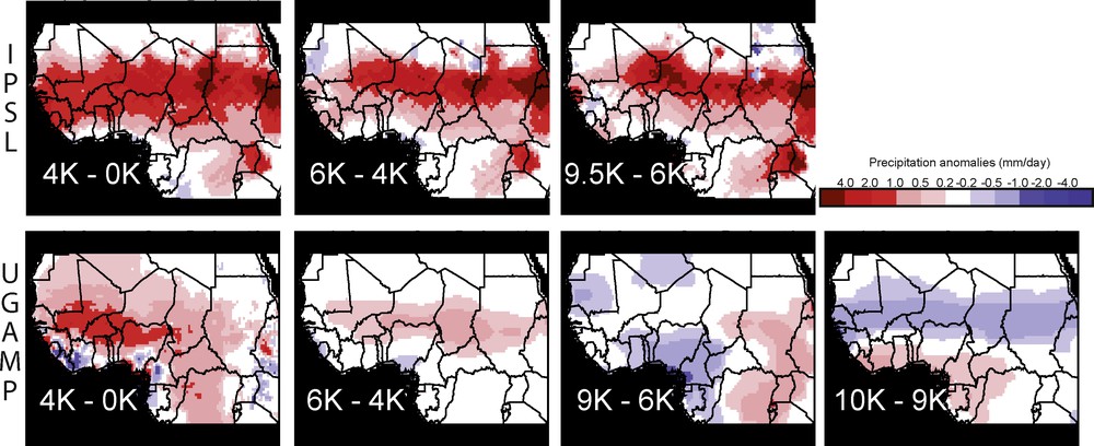
Regional monsoon pattern changes between consecutive periods during the African Humid Period based on IPSL (top) and UGAMP (bottom) GCM. Precipitation anomalies are in mm/day.
Fig. 2. Changements des patrons régionaux de la mousson entre deux périodes consécutives durant la Période Humide Africaine selon les GCM IPSL (haut) et UGAMP (bas). Les anomalies des précipitations sont en mm/jour.
The IPSL CRU-corrected precipitation clearly shows that the large wet area distributed over the Sahel region has been drying from 9.5 K to the present, with a precipitation anomaly reaching up to 4 mm/day in some places (Fig. 2 top). These changes may be artificially high due to the correction applied in regions where the IPSL climate model underestimates modern precipitation. Outside of this wet Sahelian rain belt drying, small regions, around the Gulf of Guinea in West Africa and in eastern Sahara, were undergoing an increase in the amount of summer precipitation from 9.5 K to 4 K BP, followed by a reverse trend from 4 K BP to now. The overall drying pattern during the Holocene with stable or enhanced precipitation near the Gulf of Guinea and at the equator suggests a southward shift of the ITCZ across the Holocene, or at least a decreasing rain belt width. The AHP simulated by IPSL was therefore already maximum around 9.5 K BP over the central transcontinental Sahelian region, and it regularly dried back to modern condition, whereas this maximum was reached later (Mid- or Late-Holocene) in western Africa and eastern Sahara, with the drying more pronounced and at the continental scale between 4 K and 0 K (Fig. 2).
Precipitation anomalies from the CRU-corrected UGAMP simulations show a slightly different story (Fig. 2 lower). They clearly show that the relative intensification of the African monsoon (the AHP onset) started between 10 K and 9 K BP over semi-arid and arid regions from 10°N to 22°N, including therefore Lake Chad and the Sahelian transcontinental latitudinal region. Conversely, equatorial regions around the Gulf of Guinea recorded drying conditions from 10 K to 9 K BP, which suggests that the ITCZ was narrower or had shifted from 10 K to 9 K BP. Between 9 K and 6 K BP, the ITCZ was strengthened or wider over all western African regions, inducing changes in the spatial distribution of increased rainfall, with southward expansion around the Gulf of Guinea (initiating there the AHP onset and likely the wettest period), northward expansion near the Atlantic Ocean in Mauritania and in Algeria, and roughly stable distribution on the Sahelian transcontinental region. A west-east decreasing humidity gradient was also in place at that time. The southern retreat of monsoon belts after 6K BP due to reduction in insolation is clearly seen through the overall aridity pattern set over the Sahelian region, such aridity being intensified after 4 K BP in terms of amplitude and spatial extent, mainly in the western portion of Sahel. Therefore, UGAMP simulations show that the termination of the AHP had taken place sometime between 6 K and 4 K BP over the Sahel, and likely after 4 K BP elsewhere.
The first part of the Holocene differs between the two models, even though they both suggest that the decrease in precipitation first took place in the eastern part of Africa. Both models show that the end of the AHP is more pronounced in the western part of the area between 4 K and 0 K. Also, since the magnitude and details of the patterns are quite different between the two climate models, the simulated vegetation may be different, but it will help us to isolate which part of the regional response is in better agreement with the reconstructed vegetation from pollen.
3 Vegetation: pollen data and LPJ-GUESS Dynamic Global Vegetation Model
Today, the study area encompasses the main African vegetation zones presented in White [58] (Fig. 3) from equatorial moist tropical rain forests (TRFO) northward to drier forests such as tropical seasonal forests (TSFO), deciduous forests or woodlands (TDFO), Guinean, Sudano-Guinean, and Sudanian savannas (SAVA), Sahelian grasslands or steppes (STEP), and desert (DESE).
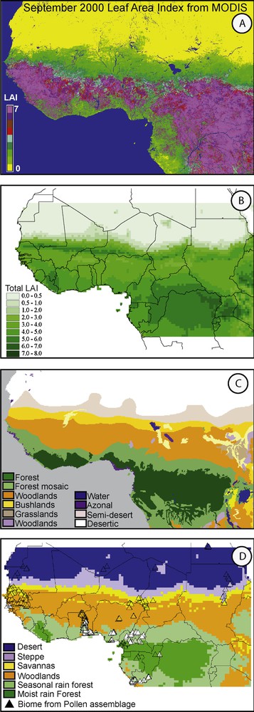
Present-day vegetation characteristics: A) remote sensed LAI product from MODIS (Sept. 2000), B) simulated LAI from LPJ-GUESS using CRU climate data set, C) White [58] vegetation zones from UNESCO (AETFAT/UNSO), and D) vegetation types extracted from the classification from Hély et al. [21] on simulated LAI (reported in panel B) and biomes (triangles) from pollen assemblages extracted from the African Pollen Database for which the biomization method developed by Prentice et al. [44] has been applied [31]. White triangles represent pollen assemblages sampled in the landscape mosaic composed TSFO and SAVA patches reported as the 11a vegetation type in White [58] and used in Lézine et al. [31].
Fig. 3. Caractéristiques de la végétation actuelle : A) d’après l’indice de surface foliaire extrait du satellite MODIS (Sept. 2000), B) d’après les simulations de LPJ-GUESS à partir des données du CRU, C) d’après les zones de végétation de White [58] d’après les données UNESCO (AETFAT:UNSO) et D) d’après les types de végétation de la classification de Hély et al. [21] à partir de l’Indice de Surface Foliaire LAI (reporté dans le panneau B) et d’après les biomes (triangles) reconstruits à partir des assemblages polliniques extraits de la base de données Polliniques Africaines par la méthode de biomization (développée par Prentice et al. [44] et récemment adaptée [31]). Les triangles blancs représentent les échantillons polliniques récoltés dans la mosaïque paysagère composée de TSFO et SAVA incluses (type de végétation 11a selon White [58] et récemment utilisé tel quel dans Lézine et al. [31]).
3.1 Pollen data
The pollen data used for the comparison between pollen biomes and simulated vegetation types [21,31], include 453 terrestrial sites from across the study area (Fig. 3), while the fossil pollen data only include 28 terrestrial sites from 10°N northward, all extracted from the Fossil Pollen Database (http://fpd.mediasfrance.org/). Fossil pollen sites are unevenly distributed throughout West Africa and through time, with 21 sites for 9.5 K BP, among which 13 sites also record pollen data at 6 K BP, and 10 sites still record pollen at 4 K BP. The 6 K BP period is represented by a total of 20 sites, with seven new sites as compared to the 9.5K BP period, and among which only two sites also contain pollen data for the 4 K BP period. We assigned a biome type to all modern and fossil pollen samples using the biomization method originally developed by Prentice et al. [44], and adapted for African vegetation by Vincens et al. [56] and Lézine et al. [31]. The southern-most fossil site included in this study is located around 10.38°N Lake Tilla, [34,50]; therefore, the comparison between simulated vegetation and reconstructed pollen biomes is not performed south to Lake Tilla. However, as we found interesting results from the dense rainforest, this area is also analyzed and discussed based on results from the literature, especially the Dahomey gap region [49].
3.2 LPJ-GUESS Dynamic Global Vegetation Model
In the remainder of the manuscript, we discuss vegetation maps simulated using the LPJ-GUESS model, a generalized ecosystem modelling framework [51,52] based on explicit formulations of the dynamic processes found within an ecosystem, including physiological, biophysical and biogeochemical processes, but also plant population dynamics, competition among plant functional types (PFT), and disturbances. The version used includes improved representations of soil hydrology and atmosphere-vegetation-soil exchange of water [16]. We apply LPJ-GUESS in population mode, which corresponds closely to the global model LPJ-DGVM [51].
The driving variables for LPJ-GUESS are monthly temperature, precipitation and cloudiness, as well as atmospheric CO2 concentrations and a prescribed soil texture class for each grid cell. The model is applied across a 0.5° × 0.5° grid over the study area. Within each grid cell, the vegetation is described as a mixture of PFTs. Each PFT is defined by a set of parameters describing plant physiognomy and allometry, physiology, phenology and bioclimatic limits [51,52]. Within each pixel, LPJ-GUESS is run 1100 years with the first 1000 years corresponding to the spinup period (the first 30 years of the climate time-series are repeated several times). During, the spinup period, all aboveground and soil carbon pools are filled and PFT show dynamics in equilibrium at the end of the spinup with the climate initial input. The entire 100-years time series is then used, inducing or not changes in PFT proportion in terms of Leaf Area Index (LAI), Carbon biomass, Net Primary Production, and fluxes to the Atmosphere.
We have selected the LAI (m2 of leaves/m2 of ground) for comparison, as this variable defines an important structural property of a plant canopy that is used preferentially by ecological and climate modellers who desire a representation of canopy structure (from trees and/or grasses) in their models. LAI increases from 0 in desert regions to 6 or 7 in dense closed-canopy rainforests of evergreen trees (Fig. 3). LAI values reported in the results section represent the averaged annual LAI value over the last 30 years of simulation. We present both total LAI (sum of PFT present in the pixel) and LAI values per PFT to analyze both vegetation structure and composition.
In order to compare simulated vegetation with pollen data that have been biomized, we developed a LAI-vegetation type classification (Table 1) inspired from Hély et al. [21], with calibration using the West-African zones of White [58], and validation using the modern biomes (Fig. 3) reconstructed from pollen sample biomization [31].
Tableau 1 Classification de l’Indice de Surface Foliaire (LAI) simulé par LPJ-GUESS en type de végétation (DESE pour désert, STEP pour steppes ou formations herbeuses du Sahel, SAVA pour savanes, TDFO pour forêts tropicales claires ou décidues, TSFO pour forêts tropicales semi-décidues, et TRFO pour forêts tropicales humides sempervirentes).
| Rule #1 | Rule #2 | Rule #3 | Rule #4 | Rule #5 |
| if Tot. LAI = 0 | DESE | |||
| if Tot. LAI > 0 | and Tot. LAI < 2 | and Tot. LAI < 0.5 | DESE | |
| and Tot. LAI ≥ 0.5 | STEP | |||
| and 2 ≤ Tot. LAI < 4 | and woody LAI = 0 | STEP | ||
| and woody LAI > 0 | and %woody LAI | |||
| < 10% of Tot. LAI | SAVA | |||
| and %woody | ||||
| ≥ 10%of Tot. LAI | TDFO | |||
| and Tot. LAI ≥ 4 | and %TRBE < 60% | |||
| of Tot. LAI | TSFO | |||
| and %TRBE ≥ 60% | ||||
| of Tot. LAI | TRFO |
4 Results
The study area has been divided into four regions based on the increasing influence of the African monsoon pattern from the Sahara desert (western and central-eastern Saharan regions, respectively, due to the influence of the Indian monsoon in eastern Sahara) to the Sahel region with a latitudinal transcontinental band configuration, and to the equatorial forested region. Biomes reconstructed from the GCM-LPJ simulations are presented within such geographical framework, and compared with those inferred from pollen assemblages and other proxies.
4.1 Central – eastern Saharan region (> 10°E and >18°N)
According to the changes in total and PFT LAI provided by the IPSL-LPJ simulations (Fig. 4), steppe vegetation was already present at 9.5 K BP up to the northern boundary of the studied area (LAI ≥ 3 and composed exclusively of C4 grasses at 26°N). These steppes (Sahelian grasslands) have both expanded in area (new grid cells with vegetation present) and increased in structure (increased LAI in grid cells with vegetation present) from 9.5 K to 6 K, with few patches in northern modern Niger and Chad showing increase in tropical raingreen trees (TRBR, leaves out during the rain season) around 19°N. Then, this open-wooded vegetation regressed both in area and structure (lower LAI) at 4 K, with TRBR trees disappearing from Chad but persisting in Niger, before disappearing completely at the present day south to 14°N (northern savanna limit). Meanwhile, only C4 grasses were present in several areas with LAI ≥ 2 at 4K BP, and LAI ≤ 0.5 nowadays. The story is different according to UGAMP-LPJ simulations (Fig. 5), in which the entire region (except northern Chad) remained stable over the AHP to present day with sparse steppe vegetation (LAI ≤ 0.5).
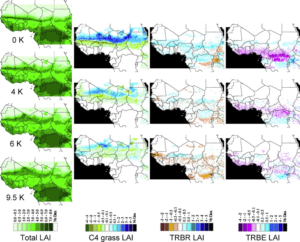
Maps of simulated LAI from LPJ-GUESS using the CRU data set for the modern period (0K BP), and the IPSL climate simulations for 4 K, 6 K, and 9.5 K BP. Maps in the first column represent Annual total Leaf Area Index (LAI) for each period considered, while maps within the three next columns represent the LAI differences from an Early Holocene period to the next one (i.e. 9–6 K, 6–4 K, 4–0 K) for a given PFT (C4 grasses, Tropical deciduous trees (TRBR), and evergreen trees [TRBE]). For these three last columns, blue color always means PFT decrease in the most recent period of the two analyzed, the decrease being more important in darker blue.
Fig. 4. Cartes des LAI simulés par LPJ-GUESS à partir des données du CRU pour la période moderne (0K BP) et des données de IPSL pour 4 K, 6 K, et 9.5 K BP. La première colonne représente le changement du LAI total annuel pour chaque période considérée, alors que les trois autres colonnes représentent la différence de LAI pour chacun des trois PFT (herbacées en C4, arbres tropicaux décidus [TRBR], et ceux sempervirents [TRBE]) entre deux périodes successives. Sur ces cartes, le bleu représente une diminution du PFT analysé dans la période la plus récente des deux, le gradient de couleur étant proportionnel à la diminution du LAI.
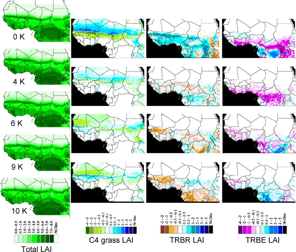
Maps of simulated LAI from LPJ-GUESS using the CRU data set for the modern period (0 K BP), and the UGAMP climate simulations for 4 K, 6 K, 9 K, and 10 K BP, respectively. This figure uses the same rules and legends as Fig. 4.
Fig. 5. Cartes des LAI simulés par LPJ-GUESS à partir des données du CRU pour la période moderne (0 K BP), et des données de UGAMP pour 4 K, 6 K, 9 K, et 10 K BP. Cette figure utilise les mêmes règles et légendes que celles de la Fig. 4.
Reconstructed biomes from pollen data at 9.5 K BP in northern Sudan are savannas and steppe. A desert is reconstructed in northern Chad (Fig. 6). At 6K BP, these both regions presented extended savannas, whereas at 4 K BP the only pollen site available indicated steppe vegetation.
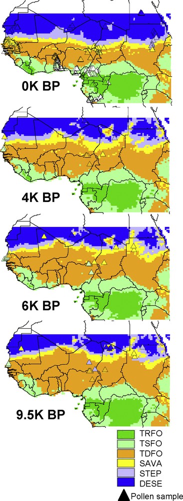
Maps of simulated vegetation types (see Table 1) from LPJ-GUESS using the CRU data set for the modern period (0 K BP), and the IPSL climate simulations for the Holocene. Triangles are representative of biomes reconstructed from pollen samples for the same periods. Pollen biomes at 0 K are the geographically nearest neighbor modern samples available in the APD compared to locations of fossil samples. This figure uses the same rules and legend as Fig. 3D.
Fig. 6. Cartes des types de végétation classifiés (voir Tableau 1) à partir des simulations de LPJ-GUESS utilisant les données du CRU pour l’Actuel et de IPSL pour l’Holocène. Les triangles représentent les biomes polliniques reconstruits à partir des échantillons polliniques pour les périodes considérées. Les biomes polliniques à 0 K BP représentent les échantillons polliniques modernes géographiquement les plus proches du site fossile étudié. Cette figure utilise les mêmes règles et la même légende que la Fig. 3D.
Previous studies using different proxies also noticed the expansion of steppe and savanna into present-day desert. Jolly et al. [23], comparing pollen data and GCM simulations, found that vegetation expanded north up to 23°N from Early to Mid-Holocene, while Neumann [39] found savanna and steppe vegetation to 26°N at 7 K BP in Sudan, with presence of large savanna mammal and archeological remains recorded from 7.5 K BP to 3.7 K BP. Steppe and savanna stopped their northward expansion around Mid-Holocene, and they started their southward gradual retreat due to the termination of the AHP at 4.3 K BP according to Neumann [39] or at 5.2 K BP according to Kröpelin et al. [27]. The southern limit of modern eastern Sahara was reached around 2.7 K BP or 3.3 K BP according to these authors, respectively.
Therefore, the vegetation simulated by IPSL-LPJ (Fig. 6), is in better agreement with pollen data across the AHP than the constant vegetation composition simulated by UGAMP-LPJ (Fig. 7). It provides thus a possible explanation of the timing and evolution of the vegetation in central and eastern Sahara.
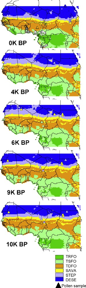
Maps of simulated vegetation types (see Table 1) from LPJ-GUESS using the CRU data set for the modern period (0K BP), and the UGAMP climate simulations for 4 K, 6 K, 9 K, and 10 K BP. This figure uses the same rules and legend as Fig. 6, except for the 9 K and 10 K BP periods for which the same pollen biomes representative of the unique 9.5 K BP time slice have been reported.
Fig. 7. Cartes des types de végétation classifiés (voir Tableau 1) à partir des simulations de LPJ-GUESS utilisant les données du CRU pour l’Actuel et de UGAMP pour l’Holocène. Cette figure utilise les mêmes règles et légendes que la Fig. 6, excepté pour 9 K et 10 K BP où les mêmes biomes polliniques à 9,5 K BP sont utilisés simultanément pour ces deux périodes.
4.2 Western – central Saharan region (< 10°E and >18°N)
According to the IPSL-LPJ simulations, changes in total LAI show that vegetation was at its maximum extent at 9.5 K (Fig. 4) between 18°N and 22°N, dominated by a dense steppe vegetation with savannas in areas where the simulation produces a mean LAI greater than 4 (several pixels with LAI ≥ 5 up to 21°N), mainly composed with C4 grasses and few TRBR trees (Fig. 4, Mali and Algeria). Moreover, sparse steppe with a low vegetation structure (LAI ≤ 1) bordered the northern boundary of the study area, and it was linked to the southern dense steppe and savanna via corridors of steppe with intermediate structure (1 < LAI ≤ 2). At 6 K BP, the simulation suggests through decreasing LAI that area covered by dense steppe has already regressed southwards. Moreover, the few TRBR trees present at 9.5 K BP have disappeared from Mali but grasses were still present (Fig. 4). This southward retreat created steppe patches surrounded by desert on the northern edge. At 4 K BP, the southern regression stopped but grass structure through lowering LAI was still becoming more sparse. The southward regression started again after 4K BP down the present-day southern limit (c. 18°N), where steppe structure is very sparse (LAI < 1). The UGAMP-LPJ simulations also show that western Saharan vegetation has changed through the AHP (Fig. 5), but propose a different evolution compared to IPSL-LPJ simulations. Steppe was the only vegetation type competing with desert progression. Steppe expansion toward the north and west increased from 10 K to 6 K BP, with the spatial distribution of density cover decreasing from south (LAI < 3) to north (LAI < 1). After 6 K BP, the northern limit of sparse steppe (0.5 ≤ LAI ≤ 1) moved 1° southward. After 4 K BP, steppe structure and area kept on regressing southward to the present-day sparse steppe distribution near 18°N.
There are only a few terrestrial pollen sites in western Sahara available for comparison. The only site at 9.5 K BP is located in Mauritania (Fig. 6) and the pollen assemblages were interpreted as savanna vegetation, whereas simulations of both models (Figs. 6 and 7) predicted desert near the northern steppe limit. At 6 K BP, two pollen sites located in northern Mali and southern Algeria reported savanna and desert, respectively. The IPSL-LPJ model simulated a desert for both locations, while the UGAMP-LPJ model simulated a steppe. At 4 K BP, both the pollen site located near the Algeria-Libya boundary and the two model simulations were interpreted as desert, with IPSL simulating more heterogeneous desert-steppe pattern than the homogeneous desert pattern for UGAMP. At a second site in Mauritania, the pollen assemblages were interpreted as a savanna, whereas both models simulated steppes near the southern desert boundary.
There are few studies dealing with continental vegetation reconstructions from the western Sahara. Vegetation simulations from the present study agree with Jolly et al. [23] who report that the southern margin of the western Saharan desert was located around 21°N at least at 9 K BP, whereas at 6K BP this limit was further south, likely located between 15°N and 19°N. Most other studies report vegetation and climate changes from data extracted from offshore marine sediments [13,20,28]. The presence of vegetation in Sahara, resulting from increased summer rainfall from the intensified monsoon during the AHP central phase has been indirectly deduced from the lowered sediment rate [13,53]. Conversely to bare ground, the presence of plants prevented wind erosion and the aerial transport of dust particles.
Therefore, the northward expansion of vegetation into modern desert simulated by both models during the AHP is in fair agreement with pollen data, the UGAMP-LPJ simulations being closer to the limits interpreted from the data than the IPSL-LPJ simulated vegetation. The number of pollen sites is, however, too limited to assess further the realism of the simulations.
4.3 The Sahelian transcontinental latitudinal region (> 12°N and <18°N)
Today, an approximately 500-km wide latitudinal band of semi-arid vegetation crosses Africa (Fig. 4). It is composed of sahelian steppe in the north (LAI ≤ 1.5), sudanian savanna with woody elements in the inner part (2 ≤ LAI ≤ 4) and a woodland on the southern edge of the band (LAI > 4).
According to IPSL-LPJ simulations, this transcontinental region was composed only of savannas and woodlands (2 ≤ LAI ≤ 5) at 9.5 K BP because savannas and steppes had expanded into desert as mentioned above. This spatial distribution changed slightly at 6K BP, when savanna increased in the southern part of the domain against regressing woodlands. This drying pattern continued at 4 K BP, with steppes entering back from the band's northern edge. Aridity likely had accelerated during the 4 K–0 K BP period to produce the modern composition among which steppes and savannas are the most representative of the region.
According to UGAMP-LPJ simulations, vegetation changes differed between the western-central part and the eastern part of this transcontinental region (Fig. 5). The simulation suggests that the width of the latitudinal band in the eastern part has not recorded significant changes during the AHP as compared to present day. Simulated vegetation only recorded a slight northern translation, with the three vegetation types always present. Conversely, the western and central parts have seen their structure and composition changed during the AHP. In the western part, savannas and woodlands, representative of intermediate and high LAI values, have expanded northward from 10 K to 6 K BP pushing steppes out of the transcontinental region from north. Raingreen trees (TRBR) have been responsible for this increase in the western part (between 10 K and 6 K BP), likely because trees could outcompete the C4 grasses due to the increased precipitation brought about by the intensified monsoon. Meanwhile, in the central part of the transcontinental band, only LAI of C4 grasses has increased, likely due to lower added rainfall transport that has maintained TRBR stable and only favored grasses a little bit. After 6 K BP, the climate became drier, allowing steppes to expand southward and to cause savannas and woodlands to regress 100–150 km southward at 4 K BP. The last period between 4 K and 0 K BP exhibited the most intensified drying imposing to steppes, savannas, and woodlands their modern spatial distribution in the transcontinental region.
Several pollen sites, mostly located in the central (mainly Niger, Nigeria, and Chad) and the western (Senegal) parts of the transcontinental region, document the past of this region (Fig. 6). Today, it is covered by savannas, while steppes are interpreted from surface pollen samples on its northern edge, and woodlands and savannas on its southern central edge. Only pollen samples from the south-western Senegal/Guinea-Bissau border reported a more humid vegetation mosaic in the past, composed of savannas and tropical seasonal forest ([58] 11a vegetation zone), whereas both models simulated woodlands and savannas during the entire AHP (Figs. 6 and 7). As compared to the western part, the pollen and simulated vegetation are in better agreement in the central part of the transcontinental region: at 9.5 K BP, woodlands were reconstructed from both model simulations and all pollen assemblages except two. At these two pollen sites, reconstructed vegetation from pollen assemblages was steppes, so that the UGAMP-LPJ simulation better matched the pollen data. At 6 K BP, a wetter climate induced changes to favour moister vegetation types: one steppe was transformed into savanna (the second pollen site with steppe at 9.5 K BP being unavailable at 6 K BP), one woodland became a savanna and another one changed into a tropical seasonal forest, and only two woodlands remained unchanged. Overall, both climate models simulated vegetation patterns in agreement with the interpretations of the pollen data as they both simulated a woodland region with few enclosed savannas, and a seasonal forest located not too far southward. At 4 K BP, except for the two sites where seasonal forests transformed back to woodlands (one located in the transcontinental region and the other one south at Lake Tilla), all sites stayed unchanged as savannas or woodlands. Both simulations agreed with these patterns of change.
4.4 The Equatorial region (> 5°S and <12°N)
Today, this large forested region around the Gulf of Guinea (LAI ≥ 4, Fig. 4) contains two dense closed-canopy rainforests. The western Guinean forest, from Guinea to Togo, encompasses a small area of dense canopy moist rainforest composed exclusively of tropical evergreen trees (TRBE, leaves always out, LAI ≥ 5), surrounded by seasonal rainforest (TRBE + TRBR). The eastern Congolian forest, being representative of the main African tropical rainforest core (5 ≤ LAI ≤ 7), has the same composition as the western forest and spans from Nigeria to the southern limit of the studied area. These two rainforests are separated together by the Dahomey gap (Benin and western Nigeria), named according to the landscape being a mixture of woodlands and savannas [49], where the LPJ-GUESS simulation produces TRBE, TRBR and C4 grasses that present an overall lower structure (LAI < 4) than forests. This gap between both forests is not driven by a topography change but seems to originate from different climate conditions and response of vegetation dynamics.
According to IPSL-LPJ (Fig. 4), the two forests have always been separated since 9.5 K BP, with the widest open area between them at 9.5 K BP. The Guinean forest was only composed of seasonal rainforest (4 < LAI < 5), whereas the Congolian forest was composed both with peripheral seasonal rainforest and moist rainforest in its core. At 6 K BP, some areas in the Guinean forest changed to moist rainforest, and woodlands had regressed from the gap edges, leaving space for new Congolian seasonal rainforest patches. At 4 K BP, these patches of seasonal rainforest previously isolated from the western edge of the Congolian forest were aggregated to the core forest, and seashore vegetation (likely mangroves) had filled the gap on the ocean coast, reducing therefore the width of the woodlands still present in Benin and Nigeria. Only the size of the inner moist rainforest in the Guinean forest slightly increased, and kept on increasing after 4 K BP up to modern distribution, whereas the Congolian forest core slightly regressed in size from its southern edge.
Conversely, according to UGAMP-LPJ (Fig. 5), the two forests have been aggregated as one large forested region at least from 10 K to 4 K. This huge forest included one seasonal rainforest with inside two embedded moist rainforests: the western rainforest located as the present day one, and the eastern one more widespread than today. At 9 K BP, both the seasonal rainforest and the western moist rainforest area had regressed southward from their northern limits becoming more fragmented, and open vegetation areas such as woodlands, savannas, and steppes had appeared from Ivory Coast to Benin coasts. At 6 K BP, these open vegetation areas from Ghana to Benin were still present, whereas the northwestern edge of the seasonal rainforest had expanded back northward from the northern border of Guinea to inside Mali. Simultaneously, rainforest at the western border of Cameroon became isolated from the Congolian rainforest core, which experienced reduction of one LAI unit in canopy structure. At 4 K BP, the open areas in the seasonal rainforest had regressed back in size, and rainforest areas had expanded again, the Guinean part showing its maximum size over the AHP, and the Congolian part being in only one piece again. Therefore, the present day open corridor of the Dahomey Gap between the two forests must have appeared after 4K BP such as demonstrated by Salzmann and Hoelzmann [49].
Simulated vegetation changes through the AHP are only discussed in regards to literature review and not compared to reconstructed pollen biomes. The overall equatorial and subtropical African rainforest has been studied from different areas. From terrestrial studies point of view, it has been analyzed from its northern limit (e.g. Runge [48] and Beuning et al. [4] for Congolian and Guinean forests, respectively) to its core domain [35] and its southern boundary [54]. The rainforest has also been analyzed through the analysis of pollen in marine cores offshore of the Gulf of Guinea [e.g. 14,29]. The main core of moist rainforest has been stable during the AHP, even though species composition may have fluctuated [34,35]. Other rainforest areas in the Guinean region and near the northern savanna-forest limit have recorded progression and regression phases since the AHP onset up to its termination, with the most important regressions and replacements by more open vegetation in areas where forest was more fragile or unstable due to local edaphic and hydrological constraining conditions [48,54,55]. Several authors [e.g. 4,15,29,54] also noted that local conditions may also have delayed forest composition change, inducing a time lag response in vegetation composition change to climate change. Among these sensitive areas, the Dahomey Gap is a good example of vegetation composition changes through the AHP [49], with the final disappearance of seasonal forest and expansion of savannas within less than thousand years (4.5–3.2 K BP), marking the demise of the AHP in that region.
5 Discussion and conclusion
In this analysis, we used the climate simulated by two different climate models to infer the changes in vegetation across the Holocene over Africa in a region extending from 5°S to 25°N where precipitation and water availability play a major role in the evolution of the ecosystems. Both models predicted intensified monsoon rainfall during the Holocene as compared to the present-day pattern. They both showed that, in response to the changes in insolation, the region experienced an overall drying over the Holocene. Despite this agreement on the continental scale patterns, the two models produced changes in precipitation that had different timing, regional patterns and magnitude. The IPSL simulations showed that the humid conditions had begun by 9.5 K BP, and that the wettest AHP phase was over (regional climate was already drying), except in few areas such as the Gulf of Guinea and the eastern Sahara where the AHP onset started later. The UGAMP simulations showed that the AHP onset had taken place between 10–9 K BP in the broad transcontinental Sahel region and during the 9–6 K BP period for other regions. As with the simulation based on the IPSL model, the AHP wettest phase simulated by UGAMP also occurred very early in eastern Africa, whereas conversely to IPSL, it occurred during Mid-Holocene elsewhere. Both models also suggested a slightly different response between the eastern and western part of the studied region, with a more gradual early aridification in the East and a later aridification in the West, which was maximum during the last 4000 years. The differences in the response of the two models to the insolation forcing resulted from model biases, as well as from differences in the model sensitivity of the hydrological cycle due to differences in the parameterization of convection, clouds or surface fluxes.
The simulated climates were used to force “off-line” the LPJ-GUESS vegetation model, and the simulated vegetation was then compared to available data from pollen analyses for different regions. Even though there are only few PFTs available for the African continent in LPJ as in most vegetation models, the LAI-vegetation type classification allowed us distinguishing all biomes necessary to describe vegetation changes through time. The level of diversity obtained with such classification based on model PFTs was the same as the diversity obtained using the pollen biomization method. Indeed, the high diversity of pollen taxa is reduced to few pollen PFTs and to even lesser biome types directly comparable with simulated vegetation types.
In the eastern Saharan desert, simulated biomes and their changes obtained using the IPSL climatologies were in better agreement with biomes and changes inferred from pollen assemblages than those interpreted from the UGAMP climate simulations. Therefore, the wettest phase of the AHP likely occurred before 9.5 K in this region and the drying was gradual throughout the Holocene. The response of the UGAMP model followed this pattern of change after 6 K, but the magnitude was not large enough to reconstruct vegetation in good agreement with paleoecological data. This gradual decrease of the African monsoon in the IPSL model follows the gradual decrease seen for the Indian monsoon [37], suggesting that the East-African monsoon varies in phase with the Indian monsoon as it has been reported for modern interannual variability [10]. Several studies using climate proxies such as eolian dusts [9,41] have concluded that the vegetation change from desert to savannas and woodlands during the AHP was the response to enhanced summer monsoon rainfall. Brookes [9] also showed that this summer pattern was associated with enhanced winter rainfall transported by north-western winds coming from the Mediterranean region. The increase in winter monsoon was also supported by the simulations (not shown).
In the western Saharan desert, both model simulations are in fair agreement with the few data available. Therefore this suggests that precipitation increased at the beginning of the Holocene and that the drying started later (at 6 K and 4 K BP for IPSL and UGAMP, respectively). The simulated termination of the AHP after 4 K BP differs from previous studies based on proxies. Indeed, it is simulated as occurring later and arriving more gradually than the early abrupt event at 5.5 K BP suggested by deMenocal et al. [13], at 5K BP by Brookes [9] from western Sahara or Swezey [53] for the entire Sahara, but it is in phase with the 4.5–3 K BP or the 4.3–2.7 K BP gradual termination suggested by Pachur and Hoelzmann [42] or Kröpelin et al. [27], for eastern and central Sahara, respectively. As in the eastern Sahara, the western Sahara is under the influence of several air masses that transport eolian dusts from these remote desert areas into marine sediments [53]. According to Kuhlmann et al. [28], the northern limit of the African Monsoon influence was located between 27° and 30°N in western Sahara during the AHP [28], northern areas being under the North Atlantic climate regime. Therefore the model results suggest that the northward shift of the limit between the two regimes (North Atlantic – Tropical) had regressed early southward according to the IPSL simulations, whereas in the UGAMP simulations the same limit remained longer in the north over the western Saharan region allowing more humid condition there for longer time.
In the transcontinental Sahelian region, although the magnitude of the changes in precipitation simulated by the two models was very different, both climatologies produced simulated vegetation in agreement with pollen data. The overall pattern in this region was first a kind of plateau (from IPSL) or an increase-decrease precipitation trend (from UGAMP) from 9 K to after 6 K BP and then an aridification. The simulated vegetation response from both models was a dominance of woodlands and savannas across the region during the first phase, and the expansion of steppes from north and regression of woodlands in the last phase. However, these vegetation patterns did not include moister vegetation such as tropical seasonal forests reconstructed from pollen biomes. According to several authors, specificities of the transcontinental Sahelian region in terms of landscape, soil, and hydrology, implies that vegetation changes recorded during the AHP from pollen were the result of the overall regional climate change for the vegetation composition changes, highly influenced by the local conditions for the timing of these changes [17,48,50,57]. Despite such specificities, coherent timing patterns for these simulated AHP periods and vegetation patterns have been found in different areas such as dune fields in the Manga Grassland region [57], and Lake Chad and its surroundings [17].
Further south, despite its intensified summer rainfall simulated over the Gulf of Guinea during the AHP, the IPSL simulations produced a prevailing open vegetation in the Dahomey gap during the Holocene, whereas UGAMP simulations produced a shift from forest to more open vegetation such as woodland and savanna after 4 K BP only, which seems closer to the results from proxies [49]. As tropical seasonal rainforests are composed of TRopical Broadleaved Evergreen and Tropical Broadleaved Raingreen trees (TRBE and TRBR, respectively) that withstand no and only few dry months, respectively, the fact that none of these forests was simulated during the AHP based on IPSL climate simulations means that seasonality over the year was likely overestimated by this model. Apart from the Dahomey gap, timing patterns simulated for the three AHP periods over the broad rainforest region were found similar to those found from vegetation and climate proxies in different locations in the Gulf of Guinea and its surroundings [30,35,43,48,54].
There are several sources of uncertainty in our analysis. The use of two different general circulation models provides an idea of the potential range of response resulting from different model formulations. The time slice approach used in this study is not the best method to analyze the vegetation response time because information just before and just after a given time-slice is missing. Results from literature seem to show that in regions where local conditions are simple in terms of topography, soil characteristics, and hydrology, vegetation response should be both synchronous to climate change, and the result of progressive changes punctuated by drastic changes when physiological and ecological thresholds (e.g. species water stress and openness of the canopy for ombrophilous communities, respectively) are exceeded [e.g. 49]. Conversely, in complex local conditions the vegetation response to a climate change event may be modified (delayed or accelerated), as local conditions may act as positive (accelerated) or negative (delayed) feedbacks on vegetation response. The study by Liu et al. [33] who used the FOAM model to simulate the Late Holocene, suggests different timing of the end of the AHP. The resolution of the model and model biases do not allow a full comparison of the results with data, even though, as in our case the simulation is in broad agreement with data when looking at the continental-scale patterns. Simulations with higher resolution models would be required. As with most impact studies, we were obliged to correct and downscale the climate simulated by the general circulation models to produce vegetation field that have a spatial scale compatible with the different pollen records. The correction was substantial for the two models considered here, and may also impact the results. A better simulation of the modern precipitation would then be required to go further in a detailed analysis of the changes across the Holocene in the different regions. Other caveats come from the vegetation model itself. Even though it has hydrological processes, it is quite simple in regards to water cycle and soil properties. We aim at developing new PFT such as scrub or spiny shrubs able to better describe the arid and desert vegetation types representative of Sahelian and Saharan regions.
Our analyses provide an overall view of the termination of the AHP. In particular, this study supports the idea that the drying was more gradual in East Africa from the beginning of the Holocene and more abrupt in West Africa during the second half of the Holocene. Depending on the author, the termination of the AHP has been described as abrupt [e.g. 13,28,49] or more gradual [27,39,26,30]. An interesting suggestion provided from several authors [29,49,54] would be to analyze the climate model time-series simulations for the different periods in terms of dry season regimes to decipher between the total rainfall amount decrease and/or the amplified seasonality. Such an analysis would allow us to check potential internal problems in the GCMs. Such an analysis would also be interesting from the vegetation point of view because changes in vegetation composition and dynamics result both from competition for water between grasses and trees and from dry season length [21].
Acknowledgement
This research was financed by the French National Agency for Research (ANR 06 VMC SAHELP).