

1 Introduction
Thanks to their specialization and quantification capacities and non-destructive character, geophysical methods are often considered to help in implementing point measurements to study hydrological processes. Among them, Electrical Resistivity Tomography (ERT) is a recent but mature geophysical method increasingly popular in environmental and hydrogeological studies [1–3]. ERT is well suited to 2-D and 3-D field data acquisition and interpretation, and can be adapted to various scales. Time-lapse ERT can also be used to monitor changes in electrical resistivity linked to groundwater flows, because they create variations in water content and/or water conductivity. Time-lapse ERT consists in performing an identical ERT survey several times in the same place, before, during, and after the hydrological process under study. In an unsaturated zone, time-lapse ERT is primarily sensitive to water content variations. Most of the time, a decrease of resistivity indicates an infiltration, and an increase indicates an evaporation. In a saturated zone, time-lapse ERT is sensitive to changes in water conductivity. A decrease of electrical resistivity measured by ERT corresponds to an increase in ionic concentration of the groundwater. An increase of electrical resistivity corresponds to a dilution of groundwater. Controlled experiments in tanks [10,20] demonstrated the potential of time-lapse ERT. In the laboratory or in-situ, time-lapse ERT works best with strong contrasts in resistivity values if salt tracers are used or if pollution plumes are monitored [4,19,22]. In natural conditions in the field, resistivity contrasts are often weaker [17] (i.e. variations from 10 to few tens of percent) and obtaining reliable time-lapse ERT results could be a challenge when trying to locate deep infiltration or recharge zones [6]. Although noticeable improvements have occurred in time-lapse ERT, some recent studies also report image reconstruction difficulties, due to the smoothing effect of the algorithm [10,21]. Some time-lapse ERT surveys fail to recover reliable actual resistivity changes because the calculated resistivity model displays resistivity artefacts (increase or decrease of calculated resistivity) where no changes are expected or measured [6]. Severe misinterpretations of time-lapse ERT surveys can occur, leading to erroneous hydrological understanding of pollution plumes, of groundwater recharge or erroneous modelling. Previous authors [6] have suggested that if a shallow surface infiltration or evaporation occurs during an ERT survey, it could be misinterpreted during ERT inversion. These authors [11] have already demonstrated that a variation of actual resistivity in shallow layers can lead to an opposite variation of apparent resistivity at intermediate electrode spacing. This situation could be particularly acute when the ground is composed of a resistive first layer above a more conductive layer, and when shallow rain infiltration (or evaporation) occurs between two measurements in the field. In the example given by Kunetz [11] with a 2-layer ground, a decrease of actual resistivity within the uppermost part (first quarter, thickness h/4) of the first layer of thickness h can produce an increase of apparent resistivity at intermediate electrode spacing distances between 3 h and 20 h. Then, the easiest model obtained by inversion is one that produces an unexpected increase of calculated resistivity.
This article investigates how a variation of actual resistivity with time and at shallow depth can influence time-lapse ERT results and produce resistivity artefacts at depth. In addition, it presents an advanced time-lapse interpretation to reduce and remove those resistivity artefacts. We used numerical modelling, standard and advanced time-lapse inversions based on a classical addition of a priori information. Then we used a field data set exhibiting typical resistivity artefacts obtained with a standard inversion to show how these resistivity artefacts can be removed.
2 Material and methods
To investigate the effect produced by a shallow infiltration on the ERT method, we adopted a classical method with three stages. The first stage is the construction of two scenarios of shallow infiltration and their translation into experimental apparent resistivity synthetic data sets. The second stage is to use a standard inversion procedure for the time-lapse inversion. The last stage is to introduce a priori information to constrain the inversion of apparent resistivity data. Here, this is referred to as “advanced interpretation”.
2.1 Synthetic models
Fig. 1 presents the synthetic models: a background (initial) model and the two superficial infiltration scenarios. One represents a 1-D resistivity model and the second 2-D resistivity model. From the surface down, the background model has three geological layers:
- • the superficial layer has a thickness of 2.5 m and a resistivity of 500 Ohm m in dry periods, similar to a sandy loam layer;
- • the second layer has a thickness of 3 m and a resistivity of 30 Ohm m, similar to clay;
- • the third layer has a resistivity of 500 Ohm m and represents the substratum.
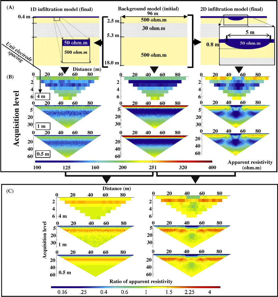
Forward Modelling. (A). Synthetic model. (B). Apparent resistivity model obtained for a Wenner array and three electrode spacings. (C). Ratio of apparent resistivity (final stage divided by initial stage). Note the increase of apparent resistivity at intermediate acquisition levels. The 4-meter spacing data set contains fewer data points (84) than the 0.5-meter spacing data (6048) with a Wenner array.
Modélisation directe. (A). Modèle synthétique. (B). Modèle de résistivité apparente obtenu pour un dispositif Wenner et trois écartements d’électrodes différents. (C). Rapport des résistivités apparentes (état final/état initial). On note l’augmentation de la résistivité apparente aux niveaux d’acquisition intermédiaires. Le jeu de données avec un écartement de 4 m contient moins de points (84) que celui avec un écartement de 0,5 m (6048) avec le dispositif Wenner.
The first scenario represents 1-D vertical infiltration, which can occur during a rain event (A, left). This model is the same as the background model at initial time but the resistivity of the first layer decreases in the subsurface (0.40 m thick) from 500 to 50 Ohm m. This shallow infiltration simulation is similar to the average infiltration thickness measured in the field data set.
The second scenario represents vertical infiltration but with a slight 2-D geometry that represents deeper infiltration under gullies, 0.80 m and 5 m wide (A, right). Topography was not introduced into the synthetic models, in order to focus only on the shallow surface phenomena effects and avoid topographical effects. The resistivity of the first layer decreases in the subsurface from 500 to 50 Ohm m.
Apparent resistivities were calculated with the software package DC2DinvRes [8]. A finite difference method was used to simulate the synthetic apparent resistivities. Two arrays were chosen to calculate the synthetic apparent resistivity. The first one is the Wenner array because it is more sensitive to vertical variations of resistivity. The second one is the dipole–dipole that is sensitive to the lateral variations of resistivity. As proposed by De La Vega et al. [22] and Loke [13], the data sets were combined to form a joint data set for inversion. The apparent resistivity for the three different unit electrode spacings of 4, 1 and 0.5 m was calculated and 1.5% of Gaussian noise was added. Fig. 1 presents also an example of an apparent resistivity data set for three different unit electrode spacings and a Wenner alpha array. We also plotted the ratio of the final apparent resistivity after infiltration to the background initial model. The ratio of apparent resistivity shows:
- • with 4 m spacing, an increase of apparent resistivity at intermediate and shallow acquisition levels;
- • with 1 m spacing, the apparent resistivity decreases for data close to the surface and increases at the intermediate acquisition level;
- • with 0.5 m spacing, the apparent resistivity decreases significantly at low level and increases at the intermediate acquisition level.
2.2 Standard time-lapse inversion
Inversion of the synthetics data set was performed with the DC2DInvRes software package, with standard parameters (inversion type Gauss-Newton, Z-weight factor = 1, fixed regularisation, medium smooth constraint λ=30). For a detailed description of these factors, see [8]. This software allows the introduction of a priori information into the time-lapse inversion procedure. For the inversion, we defined a fine mesh introducing: (i) two cells between every electrode; and (ii) a user-defined thickness for the cells. The thickness of the cells is constant for all data sets. We used a standard time-lapse inversion following the approach by Loke [12]. First, the initial background model without infiltration was computed. Second, we used it as a reference model in the time-lapse inversion of the two infiltrations models. Finally, we compared the resulting calculated models using the ratio of calculated resistivity (the final calculated resistivity model divided by the initial calculated resistivity model).
2.3 Advanced time-lapse inversion
The third stage consists in incorporating a priori information into the time-lapse inversion. In this study, we tested the possibility of decoupling shallow cells from the rest of the model. This approach has already been investigated for bedrock determination by incorporating a seismic line at depth [9]. During inversion, individual model cell boundaries can be weighted by using a blocky model option. In the presence of a known boundary, the weight can be set to zero resulting in sharp gradients at this point. Knowledge may be derived from borehole information, seismic or GPR surveys or observations on the surface [8,9]. We considered that (i) the infiltration front information is known, and (ii) this front is not the only scope of the time-lapse ERT survey that focuses preferably on deep infiltration or deeper changes in resistivity. Hence, we introduced the knowledge of the infiltration front position as a priori information.
3 Results
We present in Fig. 2 the results using the ratio of resistivity after infiltration and before infiltration. A ratio below 1.0 therefore indicates a decrease of resistivity and above one an increase of resistivity.
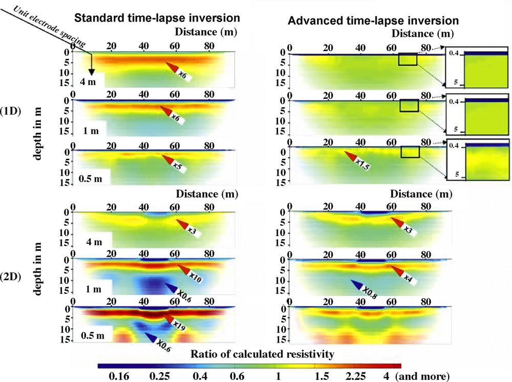
Result of time-lapse inversion of synthetic data sets (combined Wenner and dipole–dipole arrays). Ratio of calculated resistivity using standard and advanced inversion. Red arrows represent increases of resistivity, and blue arrows represent a decrease. The ratios of the calculated resistivity after infiltration to the initial calculated resistivity before infiltration are attached to the arrows.
Inversion en mode suivi temporel des jeux de données synthétiques (dispositifs Wenner et dipôle–dipôle combinés). Rapport des résistivités calculées en utilisant les modes d’inversion standard et amélioré. Les flèches rouges représentent des augmentations de résistivité calculée, les flèches bleues des diminutions. Le rapport de la résistivité calculée après l’infiltration sur la résistivité calculée initiale avant l’infiltration est indiqué à côté des flèches.
3.1 Synthetic models
3.1.1 1-D case
In the area between 0 and 0.4 m (thickness of the simulated infiltration), the ratio of calculated resistivity ranges between 0.6 and 0.8 for a standard inversion, for a unit electrode spacing of 4 m. For unit electrode spacing of 1 m, it ranges from 0.2 to 0.6, which is closer to the expected value of 0.1. Finally, with the smallest unit electrode spacing of 0.5 m, the ratio of the calculated resistivity is between 0.1 and 0.3, close to the required theoretical value. Using advanced inversion, the ratio of calculated resistivity follows the same trend for all the spacings. A slight improvement was noted for 0.5 m spacing data: the ratio reaches the ideal value of 0.1.
In the area between 0.4 and 2.5 m, the actual resistivity does not change; consequently, the calculated ratio should be 1.0. With standard inversion, all unit electrode spacings show an increase of the calculated resistivity model, the ratios have values ranging between 1.2 and 6 (Fig. 2, 1-D red arrow). When the advanced inversion is used, a clear improvement is obvious: the ratio is limited to the range between 1 and 1.2 only.
In the area between 2.5 and 5.3 m (clayey layer), the actual resistivity does not change; consequently the calculated ratio should also be 1. With standard inversion, an increase of 1.1 to 2.5 between 2.5 and 3.5 m is still found. With spacing of 0.5 m and standard inversion, the variation is limited to a value of ratio ranging between 1.1 and 1.7. It remains between 1 and 1.3 with advanced inversion. Deeper, between 3.5 and 5.3 m, the ratio of calculated resistivity is close to the expected value of one whatever standard or advanced inversion is used. In conclusion, it seems that the depth interval affected by resistivity artefacts is reduced with smaller unit electrode spacing.
Below 5.3 m in the sandy substratum, with a standard inversion, the resistivity decreases (ratio between 0.7 and 1 for all units of electrode spacing). With advanced inversion, the ratio remains between 0.9 and 1.1.
We drew two major conclusions. First, the resistivity variations at shallow depth and the infiltration depth are logically better resolved with shorter unit electrode spacing (0.5 m in our example). Second, the use of advanced time-lapse inversion with a decoupling line limits the resistivity artefacts. For example, the false increase of resistivity below the infiltration zone is limited to 1.3, while with standard inversion, it is greater than 5.
3.1.2 2-D case
- • From the surface down to 0.8 m at the centre of the model, the results are similar to the results obtained with the 1-D model. With standard inversion, the decrease of electrode spacing improves the delineation of the bulb. The ratio of calculated resistivity approaches the theoretical value of 0.1. Using advanced inversion and 4 m spacing, the bulb is poorly defined. The resistivity ratio lies between 0.5 and 0.24, quite far from the required value of 0.1. For unit electrode spacing of 1 and 0.5 m, the advanced inversion shows a homogeneous ratio with a value of less than 0.2.
- • In the zone 0.4 to 2.5 m, all spacings show that the ratio of the calculated resistivity model increases with both standard and advanced inversion as in the 1-D case. The calculated resistivity ratio reaches very high values (up to 19) with the standard inversion. For advanced inversion, the increase remains much smaller (around 4) with 1 m spacing.
- • Between 2.5 and 5.3 m, the calculated models are similar to what we obtained for the 1-D case.
- • For the substratum zone, the calculated variations are more noticeable. With both standard and advanced inversions and 4 m spacing, the ratio of the calculated resistivity model remains between 0.9 and 1.1, an acceptable result. With shorter spacing, the ratio of calculated resistivity varies between 0.5 and 0.8 for standard inversion, and between 0.8 and 1 for advanced inversion. However, even if the advanced inversion seems to give better results, the patterns of the resistivity ratio distribution appears complicated by the 2-D geometry of the infiltration. Some resistivity artefacts (increases) are visible in the lower left and right corners. They are considered to be boundary effects and are not analysed in this article.
The numerical modelling shows that at shallow depth, the ratio of calculated resistivity and the geometry of the infiltration are better resolved using the smallest unit electrode spacing. The false increase in the apparent resistivity during infiltration is reduced when the advanced inversion introducing a decoupling line is used. In the advanced approach, the calculated ratio is limited to 1.5 in 1-D (50%) and to 1.7 (70%) in 2-D, while with the standard approach, ratios of 2.5 (250%) or even 8 (800%) with 1 and 2-D cases are obtained, respectively.
At depth, the numerical modelling shows that the reduction of unit electrode spacing could generate several symmetrical zones on the cross-section with a decrease or increase of calculated resistivity. The contrast is greater in the 2-D case. Because we focused our work primarily on the removal of the most severe resistivity artefacts (increase of calculated resistivity) below the infiltration zone, the origin of smooth oscillations at depth is not investigated in this article. Effects of the regularization parameter, array used, or even data density might explain this phenomenon.
Finally, we showed that using the advanced time-lapse inversion, the calculated resistivity ratio is significantly closer to the resistivity model ratio, and is generally limited to ±0.2 (i.e. ±20% of resistivity variations).
3.2 Field data example
The field data set is a typical case showing resistivity artefact production after time-lapse inversion. This survey was not dedicated to shallow infiltration monitoring but rather to study recharge processes under an ephemeral gully in Burkina Faso, West Africa [5]. In regions with a low rainfall index and a monsoon climate, there is an increasing need for sustainable groundwater resources. This requires a better understanding of groundwater recharge zones. Recharge processes in semi-arid climates (rain < 600 mm) are mainly located below seasonal ponds [14,15], alluvial sandy fans [16] and intermittent (ephemeral) streams during monsoon events [7]. Quantification of infiltration rates and groundwater recharge relies generally on field measurements in boreholes by means of neutron probes, tensiometers, capacitive probes and piezometer networks. These point measurements need an optimized implementation with geophysical surveys.
The study area, in northern Burkina Faso, is a typical (1 ha) gully erosion area located at the outlet of an 82 ha catchment with a crystalline basement (Fig. 3). The surface conditions in the area are favourable to infiltration due to: (i) a fractured quartz vein; and (ii) sandy or pebble surfaces. Taking advantage of a long dry season followed by a short rainy one, we used the time-lapse ERT approach to carry out electrical resistivity monitoring during the rainy season, between June and September. We used two apparent resistivity data sets obtained just before (June) and just after the rainy season (September) to obtain a significant infiltration phenomenon. The stainless steel electrodes were left in the soil for the duration of the experiment. The cables were laid out each time.
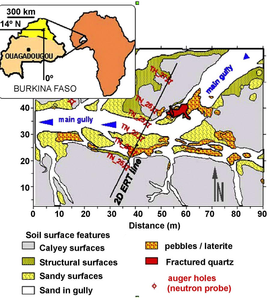
Location of the experimental site, geophysical survey and neutron probe measurements.
Localisation du site expérimental, des mesures géophysiques et des tubes d’accès de sonde à neutron.
To monitor expected infiltration down to depths of 5 m or more, we laid out a Wenner array profile along a line crossing the gully. A first acquisition was made with 1 m spacing along the entire length of the profile. The data set with 2 m was extracted from the 1 m data set for demonstration purposes in this paper. Then, three panels of apparent resistivity with the 0.5 m spacing data set were acquired by a classical roll-along technique, with three successive acquisitions involving 64 electrodes each. The data with 1 m spacing were added at depth to the 0.5 m panels. This avoids inversion distortions due to the lack of data at depth.
Measurements were made before noon to avoid high temperature variations. In addition, apparent resistivity variations were also monitored with time on a test site during the day to evaluate the effect of temperature on resistivity variations. We found that the apparent resistivity for short spacing (< 1 m) varied by less than 5% in the morning thus keeping temperature effects at an acceptable level. The infiltration pattern was also monitored with neutron probe measurements in six auger holes shown in Fig. 3.
The results obtained with both standard and advanced inversions are presented in Fig. 4. We positioned the decoupling line at a constant depth of 0.25 m corresponding to the average value given by the infiltration front derived from neutron probe measurements.
- • At shallow depth between 0 and 0.4 m, with a large unit electrode spacing of 2 m, the ratios of calculated resistivity are 1.3 and 4 using standard and advanced options respectively, indicating that the infiltration is not visible. For smaller spacing (1 m) the infiltration is still not detected with the standard inversion. With advanced inversion, the infiltration is clearly seen with a ratio below 0.5 and 1.With the smallest spacing of 0.5 m, the ratio of resistivity is lower than 0.5 whatever type of inversion is used;
- • between 0.5 and 3 m, for all spacings, the standard inversion shows a calculated resistivity ratio, which ranges between 1.2 and 5. When advanced inversion is used, the increase is limited to a ratio ranging between 1 and 1.5;
- • below 3 m, for all inversion and with a unit-electrode spacing of 2 m, the ratio of resistivity remains between 0.9 and 1.2. With unit electrode spacing of 1 m, the ratio of calculated resistivity is in the range of 1–1.3 for standard and advanced inversion. For a spacing of 0.5 m, results show noticeable variations between 1 and 1.3 marked by a red arrow in Fig. 4. At the right of the cross-section below the position of 44 m, the ratio of calculated resistivity ranges between 0.5 and 0.8 as shown by a blue arrow.
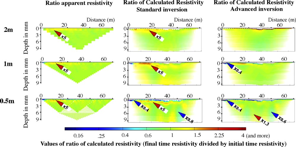
Standard inversion and advanced inversion results for field data with three different unit electrode spacings (2, 1 and 0.5 m).
Résultats des inversions en mode standard et amélioré pour le jeu de données de terrain, avec trois écartements unitaires d’électrodes (2, 1 et 0,5 m).
4 Discussion
4.1 Comparison with neutron probe data
Fig. 5 presents the comparison between standard and advanced time-lapse inversion of ERT with the smaller electrode spacing (0.5 m) versus neutron probe data. The infiltration front is drawn according to the measurements of the six neutron tubes (TN 22, 23, 24, 25, 26 and 27). Only TN 23, 24, 25 and 26 are shown for clarity. All tubes show infiltration down to less than 0.4 m except TN24 where the infiltration deepens to 0.80 m. In addition, below TN24, a very localized water invasion was recorded at a depth of 4 m during the rainy season. We attribute this phenomenon to a local lateral invasion due to the proximity of the fractured quartz vein. Five major conclusions were drawn from the comparison of neutron probe data and ERT:
- • first, for the standard time-lapse inversion, we note that if we draw the contour line of ratio 0.8 near the surface, the shape of this line is in agreement with the neutron probe variation;
- • second, the increase of calculated resistivity just below the infiltration was not corroborated by neutron probe measurements as expected from our numerical modelling. We confirm here the resistivity artefact creation using standard inversion. In the deeper part of the section, the variations of the ratio are high (range 1 to 1.7);
- • third, for the advanced inversion using a constant thickness of decoupling (0.25 m), the decrease of calculated resistivity is strictly limited inside the decoupling zone;
- • fourth, the increase of calculated resistivity below the infiltration is clearly reduced, not only with the reduction of the area involved, but the ratio also remains limited to less than 2. In addition, in the deeper part of the section, the variations of the ratio are not only lower (range 0.9 to 1.1 with some local values reaching 1.3), but affect a smaller area of the section;
- • fifth, the water invasion noted for tube TN24 at 4 m depth is noticed by both inversions. It is, however, comparable to other variations calculated laterally at the same depth. These variations are not corroborated by neutron probe data. They could also be the result of geometrical oscillations in the inversion, as already noted at depth with our numerical modelling of a 2-D infiltration object.
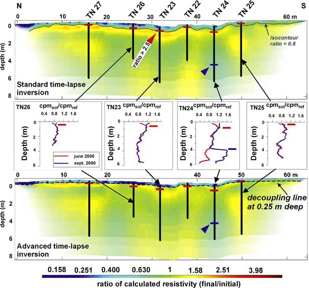
Comparison of neutron probe data with standard (top) or advanced (bottom) time-lapse inversions. For standard inversion, the contour line of 0.8 is marked by a continuous grey line to show the good accordance with neutron probe data (the infiltration front is shown by short red lines). For advanced inversion, the position of the decoupling line is marked by a black dotted line. The blue arrow shows the localized water invasion at 4 m depth below neutron probe tube TN 24.
Comparaison des résultats obtenus avec la sonde à neutron et les inversions en mode de suivi temporel pour le mode standard (en haut) et amélioré (en bas). Pour le mode standard, la ligne d’isocontour de rapport 0,8 est marquée avec une ligne grise continue, pour montrer la bonne correspondance avec les données de sonde à neutron (le front d’infiltration est montré avec de courts traits horizontaux rouges). Pour le mode d’inversion amélioré, la position de la ligne de découplage est marquée par une ligne noire pointillée. La flèche bleue montre une invasion d’eau très localisée à 4 m en dessous du tube neutronique TN24.
Finally, we noted that using standard inversion, severe resistivity artefacts of increasing resistivity were produced below the infiltration front, as predicted by the numerical modelling. The only benefit obtained from the standard inversion is that the irregular shape of the infiltration front fits the neutron probe data. With the advanced inversion, we noted a clear improvement in resistivity artefact removal. We used a constant thickness of decoupling line. Zones with an increase in calculated resistivity at depth are still present, but within a smaller variation range. This is not entirely satisfactory. We investigated further in the decoupling.
4.2 Influence of the geometry of the decoupling line
Considering that the infiltration geometry could not be well known in the field due to a lack of boreholes or other methods, we investigated the effect of three different geometries of the decoupling line. The results are presented in Fig. 6. Three cases are discussed: (i) no knowledge of the depth of the infiltration front (decoupling line at a constant depth all along the ERT profile); (ii) a precise but punctual knowledge of the depth of the infiltration front; (iii) a complete knowledge of the depth of the infiltration front.
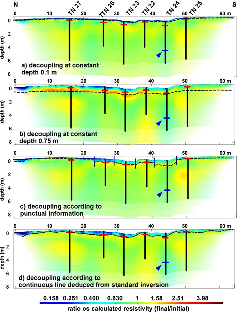
Effect of the geometry of the decoupling line. (a) and (b). Decoupling line with a constant depth of 0.1 and 0.75 m, respectively. (c). Decoupling line using information obtained with neutron probe data. (d). Decoupling line with irregular shape deduced from contour line of ratio 0.8 obtained with standard time-lapse inversion with smallest unit-electrode spacing of 0.5 m (see Fig. 4).
Effet de la géométrie de la ligne de découplage. (a) et (b). Lignes de découplage placées à 0,1 et 0,75 m de profondeur respectivement. (c). Ligne de découplage placée selon l’information obtenue avec les tubes neutroniques. (d). Ligne de découplage avec une forme irrégulière déduite de l’isocontour de rapport 0,8, obtenu avec le mode d’inversion standard et le plus petit écartement d’électrodes de 0.5 m (voir Fig. 4).
The first case corresponds to the one where the interpreter gives only an estimate of the thickness of the infiltration front as we did when interpreting our field data. As shown in Fig. 6a, and b, for two different decoupling depths, the time-lapse ERT gave different results: for a decoupling depth of 0.1 m, the increase of calculated resistivity remains acceptable and lower than 1.25 just below the infiltration. This result is comparable, or slightly better, than what we obtained with a decoupling depth of 0.25 m (as shown also in Fig. 4). Using a much higher infiltration depth as decoupling line, for example 0.75 m (Fig. 6b), ERT time-lapse inversion no longer fits the neutron probe data. ERT exhibits a significant increase of resistivity (ratio of more than 3) at the north of the section for example, not corroborated by neutron probe data.
The second case corresponds to a precise but punctual knowledge of the depth of the infiltration front. We introduced six decoupling lines at six constant depths indicated by the six neutron probe data. Each line is centred with respect to the tube, its length is arbitrarily limited laterally to the mid point between two tubes. The results shown in Fig. 6c exhibit promising improvements in resistivity artefact removal, especially in the northern part. However, at the centre of the gully, an increase of calculated resistivity is magnified.
The third case considers a complete knowledge of the infiltration front as a continuous line. This information could be extracted from other data in the field (dense TDR measurements or ground penetrating radar profiling). For our study, we took advantage of the good agreement noted between the shape of the ERT contour line produced with the standard time-lapse inversion and the neutron probe. We thus generated a decoupling line that respects exactly the shape of the calculated contour line. By comparison with neutron probe data, we choose the contour line of 0.8. The results are shown in Fig. 6d. A general improvement is noted. The increase of the calculated resistivity is significantly reduced or even removed just below the infiltration front. The oscillations of the resistivity ratio at depth are still present but their amplitude stays within a limited range (between 0.85 and 1.25). The decrease of the calculated resistivity at 4 m depth below the neutron tube TN 24 appears magnified (slight decrease of the ratio).
We demonstrate here that the position and the geometry of the decoupling line are of great importance. Acceptable results are obtained with our field data using a small thickness of decoupling (0.1 m). In addition, and for other surveys, the approach considering a continuous knowledge of the depth of the infiltration front is by far the best, even if some resistivity artefacts are still present but limited to a range between 0.85 and 1.25. Then one can use the shape of the infiltration given by standard time-lapse inversion as the decoupling geometry, but it is in any case essential to have external data at some points along the profile. Moreover, small unit electrode spacings are required during data acquisition. For further studies, additional improvements could be made in time-lapse inversion by using other a priori information such as invariant zones (for example the knowledge of the groundwater conductivity with time). This approach has already been tried by Vesnaver et al. [23] for seismic inversion and by Nguyen and Kemna [18] for ERT inversion, but it was not tested in this study, because the field data did not allow us to fix an invariant zone at depth.
4.3 Discrimination between resistivity artefact and true hydrological processes
We examine here the capacity of the advanced interpretation to discriminate between a resistivity artefact and a true hydrological process. We chose a common but important case for soil and agronomical sciences: the characterisation of the zone where the plants are taking up water within the root zone and where resistivity is likely to increase. Therefore, as we have seen from the modelling and field data, the resistivity artefact of increasing resistivity at intermediate depth might be wrongly interpreted as a drying zone (root-zone). Finally, the question arises: if a true drying zone exists below the infiltration in the same place as resistivity artefacts, what is the efficiency of the advanced inversion? Does it display correctly the true phenomenon of an increasing resistivity? A scenario that includes a shallow infiltration and a drying zone below was simulated using the 2D model presented in Fig. 1. Fig. 7 presents the model that includes the drying zone and the results obtained with standard and advanced inversions. The standard inversion displays a strong increase of resistivity, ratio more than 8, between 2 and 5 m, and a strong decrease below (ratio less than 0.4). When one looks at the advanced inversion, the increase of resistivity below the infiltration is also seen and its value (ratio near 2.5) agrees well with the expected value of 2. Below, the variation of resistivity remains within the range 0.7 to 1. As a conclusion, if a true increase of resistivity is present in the soil at intermediate depth, it can be identified and correctly quantified by the advanced time-lapse inversion. Using standard inversion, unreliable values are obtained as resistivity artefact and the true phenomenon add their effects.
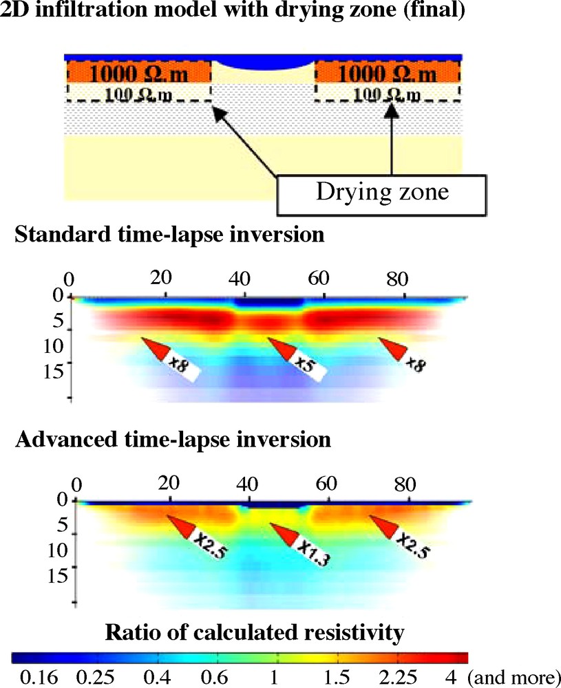
Comparison between standard and advanced time-lapse inversion using a scenario with a drying zone below the infiltration as shown on the model. The true increase of resistivity is 2 and it is satisfactorily reconstructed with advanced inversion using a decoupling line (below).
Comparaison entre les modes d’inversion en suivi temporel standard et amélioré en utilisant un scénario de dessèchement, dans une zone située juste au-dessous du front d’infiltration, comme le montre le modèle synthétique (en haut de l’image). La véritable augmentation de résistivité d’un facteur 2 est reconstruite de façon satisfaisante, avec le mode d’inversion amélioré qui utilise une ligne de découplage (en bas de l’image).
5 Conclusion
Time-lapse ERT inversion can produce resistivity artefacts in certain circumstances already pointed out in previous studies. For example, when the actual resistivity decreases at shallow depth, a typical resistivity artefact is an increase of calculated resistivity at intermediate depths, whereas the actual resistivity does not change. Therefore, results of time-lapse ERT could lead to false interpretations and ERT may not be reliable for studying changes in resistivity at depth. We investigated the effect of a shallow variation of resistivity within the first decimetres of the soil on time-lapse ERT inversion using numerical modelling to show a typical ERT resistivity artefact. We show that 2-D infiltration geometry enhances the resistivity artefact production by creating additional oscillations of calculated resistivity variation at depth. We used an advanced time-lapse inversion introducing a shallow decoupling line as a priori information corresponding to a constant thickness of the infiltration front, supposed to be known from external data. Using this advanced inversion, the resistivity artefact production is significantly reduced. The wrong increase of calculated resistivity is limited to a ratio of less than 1.3 whereas it grows to 3 or even more when standard time-lapse inversion is used.
The advanced time-lapse inversion was tested on field data and the results corroborate the conclusions derived from the numerical modelling:
- • data sets using short unit-electrode spacing are required to provide a convenient base for time-lapse ERT in case shallow infiltration (or evaporation) is present;
- • using a standard (non-decoupling) approach, the resistivity artefact creation (i.e. increase of calculated resistivity at intermediate depth) is confirmed;
- • using standard inversion, the infiltration front can be delineated if short electrode spacing is used. In this case, a comparison with neutron probe data is necessary to identify the correct calculated resistivity isocontour and thus delineate the position of the infiltration front in the ERT image. Then, the infiltration front positioned with ERT can be used for advanced inversion;
- • when advanced inversion that incorporates a decoupling line of constant thickness at shallow depth is used, the resistivity artefacts noted at intermediate depth are significantly reduced. We increased the resistivity artefact reduction by using a continuous line of variable thickness. The position of this line was deduced from the comparison between neutron probe data and standard inversion data. This allowed us to remove almost completely the resistivity artefact of increasing resistivity at intermediate depths. However, some oscillations at depth within a range of ratio 0.8 to 1.2 (i.e. ±20%) are still present and could be smoothed by tuning other inversion parameters such as regularisation factors.
Finally, when performing time-lapse ERT surveys in the presence of shallow infiltration or evaporation, we advocate measuring dense apparent resistivity data at shallow depth using small unit-electrode spacing (or shallow electromagnetic profiling). Even with short electrode spacing, a standard time-lapse inversion may exhibit false resistivity variations below the infiltration or evaporation front. To remove those unwanted resistivity artefacts, we need to incorporate a shallow continuous decoupling line into the inversion. In case of infiltration, this decoupling line is the infiltration front. The position and the shape of this line need to be defined and controlled with external information such as neutron probe data (or any other method available) as well as deduced from the ERT survey itself. With this approach, more reliable time-lapse ERT results are obtained, not only for shallow depths, but also on deeper changes in resistivity in the pseudo-section, leading to a better characterization of hydrological processes.
Acknowledgments
We wish to thank French EC2CO project ONDINE for funding part of this research. The INERA Institute in Burkina Faso provided access to the experimental site. Yann Le Troquer and Burkinabese staff are warmly thanked for field data acquisition. We are very grateful to Dr Thomas Ingeman-Nielsen for his helpful comments on the first version of the manuscript.