

1 Introduction
Solute migration in aquifers is one of the most debated issues in hydrogeology, since most experimental results display large deviations from the standard asymptotic Fickian dispersion theories. Indeed, an increasing number of tracer tests [1,2,18,22,29] shows that anomalous dispersion is the rule rather than the exception in natural geologic formations, and it becomes therefore more and more certain that Fickian models fail to capture the real nature of the dispersion in natural systems submitted to common hydrological stresses. The key issue to identify non-Fickian solute transport from a tracer test breakthrough curve (BTC, i.e. concentration measured at a given observation point) is the occurrence of long-tail late-time arrivals compared to the Fickian solution (Fig. 1). Usually, the BTC tail appears to decrease more or less as a power-law of time

Example of BTC normalized by C0 × Tinj (so that it integrates to 1) measured at the Ses Sitjoles test site showing the power law asymptotic behaviour C(t)∼t−α at large elapsed time. The dotted curve is the best fit obtained using the standard Fickian dispersion model.
Exemple de courbe de restitution normalisée par C0 × Tinj (de manière à ce qu’elle intègre à 1), mesurée sur le site expérimental de Ses Sitjoles, montrant le comportement C(t)∼t−α pour les grandes valeurs du temps après injection. La courbe en pointillé représente le meilleur calage obtenu en utilisant le modèle standard de dispersion Fickienne.
Anomalous dispersion arises from the heterogeneity of flow fields caused by the heterogeneity and the spatial correlation of the permeability structures. Often, spatially correlated heterogeneities extend over several spatial scales in geological media and hierarchical flow path models displaying broader distributions of velocities are natural candidates to explain non-Fickian transport [e.g. 3, 11, 12, 24]. The stratified model, in which the overall mass transport is the sum of elementary transports in independent channels of distinctly different properties (leading to different flow rates and residence times), is the end-member model with infinitely correlated velocities [2,16]. In this case, the distribution of channel properties will control the shape of the power-law decaying BTC. Conversely, anomalous dispersion due to highly heterogeneous flow fields can be accounted for in the framework of Continuous Time Random Walks (CTRW) [10]. The CTRW model assumes that the continuous movement of a solute particle in a given velocity field is modelled by discrete jumps of a random walker. The length of the jump and the waiting time between two successive jumps are drawn from a stationary time-space joint probability density function ψ(x,t) reflecting the medium heterogeneity [4]. In general, it is admitted that the jump length and the waiting time are independent variables for solute transport in porous media, and furthermore, it is assumed that ψ(x,t) can be modelled by a power law distribution
Conversely, non-Fickian transport is widely observed at laboratory scale even in porous media thought as macroscopically homogeneous [e.g. 7, 25]. Consequently, as non-Fickian transport is observed at virtually all scales, it is worth considering mass transfer into small-scale geological structures where diffusion dominates as another possible origin of anomalous dispersion. For instance, the mobile-immobile multirate mass transfer (MIM) model assumes mass exchanges between the moving fluid and a less permeable domain in which the fluid is considered as immobile [6,8,15,17,31]. Here, non-Fickian transport is not controlled by the characteristics of the flow field, but by the diffusion-controlled transport of the solute particles in dead-end structures. The late-time BTC concentration C(t) is proportional to the time derivative (noted
| (1) |
From the above discussion, it comes out that both water velocity heterogeneity controlled by large-scale structures and diffusion processes controlled by small-scale structures lead to anomalous transport and similar power-law decaying BTCs. Furthermore, they are both equivalently modelled by CTRW using a power law decaying distribution of the waiting time, for instance. However, the discrimination between the control of the large-scale heterogeneity of the permeability field and that of the small-scale diffusion-controlled structures is a critical issue for model parameterisation and upscaling. Yet, it is a difficult task because it is most probable that both may be present simultaneously in several heterogeneous reservoirs. Nevertheless, it is possible of minimizing the velocity spatial correlation using Single-Well Injection-Withdrawal (SWIW) tracer tests and by selecting reservoir targets displaying large-scale homogeneity.
SWIW tracer tests, also called push-pull tracer tests, consist in injecting a given mass of tracer in the medium and reversing the flow after a certain time in order to measure the tracer breakthrough curve at the injection point [13,19,33]. This technique presents several advantages. First, the reversal of flow warrants an optimal tracer mass recovery, which is of importance to produce quantitative results. Second, the SWIW tracer test allows measuring the irreversible dispersion (or mixing) whereas the reversible dispersion (i.e., the spreading induced by a long-range correlated path) taking place during the tracer push phase is cancelled during the withdrawal phase [2,21]. The quantification of the reversible and irreversible dispersion refers to a given scale of observation which, in our case, is the maximal distance migrated by the tracer during the SWIW tracer test. More precisely, velocity correlation, over distances smaller than the exploration size, will result in irreversible dispersion (diffusion and mixing) whereas advection spreading due to velocity correlation larger than the exploration size will be cancelled (see Fig. 1 in [14]). Thus, the dispersion measured using SWIW tests is only caused by tracer molecules that do not follow the same path in the injection and the withdrawal phases. In this case, the observation of non-Fickian transport may indicate the occurrence of mass transfers into immobile zones. Third, using SWIW tests, the tracer may be pushed at different distances from the injection point, thus visiting different volumes of the system using a single well. This allows investigating the dispersion processes for increasing volumes of reservoir [23], studying the scale effect on dispersion, and subsequently testing the different assumptions concerning the origin of the anomalous dispersion (i.e. scale-dependent flow velocity heterogeneity versus pore scale diffusion models).
In theory, all the information required to characterize the anomalous dispersion can be retrieved from the BTC shape and specifically from the BTC tailing. However, in practice, it is generally difficult to evaluate whether the observed BTC tail represents the rate-limited behaviour only or a transitional behaviour in the vicinity of the main concentration peak, unless concentration is measured for long times after the advection peak has passed. Therefore, long-lasting recording of the tracer recovery and high-resolution sensors are required. In practice, the concentration must be measured over several orders of magnitude (4 to 5 generally).
The aim of this article is to present new equipment recently developed to investigate (anomalous) dispersion from laboratory to field scale. First, we will focus on pointing out the capacity of the fluorescent sensor TELog to produce unmatched in situ high resolution fluorescent dyes concentration monitoring. Second, we will describe the downhole probe CoFIS that is designed to perform fully controlled, long-lasting SWIW tracer tests. Finally, some examples of results of tracer tests in fractured and porous media are presented.
2 Equipment and methodology
2.1 Fluorescent dye measurement using the TELog tool
For measuring dispersion of a passive tracer, it is essential to use low concentrations of tracer in order to avoid density effects [32], while ensuring that the tracer concentration can be measured over four orders of magnitude, at least. A specific high-resolution sensor, called TELog, was developed to account for these requirements. In TELog, uranine and sulforhodamin fluorescent dyes and turbidity are measured using a set of short-range band-pass (interference) filters (Fig. 2c) and a high-sensibility photomultiplier with a computer-assisted adjustable gain system (Fig. 3). The use of a motorized cylinder containing the band-pass filters allows switching from one optical path to another in order to recurrently measure the two fluorescence signals, the turbidity and the excitation LEDs intensity. In standard mode, an average value (and its standard deviation) over 30 samples is recorded every 9 sec together with a similar average of the dark signal (i.e., the noise of the photomultiplier), which was proven to be always lower than a few ppt (1 ppt = 10−12 g/g). The TELog probe is built around a microcontroller (Texas Instruments MSC1211) with built-in precision Analog-to-Digital (ADC) and Digital-to-Analog Converters (DACs). The microcontroller uses one DAC to power the potentiometer that measures the position of the cylinder, two DACs power the external and internal pressure sensors and one DAC drives the gain of the PMT (high voltage control). Every measurement is time-stamped by means of the Real Time Clock, written in the flash memory and sent to the surface through the RS485 driver. It is possible to use the TELog as a standalone probe from a computer or connected to the CoFIS probe. Different modes are available, slow or fast measurement (i.e. with no sample averaging) and combination of measurements.
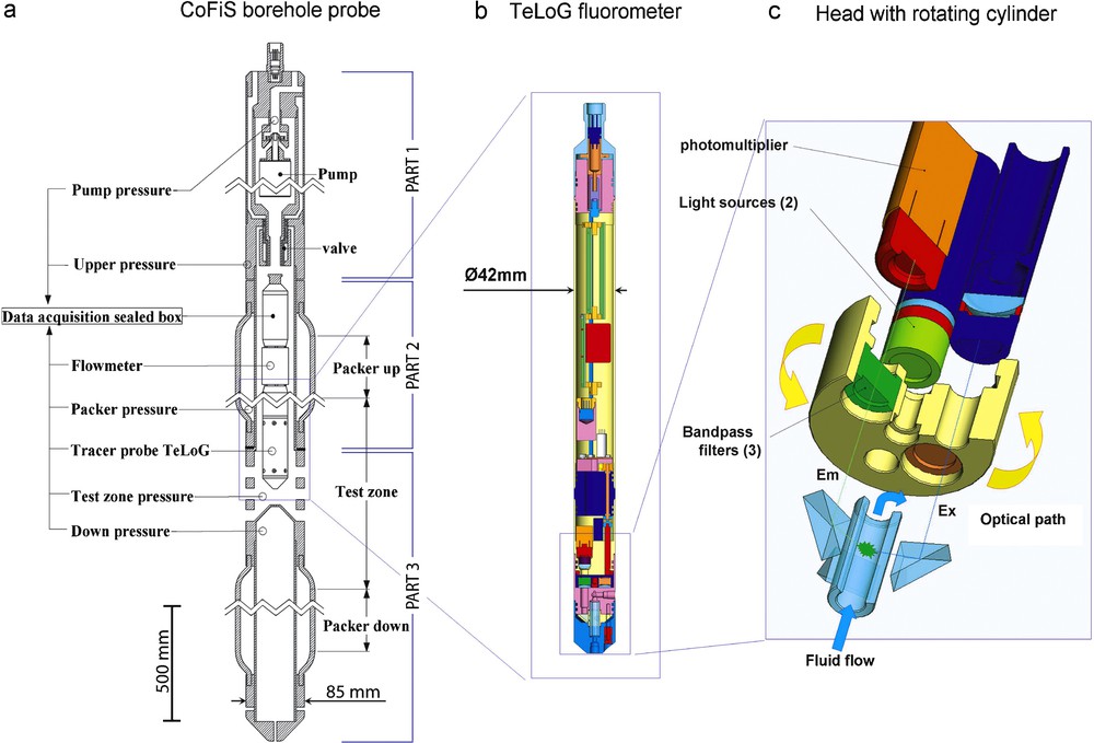
a: Schematic representation of the CoFIS probe (the horizontal scale is exaggerated for better visualization); b: Schematic representation of the TELog sensor that is installed in the CoFIS probe for fluorescent dye measurement; c: details of the TELog measurement head displaying the optical path. The recurrent measurement of two different fluorescent tracers (e.g. uranine and sulforhodamine) and water turbidity is performed by computer-controlled rotation of the band-pass filter holder, while activating one of the two pulsed-led light sources. Uranine signal is measured with a 485 ± 10 nm excitation filter and a 530 ± 12 nm emission filter, sulforhodamine signal is measured with a 530 ± 12 nm excitation filter and a 590 ± 17 nm emission filter, turbidity is measured at 530 ± 12 nm and LEDs intensity is measured using a light-guide bypassing the measurement chamber. Masquer
a: Schematic representation of the CoFIS probe (the horizontal scale is exaggerated for better visualization); b: Schematic representation of the TELog sensor that is installed in the CoFIS probe for fluorescent dye measurement; c: details of the TELog measurement head ... Lire la suite
a : représentation schématique de la sonde CoFIS (l’échelle horizontale est exagérée pour une meilleure visualisation des éléments) ; b : représentation schématique de la sonde TELog qui est installée dans la sonde CoFIS pour mesurer la concentration en traceurs fluorescents ; c : détails du système optique de la sonde TELog. La mesure récurrente de deux traceurs (ex : uranine et sulforhodamine) et de la turbidité est réalisée par la rotation, contrôlée par microprocesseurs, du barillet où sont installés les filtres et des deux LED pulsées qui fournissent la lumière. Le signal de l’uranine est mesuré avec un filtre d’excitation à 485 ± 10 nm et un filtre d’émission à 530 ± 12 nm ; le signal de la sulforhodamine est mesuré avec un filtre d’excitation à 530 ± 12 nm et un filtre d’émission à 590 ± 17 nm; le signal de turbidité est mesuré à 530 ± 12 nm et l’intensité de chaque LED est mesuré grâce à un guide de lumière permettant de bipasser la zone de mesure du fluide. Masquer
a : représentation schématique de la sonde CoFIS (l’échelle horizontale est exagérée pour une meilleure visualisation des éléments) ; b : représentation schématique de la sonde TELog qui est installée dans la sonde CoFIS pour mesurer la concentration en traceurs fluorescents ; c : détails ... Lire la suite
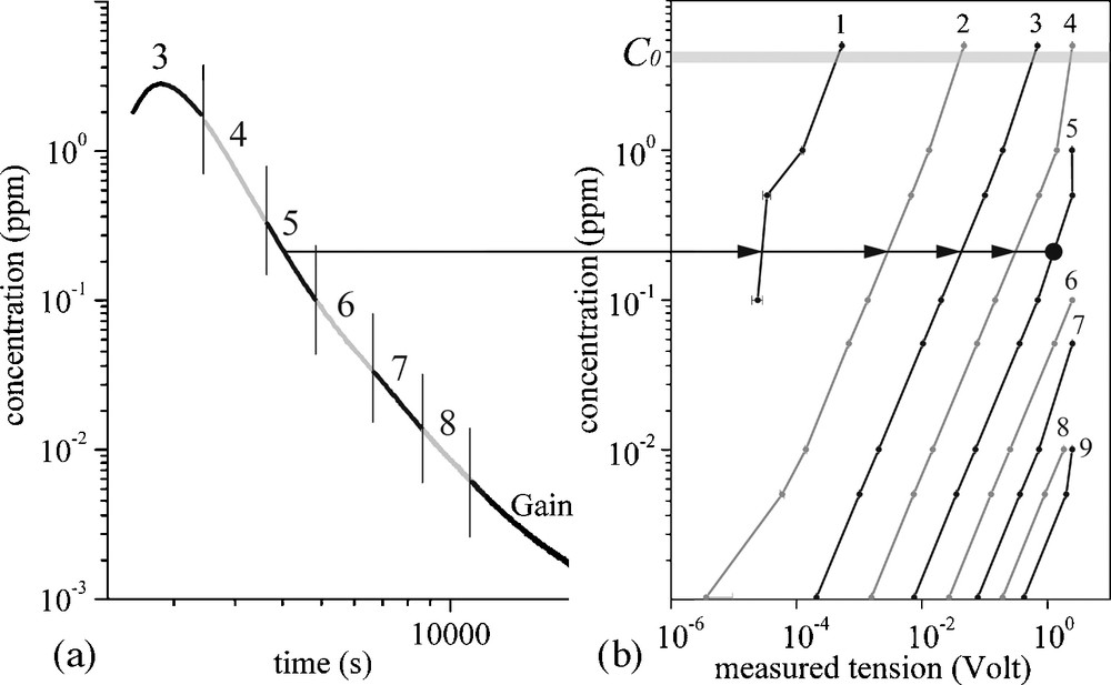
(a): Example of a raw BTC. The use of self-adaptive gain allows optimizing the signal-to-noise ratio over more than five orders of magnitude from about 100 ppt to 500 ppm. In this figure, gains from 3 to 9 are reported. For each gain, raw data range from 0 to 5 Volts with a theoretical resolution of 6 × 10⁻⁷ Volts (23 bits) and a measured accuracy of about 3 × 10⁻⁵ Volts (∼ 17 bits); (b): Calibration curves for the different values of the gain (1 to 9); gains are scanned from low value (1) to the highest value corresponding to the best signal-to-noise ratio (higher voltage) in order to avoid overlighting of the photomultiplier. Masquer
(a): Example of a raw BTC. The use of self-adaptive gain allows optimizing the signal-to-noise ratio over more than five orders of magnitude from about 100 ppt to 500 ppm. In this figure, gains from 3 to 9 are reported. For each ... Lire la suite
(a) : exemple de courbe de restitution mesurée par le capteur TELog. L’utilisation d’un système de gain auto-adaptatif permet d’optimiser le rapport signal-sur-bruit sur plus de cinq ordres de grandeur, de 100 ppt à 500 ppm. Dans la figure, les gains de 3 à 9 sont utilisés dans cet exemple. Pour chacun des gains, les valeurs sont comprises entre 0 et 5 Volts, avec une résolution théorique de 6 × 10⁻⁷ Volts (23 bits) et une précision de mesure de 3 × 10⁻⁵ Volts (∼ 17 bits) ; (b) : courbes de calibration pour les différentes valeurs de gain (1 à 9). Les gains sont testés successivement du gain le plus faible (gain 1) vers le gain le plus fort (gain 9), jusqu’à ce que la mesure correspondant au meilleur rapport signal-sur-bruit soit atteinte (voltage le plus fort), afin de ne pas éblouir le photomultiplicateur. Masquer
(a) : exemple de courbe de restitution mesurée par le capteur TELog. L’utilisation d’un système de gain auto-adaptatif permet d’optimiser le rapport signal-sur-bruit sur plus de cinq ordres de grandeur, de 100 ppt à 500 ppm. Dans la figure, les gains de 3 ... Lire la suite
Pre- and post-experiment calibrations were performed, showing that reproducibility is better than a few tens of ppt without any further correction. Fig. 3b displays the calibration curves as measured in the laboratory using a set of reference solutions for which the dilution procedure was controlled a posteriori by spectrometry measurement using a SHIMADZU RF 5301PC spectrofluorometer. An example of recovery curve displaying the calibrated response for each gain is given in Fig. 3a, where we can observe that the concentration curve is perfectly continuous over the whole range of measurements. Processing the raw data is quite simple once we have the gain-dependent calibration matrix, because the tracer concentration depends linearly on the measured dye concentration (Fig. 3b). Tracer concentration is given by the relation:
2.2 SWIW tracer test using the CoFIS probe
A SWIW tracer test consists in injecting a tracer pulse (duration Tinj), flushing it with water (duration Tpush), and then pumping it back at the same flow rate until the tracer concentration falls below the sensor resolution. The SWIW tracer test methodology using the CoFIS probe is presented in Fig. 4.
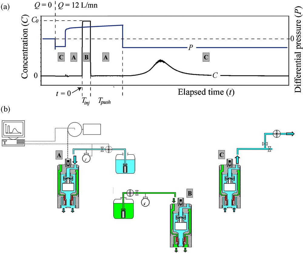
(a): Example of SWIW tracer test monitoring. Tracer concentration and pressure are reported versus time; (b): Schematic representation of the flow circuit in the CoFIS probe which is determined by the position of the remote-controlled solenoid slide-valve.
(a) : exemple montrant la procédure de réalisation d’un traçage écho. La concentration en traceur et la pression sont reportées en fonction du temps ; (b) : représentation schématique du trajet du fluide dans la sonde CoFIS, qui est déterminé par la position de l’électrovanne contrôlée depuis la surface.
The CoFIS probe (8 m long and weighting 110 kg) is transported in three parts that are assembled vertically atop the hole entry (Fig. 2a). The installation of the CoFIS probe downhole (e.g. at 100 m depth) can be completed by three persons in about 6 hours. The probe is hanged by a logging-standard 3/16 inch cable (operated by a Robertson Geologging winch) containing four electrical cores used to power the acquisition electronics (two cores) and the sensors and transmit the data to the surface panel (two cores).
The probe is also connected to the surface by the water and tracer hoses, the downhole pumps (three pumps) power wire and the packer inflation hose (Fig. 5). The hoses and the power wire are hold tightly to the logging cable every 25 m using screwed clampers.
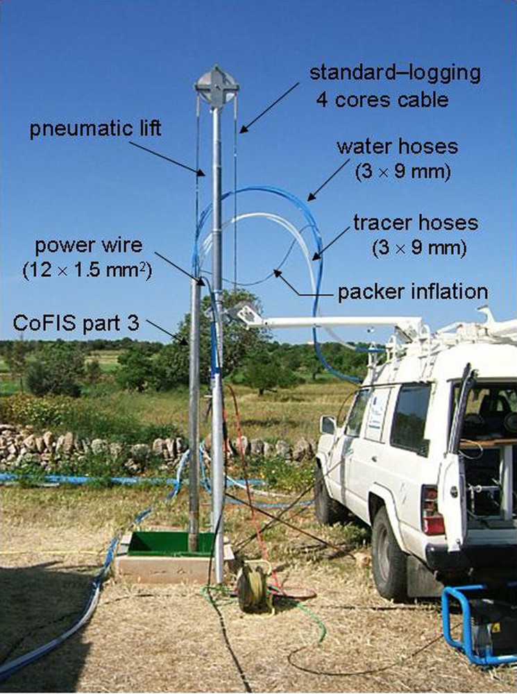
The CoFIS probe ready to be down-lifted into a 4.5-inch diameter unscreened borehole at the Ses Sisjoles test site. The probe is operated in the hole using a powered winch installed in the truck, while the pneumatic lift is used for the assembling of the three parts of the probe.
Photo de la sonde CoFIS prête à être descendue dans un forage non tubé de 114 mm de diamètre sur le site de Ses Sisjoles. La sonde est déplacée dans le forage grâce à un treuil installé dans le véhicule. Le bipode équipé d’un vérin pneumatique est utilisé pour assembler les trois parties de la sonde au-dessus du forage.
In the CoFIS probe, the injection zone of 0.675 m in length is delimited by a dual-packer system. Packers are 2.5 m long for an optimal sealing of the measurement zone during long-lasting SWIW tracer tests. The probe is designed to avoid immobile zones in the circuit and minimize the volume of the pumping chamber in order to reduce mixing in the system. This volume is less than five litres including the annulus between the tool and the well wall. Pressure sensors are fitted above the upper packer, below the lower packer and in the pumping chamber, which is equipped for receiving specific measurement probes such as the TELog instrument. Conversely, others sensors can be easily fitted. For instance, we used a IDRONAUT OCEAN-SEVEN 304 probe for performing tracer tests using water salinity measurements at the Ses Sitjoles test site (Mallorca, Spain, see section 3.2), but in this case, the tracer concentration is measured over two orders of magnitude only, and the asymptotic behaviour of the BTCs was incompletely assessed (Fig. 7).

Normalized BTCs (log-log plot) measured at the Ses Sitjoles test site well MC2 depth 94 m, for different values of Tpush. Black curves are measured using the TELog sensor. The grey curve partially overlapping the curve for Tpush = 40 min is the BTC obtained using the conductivity measurement (Cw). Note that in this case, the BTC slope value could have been misevaluated.
Courbes de restitution normalisées par C0 × Tinj (représentation log-log), mesurées sur le site expérimental de Ses Sitjoles dans le puits MC2, à la profondeur de 94 m, pour différentes valeurs de Tpush. Les courbes en noir représentent les courbes de restitution mesurées avec le capteur TELog. La courbe en gris qui se superpose partiellement à la courbe pour Tpush = 40 minutes est la courbe de restitution obtenue en utilisant un capteur de conductivité (Cw). On notera que la mesure de Cw n’aurait pas permis d’évaluer correctement la pente asymptotique de la courbe de restitution. Masquer
Courbes de restitution normalisées par C0 × Tinj (représentation log-log), mesurées sur le site expérimental de Ses Sitjoles dans le puits MC2, à la profondeur de 94 m, pour différentes valeurs de Tpush. Les courbes en noir représentent les courbes ... Lire la suite
Data streams coming from TELog (e.g. concentration) and CoFIS (e.g. pressure) are multiplexed downhole. Digitalized data are transmitted to the surface via a standard logging four-core cable and then multiplexed with the surface parameters, i.e. the flow rate and the pressure of the tracer injection hydraulic line, of the flushing water injection line and of the withdrawal line. Each of these hydraulic lines is equipped with a dedicated pumping system. The flow rate is controlled by tuning the pump engine rotation speed using a frequency generator. The withdrawal pump system is in the downhole probe CoFIS whereas the injection (tracer and flushing water) pumping system is at the ground surface. Details of the downhole and surface equipment are given in Fig. 4b. The switching from any of the lines (e.g. from tracer injection to water flushing injection) is operated downhole in the hydraulic chamber by a remote-controlled solenoid slide-valve. This system allows performing sharp rectangular pulse injections of duration (Tinj) as short as 120 sec.
3 Experimental results
3.1 SWIW tracer tests in a single fracture
CoFIS was first deployed at the Lavalette experimental site, which is located 3 km away from the Montpellier University campus (France). The test site comprises three unscreened wells of diameter 4.5 inches. The aquifer is a fractured marly limestone (age Valanginian) unconformly overlaid by Holocene deposits. A detailed description can be found in [30]. SWIW tracer tests have been performed at a depth of 60.5 m where a single sub-horizontal fracture was observed using optical and acoustic well-wall imaging. Pumping tests and flowmeter tests revealed that this fracture is hydraulically active and connected to a similar fracture pattern observed in the two other wells at distance of 5 and 10 m, respectively.
For these experiments, we used a solution of 2 ppm mass of a 99% pure uranine power diluted in the formation water previously extracted from the borehole. Fig. 6 displays some results for different Tpush durations at constant flow rate as well as for different flow rates at constant Tpush. The asymmetry of the BTCs is easily visible even when not using log-log representation, emphasizing a highly non-Fickian response. As expected for SWIW tests, the maximum concentration (Cmax) and the time at which the maximum concentration occurs do not depend on the value of the injection/withdrawal flow rate Q.
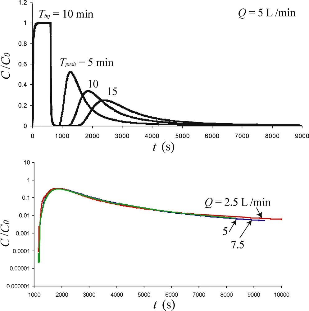
BTCs normalized by C0 measured at the Lavalette test site (single sub-horizontal fracture) for Tinj = 10 min. Top: results for Tpush = 5, 10 and 15 min with Q = 5 L.min−1 displaying dissymmetrical BTCs. Bottom: results for Tpush = 10 min for 2.5 < Q < 7.5 L.min−1 (semilog plot).
Courbes de restitution normalisées par C0, mesurées lors d’essais de traçage sur le site expérimental de Lavalette (traçage dans une fracture sub-horizontale) pour Tinj = 10 minutes. Haut : résultats pour Tpush = 5, 10 et 15 minutes avec Q = 5 L.min−1montrant des BTCs très dissymétriques. Bas : résultats pour Tpush = 10 minutes et 2,5 < Q < 7,5 L.min−1 (représentation semi-log).
3.2 SWIW tracer tests in porous media
A set of SWIW tracer tests have been performed at the Ses Sitjoles test site (Mallorca, Spain) in borehole MC2 (see Fig. 4 in [30]). In borehole MC2, the salt intrusion is measured at a depth of 78 m with a transition from continental water to sea water (salinity 36 g per litre) of 16 m. From depth 78 m to the bottom of the boreholes (100 m), the pore fluid is seawater with only weak composition variations with depth. Regional flow in the sea intrusion body is below our measurement capabilities and can be adequately considered as null over the duration of the tracer tests. For this reason, this site is well adapted for tracer tests and especially SWIW tracer tests for which a regional flow, if higher than the minimum flow induced by pumping, can corrupt the results. Furthermore, the potential sorption sites at the water/calcite interface are fully saturated because of the high salinity of the water, so that fluorescent dyes behave as perfectly conservative tracers. This is corroborated by the tracer mass recovery calculation that is generally higher than 99 ± 1% when withdrawal is maintained until concentration values drop to the TELog resolution (i.e. few tens of ppm).
The tracer tests presented here were performed at a depth of 94 m, i.e., more than 30 m below the saline wedge top. In this zone, rocks (pure calcite) belong to the reef distal slope facies and are visually quite homogeneous. This apparent homogeneity at the meter-to-decameter scale can be well observed on the Capo Blanc sea cliff that offers a unique opportunity to follow the entire reef sequences, and also on the cores extracted from the different wells of the site. This homogeneity can as well be evaluated from the acoustic velocity and the bulk electrical conductivity profiles [14].
The porosity of the reef distal slope was measured in several cores sampled in well MC2 and in the other wells around. The porosity deduced from Hg-porosimetry and triple-weight technique (using 2 to 10 cm3 massive rock samples) ranges from 40 to 49% for depth ranging from 88 to 96 m. In the zone delimited by the measurement chamber, the total porosity ranges from 42 to 45%, whereas the effective porosity deduced from transmission tracer tests in 90 mm-diameter, 720 mm-long cores (see section 3.3) is 28%, revealing that a noticeable part of the porosity does not belong to the mobile (advective) domain. The connected porosity was also evaluated by analyzing X-ray microtomography images (resolution 5 μm) of small cylinders of 9 mm in diameter [15]. This approach allows the discrimination between connected and non-connected porosity. The immobile water volume filling up non-connected porosity and dead-ends is potential sources of anomalous dispersion [e.g. 6, 17, 28]. Studies at larger scale, including classical geophysical logging (for example, using sonic wave propagation) and borehole wall imaging (optical and acoustical), show that the spatial changes in porosity follow the sequences of sub-horizontal sigmoidal progradation lenses resulting from the growth of the distal talus reef platform. Porosity variations are typically occurring over vertical distances of 5 to 10 m, and 10 to 100 m horizontally. For a more complete description of the aquifer petrologic properties at large scale, the reader can refer to [20]. However, at the scale of the SWIW tracer tests (up to few tens of m3; see below) the reservoir can be conveniently assumed to be macroscopically homogeneous.
Permeability was measured from pumping tests before and during the tracer tests using the same configuration (i.e. between two packers at a depth of 94 m). Assuming cylindrical flow, the obtained site-scale permeability is around 1.9 × 10⁻¹² m2 [26], while measurements on cores (length 500 mm, diameter 90 mm) sampled at a depth of 90 to 94 m range from 0.4 × 10⁻¹³ to 2.5 × 10⁻¹³ m2.
Assuming a radial cylindrical geometry, the maximum advection distance of the tracer plume is
Examples of results are displayed in Fig. 7. For these experiments, we used a solution of 1 ppm mass of 99% pure uranine diluted in the formation water (i.e. seawater) previously extracted from the borehole at a depth of 94 m. Previous laboratory tests showed that this compound is stable in seawater at least for the time scale required in the field experiments; calibrated concentrations as low as 10 ppt uranine in seawater have been repetitively measured as constant during several weeks.
The BTC presented in Fig. 7 are heavy-tailed, independently on the injection duration, indicating a very large tracer residence time distribution. In the present case, we anticipate that dispersion is controlled mainly by irreversible processes such as diffusion into immobile zones and mixing and not so much by large-scale spreading and channelling. The analysis of these data can be found in [23], while pore-scale processes producing the site-scale non-asymptotic dispersion measured by the BTC are discussed in [15].
3.3 Tracer tests through porous media cores
The TELog sensor can be easily taken apart from the CoFIS probe and used, with the same calibration file, to perform flow-through tracer tests on the cores extracted from the borehole where the SWIW tracer tests were previously performed. This enables us to access a smaller scale investigation of the dispersion, to study the effect of flow rate and to compare push-pull tracer tests with transmission tracer tests. Long-lasting transmission tracer tests have been performed on a 557 mm-long 90 mm-diameter core from MC2 (depth 94 m). Results presented in Fig. 8 emphasise the high resolution of the TELog sensor that allows continuous measurements over more than five orders of magnitude. The concentration curves given in Fig. 8 for three different flow rates Qi (

Normalized BTCs (log-log plot) measured during transmission tracer tests in a core (Ses Sitjoles MC2 – depth 94 m) of diameter 90 mm and length 557 mm for different flow rates Q1 = 16.2, Q2 = 11.7 and Q3 = 3.7 ml.min−1.
Courbes de restitution normalisées (représentation log-log), mesurées lors de tests de traçage au travers d’une carotte de diamètre 90 mm et longueur 557 mm, prélevée dans le forage MC2 sur le site de Ses Sitjoles (profondeur 94 m) pour différents débits d’injection Q1 = 16,2, Q2 = 11,7 et Q3 = 3,7 ml.min−1.
4 Conclusions
In general, equally good fits of a single BTC may be obtained from different conceptual models [5]. One of the major tasks in hydrogeology is therefore to design field methods and equipments that allow validating transport models and measure site-specific parameters. One way to improve the uniqueness of the tracer test interpretation is to stress the system in different configurations and explore distinctly different volumes of aquifer, while avoiding the drilling of several wells. Moreover, as anomalous (or pre-asymptotic) dispersion is the norm in natural media, it is essential to tackle long-lasting tracer retrieval, which contains the necessary information for investigating diffusion-dominated processes.
The new equipment presented here allows us to perform SWIW tracer tests, while controlling the shape of the injection pulse (i.e. rectangular injection, with very small durations so that it approaches Dirac injection) and allow continuous in situ measurements of the tracer concentration over more than four orders of magnitude, which matches the better resolution obtained by the at-the-surface sampling technique used for example by [19]. In terms of data accuracy, the main improvements here, compared to other published SWIW experiments using standard surface equipments, are that:
- • dispersion occurring in the tubing, valves and manifolds are avoided;
- • the time resolution is very high (1 data set every 9 sec).
Furthermore, measurements are rarely repeated using conventional at-the-surface sampling methods because of the high manpower requirements and cost. In our case, the tracer tests can be repeated at low cost. For example, the SWIW tests presented in section 3.2 were repeated twice for Tinj = 600 s and Tpush = 2400 s at an interval of 7 months, and displayed a perfect repeatability [14].
Tracer tests presented here, both in fractured and porous aquifers, confirm that non-Fickian dispersion is controlling tracer transport in aquifers. Moreover, thanks to the high resolution of the TELog sensor, concentration can be recorded down to very low values, preventing possible misinterpretation of the data in certain cases. For example, the BTCs measured at the Ses Sitjoles test site (Fig. 7) do not display a linear late-time log-log slope as predicted by the conventional mobile-immobile mass transfer model (MIM) [6,19]. The first part of the late-time slope exhibits a gradual decrease of the concentration that could have been fitted almost satisfactorily with a standard MIM model with α = 2, if the BTCs were measured over three orders of magnitude only (e.g. using water salinity measurements). The second part of the late-time BTCs, that is characterized by very low concentrations, show a clear asymptotic behaviour toward α = 1.5. These apparent two slopes indicate a high heterogeneity of the diffusion domains [15].
Acknowledgements
The development of the equipment presented here was funded as part of the European Community project “ALIANCE” (contract EVK-2001-00039). Financial support for field experiments was also provided by CNRS in the context of the “ORE H+” (hplus.ore.fr). Concha Gonzalez and Alfredo Baron at the “Conselleria de Medi Ambient” (Balearic islands government) are greatly thanked for their assistance during the tracer tests at the Ses Sitjoles site. We wish to thank Roy Haggerty, Pierre-André Schnegg, Ghislain de Marsily and the anonymous reviewer for their helpful comments.
Vous devez vous connecter pour continuer.
S'authentifier