New <i>in situ</i> techniques for the estimation of the dielectric properties and moisture content of soils

Jean-Pierre Frangi; Daniel-Christian Richard; Xavier Chavanne; Idris Bexi; Florence Sagnard; Vincent Guilbert

doi:10.1016/j.crte.2009.08.004

Internal geophysics (Applied geophysics)

New in situ techniques for the estimation of the dielectric properties and moisture content of soils
[Nouvelles techniques in situ pour estimer les propriétés diélectriques et la teneur en eau des sols]

Présenté par : Written on invitation of the Editorial Board

Jean-Pierre Frangi ¹ ; Daniel-Christian Richard ¹ ; Xavier Chavanne ¹ ; Idris Bexi ¹ ; Florence Sagnard ² ; Vincent Guilbert ²

¹ UMR 7154, équipe géomatériaux et environnement, institut de physique du Globe de Paris, université Paris-Diderot, case postale 89, 4, place Jussieu, 75252 Paris cedex 05, France
² Centre d’études techniques de l’équipement, laboratoire régional des ponts et chaussées, 10, chemin de la Poudrière, 76121 Le Grand-Quevilly cedex, France

Comptes Rendus. Géoscience, Volume 341 (2009) no. 10-11, pp. 831-845.

Résumés

Anglais
Français

Two original in situ HF techniques of dielectric characterization in two wide bands have been developed in order to estimate the moisture content of soils by complex impedance measurement. These techniques are based on the capacitive effect (1–20 MHz) and on the propagation of electromagnetic waves at high frequencies (0.1–4 GHz). The two measurement techniques use straight conductors that are inserted into the soil. Specific inversion algorithms were developed to estimate the apparent real permittivity of the soil versus frequency from the complex impedance. The validation of both instruments was made in the laboratory in the presence of dry and wet sands. In situ experiments were also made at high frequencies. These complementary devices should enlarge the range of usual soil moisture measurement techniques.

Deux techniques d’hyperfréquences originales de caractérisation diélectrique in situ dans deux bandes larges de fréquence ont été développées, afin d’estimer la teneur en eau de sols par des mesures d’impédance complexe. Ces techniques sont fondées sur l’effet capacitif (1–20 MHz) et sur la propagation des ondes électromagnétiques en hautes fréquences (0,1–4 GHz). Les deux instruments de mesure sont constitués de conducteurs droits qui sont enfouis dans le sol. Des algorithmes d’inversion spécifiques ont été développés en vue d’estimer la permittivité réelle apparente du sol, en fonction de la fréquence à partir de l’impédance complexe. La validation a été réalisée en laboratoire sur des sables secs et humides et sur le terrain pour l’instrument hautes fréquences. Ces moyens de mesure doivent élargir le choix des techniques de mesure d’humidité dans les sols.

Métadonnées

Reçu le : 2008-06-20
Accepté le : 2009-07-01
Publié le : 2009-09-25

DOI : 10.1016/j.crte.2009.08.004

Keywords: Capacitance, Dielectric characterization, Hyperfrequency, Moisture content, Monopole, Permittivity, Soil
Mot clés : Capacité, Caractérisation diélectrique, Hyperfréquence, Teneur en eau, Monopôle, Permittivité, Sol

Affiliations des auteurs :

Jean-Pierre Frangi ¹ ; Daniel-Christian Richard ¹ ; Xavier Chavanne ¹ ; Idris Bexi ¹ ; Florence Sagnard ² ; Vincent Guilbert ²

@article{CRGEOS_2009__341_10-11_831_0,
     author = {Jean-Pierre Frangi and Daniel-Christian Richard and Xavier Chavanne and Idris Bexi and Florence Sagnard and Vincent Guilbert},
     title = {New \protect\emph{in situ} techniques for the estimation of the dielectric properties and moisture content of soils},
     journal = {Comptes Rendus. G\'eoscience},
     pages = {831--845},
     publisher = {Elsevier},
     volume = {341},
     number = {10-11},
     year = {2009},
     doi = {10.1016/j.crte.2009.08.004},
     language = {en},
}

TY  - JOUR
AU  - Jean-Pierre Frangi
AU  - Daniel-Christian Richard
AU  - Xavier Chavanne
AU  - Idris Bexi
AU  - Florence Sagnard
AU  - Vincent Guilbert
TI  - New in situ techniques for the estimation of the dielectric properties and moisture content of soils
JO  - Comptes Rendus. Géoscience
PY  - 2009
SP  - 831
EP  - 845
VL  - 341
IS  - 10-11
PB  - Elsevier
DO  - 10.1016/j.crte.2009.08.004
LA  - en
ID  - CRGEOS_2009__341_10-11_831_0
ER  -

%0 Journal Article
%A Jean-Pierre Frangi
%A Daniel-Christian Richard
%A Xavier Chavanne
%A Idris Bexi
%A Florence Sagnard
%A Vincent Guilbert
%T New in situ techniques for the estimation of the dielectric properties and moisture content of soils
%J Comptes Rendus. Géoscience
%D 2009
%P 831-845
%V 341
%N 10-11
%I Elsevier
%R 10.1016/j.crte.2009.08.004
%G en
%F CRGEOS_2009__341_10-11_831_0

Jean-Pierre Frangi; Daniel-Christian Richard; Xavier Chavanne; Idris Bexi; Florence Sagnard; Vincent Guilbert. New in situ techniques for the estimation of the dielectric properties and moisture content of soils. Comptes Rendus. Géoscience, Volume 341 (2009) no. 10-11, pp. 831-845. doi : 10.1016/j.crte.2009.08.004. https://comptes-rendus.academie-sciences.fr/geoscience/articles/10.1016/j.crte.2009.08.004/

Version originale du texte intégral

1 Introduction

Various techniques have been developed for measuring moisture content in soils, including microwave radiometry [19], neutron probe [18], nuclear magnetic resonance (NMR) [34], ground penetrating radar (GPR) technology [6], frequency domain or time domain reflectometry [1,6,31], and the dual-probe heat-pulse method [35]. A soil is generally a complex mixture of air, water and soil particles. The potential usefulness of electromagnetic (EM) waves for soil dielectric characterization has long been recognized because of their non-destructive properties [6].

The interaction between an external electric field and a soil–water system can be characterized in terms of polarization and conduction. Polarization represents the ability of a material to store electrical charge, while conduction refers to the mobility of electrical charges through a material. The electrical permittivity is the parameter that reflects the combination of these 2 responses. The apparent (effective) complex permittivity ${\tilde{ε}}_{eff}$ of a soil depends on physical, mechanical and chemical parameters. Water content in a soil appears to be the major changing constituent of the apparent permittivity. As water has the largest real permittivity value (close to 80 [22]) as compared to the real permittivity of dry soils (ranging from 3 to 15), the measurement of the permittivity ${ε^{'}}_{eff}$ of a soil will be highly dependent on its moisture content. Many empirical and semi-empirical relationships between volumetric moisture content θ and the apparent real permittivity ${ε^{'}}_{eff}$ of a soil have been proposed [1]: e.g., the empirical formula of Topp et al. [33], the three-phase model formulated by Polder and Van Santen [27], and by de Loor [8], and the four-phase model proposed as a semi-disperse model by Wang and Schmugge [36], the semi-empirical power-law model by Dobson et al. [10], and Peplinski et al. [26], and the generalized refractive dielectric model by Mironov et al. [23].

This paper presents a broadband (1–20 MHz, and 0.1–4 GHz) characterization of soils using two original in situ techniques for measuring dielectric properties as a function of the frequency. They are based on two physical principles: the electrokinetic theory (1–20 MHz), which deals with the capacitive effect (Hygrometric Measurement Network [HYMENET] probe), and the EM propagation theory (0.1–4 GHz), which describes radiation and propagation of waves inside a medium (monopole probe). Both devices could be considered to be new measurement tools able to enlarge the spectrum of usual techniques (TDR, GPR…). In section 2, definitions relative to parameters involved in the working principles of both instruments are given. In sections 3 and 4, details concerning the geometry, the measurement method, and data processing of each measurement tool, the HYMENET and the monopole probes, are presented. The validation of both probes was obtained in the presence of several types of dry and wet sand in the laboratory.

2 Parameter definitions

The fundamental electrical property describing the interactions between the applied electric field and a material (here a soil) is the apparent (effective) complex relative permittivity ${\tilde{ε}}_{eff}$ defined as follows:

{\tilde{ε}}_{eff} = {ε^{'}}_{eff} - j {ε^{″}}_{eff}

(1)

where ${ε^{'}}_{eff}$ is the real part, often called the dielectric constant, and ${ε^{″}}_{eff}$ is the imaginary part of ${\tilde{ε}}_{eff}$ .

A dielectric material has an arrangement of electric charge carriers that can be displaced or polarized in an external electric field [1,6]. Water is an example of a substance which shows a strong orientation polarization. As ionic conductivity σ (S.m^-1), mainly present at low frequencies, introduces losses into the material, dielectric losses ${ε^{″}}_{d}$ due to the dielectric polarization of the particles in an alternating electric field have a dominant effect in the loss component at high frequencies. Thus, the imaginary permittivity can be written as follows:

{ε^{″}}_{e f f} = {ε^{″}}_{d} + \frac{σ}{2 π f ε_{0}}

(2)

where ɛ₀ is the dielectric permittivity of free space, and f the frequency of the electric field.

Both measurement techniques based on the use of the HYMENET and the monopole probes, suppose that the probes are immersed in the soil, so their complex impedance $\tilde{Z} 11$ is modified. While a distributed impedance $\tilde{Z} (h)$ can be measured along the HYMENET probe, an input impedance $\tilde{Z} 11$ is measured with the monopole probe. In practice, in the case of the monopole probe, an input reflection coefficient $\tilde{S} 11$ is measured using a Vector Network Analyser (VNA). The reflection coefficient $\tilde{S} 11 (ω)$ is related to the input impedance $\tilde{Z} 11 (ω)$ for electrically thick samples as follows [1]:

\tilde{S} 11 (ω) = \frac{\tilde{Z} 11 (ω) - Z_{0}}{\tilde{Z} 11 (ω) + Z_{0}}

(3)

with Z₀ the characteristic impedance of the coaxial transmission line which, in our case, is equal to 50 Ω.

While the HYMENET probe is able to measure both the real permittivity ${ε^{'}}_{eff}$ and the static conductivity σ, the monopole probe can measure the real and the imaginary permittivities ${ε^{'}}_{eff}$ and ${ε^{″}}_{eff}$ respectively.

In the early 1970s, the correlation between the real permittivity ${ε^{'}}_{eff}$ and the volumetric water content θ was investigated by Davis and Chudobiak [7]. Dealing with dielectric methods, the volumetric water content θ is preferred to its gravimetric equivalent $w$ because the dielectric constant of a soil water mixture is a function of the water volume fraction in the mixture. Topp et al. [33] performed a series of 18 experiments to quantitatively describe the dependence of the real permittivity ${ε^{'}}_{eff}$ on the volumetric water content θ over the frequency range of 1 MHz to 1 GHz. The empirical relationship between the apparent dielectric permittivity ${ε^{'}}_{eff}$ and water content θ defined in [33] is expressed as a third-degree polynomial function as follows:

{ε^{'}}_{eff} = A + B θ + C θ^{2} + D θ^{3}

(4)

where θ is the water content; A, B, C, and D are coefficients which vary with material type. Topp's average equation for all mineral soils is as follows:

{ε^{'}}_{eff} = 3.03 + 9.3 θ + 146 θ^{2} - 76.7 θ^{3}

(5)

In contrast to empirical relationships, dielectric mixing models relate the composite relative real permittivity of a mixture to the relative real permittivity and volume fraction of its constituents (mineral solids, water, and air). Birchak et al. [3] presented a model (also called the α model), which is commonly used in TDR applications:

{({ε^{'}}_{e f f})}^{1 / α} = \sum_{i} θ_{i} {({ε^{'}}_{i})}^{1 / α}

(6)

where θ_i and ${ε^{'}}_{i}$ are the volume fraction and the real permittivity of the soil component i. The term 1/α is a parameter accounting for soil geometry; Birchak et al. found that 1/α = 0.5 for an isotropic two-phase medium based on the wave propagation principles (called the Complex Refractive Index Model [CRIM]), and 1/α = 1 if the electric field is parallel to the layering and 1/α = –1 if the electric field is perpendicular to the layering. Fratticioli et al. [13] have introduced two additional parameters K and C to better fit the experimental data in a three-phase model (called the extended CRIM relation) such as:

{ε^{'}}_{eff} = K {[θ_{s} {({ε^{'}}_{s})}^{1 / α} + θ_{w} {({ε^{'}}_{w})}^{1 / α} + θ_{a} {({ε^{'}}_{a})}^{1 / α}]}^{α} + C

(7)

where $θ_{s}, θ_{w}$ , and $θ_{a}$ are the volume fractions. ${ε^{'}}_{s}, {ε^{'}}_{w}$ , and ${ε^{'}}_{a}$ represent the relative real permittivities of the several constituents of the medium (mineral solids, water, and air with indices s, w, and a, respectively). For the soils characterized, only the presence of free water was considered, and we have assumed that ${ε^{'}}_{w} = 80$ (T = 20°), ${ε^{'}}_{a} = 1$ , and $θ_{w} = θ$ . The volumetric content of solids in a dry material is defined as $θ_{s} = ρ_{b} / ρ_{s}$ , with $ρ_{b}$ the bulk density of the dry material, and $ρ_{s}$ the specific density of the soil solids ( $θ_{s} + θ_{w} + θ_{a} = 1$ ). In the case of mineral solids, average values of the bulk density $ρ_{s}$ and of the mineral real permittivity ${ε^{'}}_{s}$ are $ρ_{s} = 2.66$ g.cm^-3 [1] and $ε_{s}^{'} = 3$ (in the range 3 to 5), respectively.

3 The HYMENET probe

3.1 Probe geometry

The HYMENET probe assumed to be immersed in a soil (Fig. 1) works as an impedance meter in the range 1 – 20 MHz. The sensor consists of two cylindrical electrodes 360 mm in length and Φ = 50 mm in diameter; the electrodes are separated by a distance of D = 90 mm between the axes. The reference electrode is divided vertically into equal parts of height h = 45 mm (four intermediate rollers called channels, both ends serve to constrain the electrical field), electrically isolated from each other. An excitation voltage V_ex is applied between the two electrodes sunk into the medium to be characterized. The alternative tension V_ex and the channel currents are measured by an electronic board placed inside the ground electrode to deduce the complex impedances at different heights by the generalized Ohm's law. From the complex impedances, we determine separately the relative permittivities ${ε^{'}}_{eff}$ and the conductivity σ of the medium. Thus, the probe can be used to study vertical fluid flows. To put the HYMENET probe into the soil, two parallel holes must be dug. The holes can be made with a conventional hand auger adapted to the soil type, whereas the parallelism requires a precise guidance of the hand auger.

Fig. 1
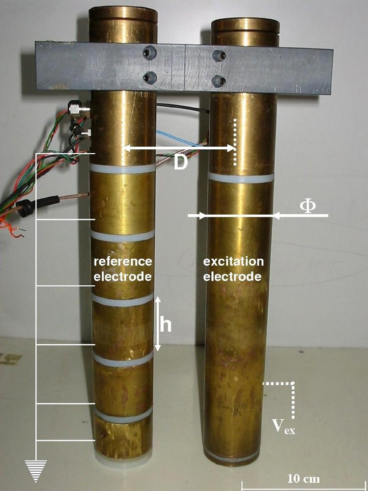
The HYMENET probe (D is the distance between the two electrode axes, Φ the electrode diameter and h the height of one channel of the ground electrode).
La sonde HYMENET (D la distance entre axes des deux électrodes, Φ le diamètre, et h la hauteur d’une voie de mesure sur l’électrode de référence).

The measurement principle of the probe is based on the electrokinetic theory where the soil is considered as a capacitance C in parallel with a resistor R. The geometry of the probe allows accurate measurements of the impedance (and of the apparent soil complex permittivity) in a well-defined significant volume that distinguishes this measurement technique from others [12]. The design is such that the intrinsic dielectric properties of the medium can be derived easily from R and C. The top and bottom parts of the reference electrode ensure that the electric field around the electrodes is horizontal at the intermediate levels (this has been verified by numerical simulations [9]). In these conditions, the four intermediate levels can be considered vertically infinite and the complex impedance is determined as follows [11]:

\begin{array}{c} C = \frac{h π ε_{0} {ε^{'}}_{e f f}}{\arg c h (D / Φ)} & \frac{1}{R} = \frac{h π σ}{\arg c h (D / Φ)} \end{array}

(8)

where arg ch is the inverse hyperbolic cosine function.

From Eq. (8), we determined for each channel the capacitance and the resistor: $C (pF) = 1.04 \times {ε^{'}}_{eff}$ and R(Ω) = 9.2.σ^-1. Values of ${ε^{'}}_{eff}$ ranging from 3 to 50 [4], lead to capacitance values from 3 to 50 pF. For soil bulk conductivity ranging from 0 up to 0.5 S.m^- ¹, the associated resistor value varies from infinity down to 20 Ω.

3.2 Measurement principle

The HYMENET probe is not yet a compact system for field studies. For laboratory work, different devices are used to power the apparatus (DC power supply HP E3631A), send the exciting voltage (Agilent generator up to 80 MHz HP 33250A), digitise and record the different signals (Tektronix numerical scope TDS 3012B with analogue filter at 100 MHz, sampling frequency up to 1 G samples.s^-1, 8 bit nominal resolution and sensitivity down to 10 mV in full scale). The scope works with a numerical filter at 20 MHz and performs an average over 512 scope recordings to reduce the noise to signal ratio. Data are stored in a computer for further estimation of the complex impedances and the dielectric properties of the medium.

A system of remotely operated relays and switches are used to measure successively the voltage and the current (via a trans-impedance) for each channel. Relays are controlled by a shift register driven by a computer with TTL signals. The technical details of the measurement chains are described in the patent [12].

The upper working frequency of the probe is limited to around 20 MHz, as higher frequencies would induce major electronic drawbacks like parasitic self-inductances of conductors. These disturbances grow roughly linearly with the size of the sensor. Consequently, capacitors and self-inductors form resonators amplifying high frequency noises that induce voltage drops, which modify the signal. A careful circuit design permitted control of the main instabilities of the probe by avoiding ground loops and adding low-band filters.

The calibration tests consist in connecting a standard impedance between the electrodes to determine the systematic probe errors. The remaining systematic errors are due to self-inductance of conductors (leads are necessary to connect the standard impedances), parasitic capacitance between close conductors, probe radiation losses and wire skin effect and interferences between channels. Such errors increase with both frequency and impedance discrepancy between channels.

Corrections associated with the determination of impedances from voltage measurements have to be made: parasitic effects induced in the electronic components from a few MHz have to be considered. These parasitic effects are represented by a physical model (equivalent electric circuit) including self-inductances and capacitances. The parameter values of this model are determined through standard electronic components (capacitances composed of ceramic multilayer by American Technical Ceramics, accuracy ± 1%; resistors are 1206 thick film components manufactured by Vishay, accuracy 0.1 %). The parameters involved in this model are highly independent of the studied medium.

3.3 Experimental results

Several experiments were set up to validate the instrument. Before measuring the complex impedance of a soil, we measured certified electronic components (resistors and capacitances) with the HYMENET probe; they were connected to both electrodes using resistance values ranging from 25 to 5000 Ω, and capacitance values from 5 to 70 pF. Different configurations were tested: components alone, combinations of elements in parallel and series (complex impedances), and cross-talk test (influence of impedance measurements on a single channel when other impedances are connected). Fig. 2 presents a comparison between HYMENET measurements and certified component values at frequencies 10 and 20 MHz. The comparison results highlight that measurements of complex impedances with the HYMENET probe agree very satisfactorily with the known impedance values. The maximum measurement error is around 1% in the 1–20 MHz domain, and reaches 5% in the extreme case of high impedance difference between two neighbouring channels (corresponding to one channel in air whereas the other is in a wet medium).

Fig. 2
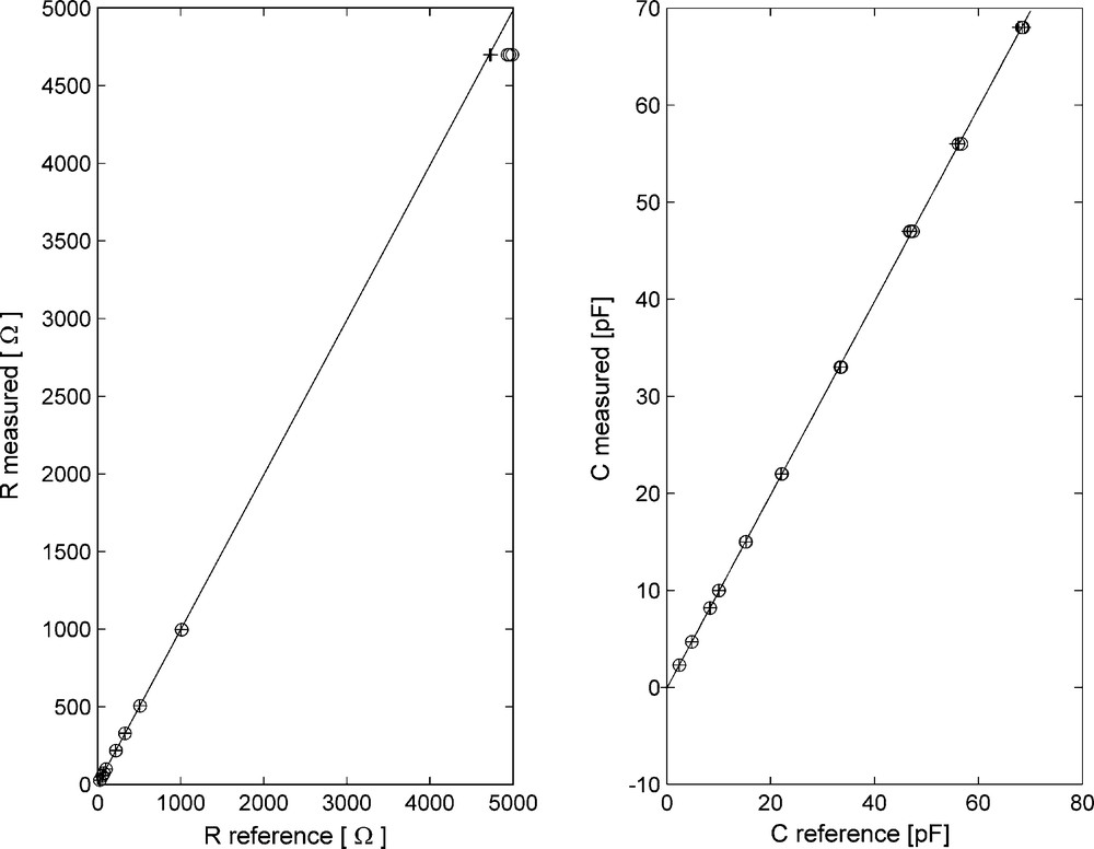
Measurements of complex impedances from certified electronic components (resistances on the left, capacitances on the right) for 10 MHz (+) and 20 MHz (o) using the HYMENET probe.
Mesures d’impédances complexes avec la sonde HYMENET (à gauche, mesures de la résistance, et à droite mesures de la capacité) à 10 MHz (+) et 20 MHz (o), à partir de composants électroniques certifiés.

Afterwards, a laboratory experiment consisted in comparing the real permittivity ${ε^{'}}_{eff}$ issued from HYMENET measurements by using Eq. (8) with another device (such as TDR, Enviroscan (Sentek, Australia), or HMS9000 (SDEC, Reignac-sur-Indre, France [5]) probes). The container in which the measurements were made is a rectangular PVC (length 56 cm, width 36 cm, height 7 cm) filled with Fontainebleau sand (SiO₂ > 99.8%, grain-size distribution between 150 and 250 μm) previously dried in an oven heated to 107 °C for 24 hours. The HMS9000 probe offers the advantages of having a compact design adapted to the container, and of working at a fixed frequency of 39 MHz. Two holes were drilled in the container to insert the HYMENET probe. Distilled water was added gradually to obtain a volumetric water content θ up to 0.45 cm³.cm^-3 (the electric conductivity ranges from 0.5 × 10^-4 to 5 × 10^-4 S.m ^-1). To obtain an average value of the apparent real permittivity, 10 measurements per water content were recorded with the HMS9000 probe at different positions in the container. Fig. 3 shows the results obtained with the HYMENET probe for both frequencies 10 and 20 MHz. A very good correlation between ${ε^{'}}_{eff}$ values issued from both instruments was observed. Concerning the measurements at 10 MHz, the coefficients of the straight-line fit lead to a slope value of 0.833 ± 0.051 and an intercept value of –0.174 ± 0.580 with the square of the correlation coefficient R² = 0.991. For those obtained at 20 MHz, the slope is equal to 0.871 ± 0.052, and the interception point is 0.413 ± 0.586 with R² = 0.991. The existence of a bias between HYMENET and HMS9000 measurements is not really understood, as we cannot tell which instrument is responsible for measurement uncertainties at this stage. The HMS9000 measurements may be disturbed by the proximity of the electric field created by the HYMENET probe, and by the salinity effect on permittivity measurements above 0.5 S.m^-1. Similarly, the HYMENET probe may be disturbed by the current injection of the HMS9000 probe. Additional experiments have shown that real permittivity measurements issued from the HYMENET probe do not seem to be influenced by the conductivity of the medium (this instrument is an impedance meter first and foremost). This bias could be minimized as moisture estimations require a calibration relation when permittivity is measured in situ. To test the accuracy of the probe, standard liquids (such as acetic acid CH₃COOH ${ε^{'}}_{eff} = 6.18$ at 24 °C, ethanol C₂H₅OH ${ε^{'}}_{eff} = 24.3$ at 25 °C and methanol CH₃OH ${ε^{'}}_{eff} = 32.63$ at 25 °C…) and their mixtures can be used [16,17].

Fig. 3
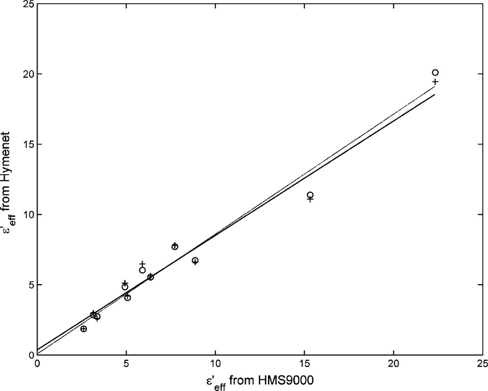
Comparison between the real permittivity measured and associated with a pure sand (Fontainebleau, France) with an increasing moisture content between two probes, the HMS9000 probe (abscissa) at 39 MHz and the HYMENET probe (ordinates) at 10 MHz (+) and 20 MHz (o); the straight lines are plotted for both frequencies (solid line for 10 MHz, and dotted line for 20 MHz).
Comparaison des mesures de permittivité réelle d’un sable pur (Fontainebleau, France), de teneur en eau croissante, issues des sondes HMS9000 (abscisses) à 39 MHz et HYMENET (ordonnées) à différentes fréquences (+ : 10 MHz ; o : 20 MHz) ; les droites de régression linéaire sont tracées pour les deux fréquences (ligne continue pour 10 MHz et ligne discontinue pour 20 MHz).

At this point, the ability of the HYMENET probe to measure moisture in a soil was studied. The experiments made for this purpose have been widely used by other authors [2,5,14,15,21,29], and, as a first step, the relation between the volumetric moisture content and the real permittivity has been studied for the Fontainebleau sand. The experimental protocol is identical to that used to compare the HMS9000 and HYMENET probes. The Fontainebleau sand previously dried in an oven was wetted successively with a defined volume of distilled water and then homogenized. Adding NaCl, the volumetric water content θ was varied up to 0.45 cm³.cm^-3 and the electric conductivity σ ranged from 0.5 × 10^-4 to 5 × 10^-4 S.m^-1. Fig. 4 reveals that HYMENET measurements follow the trend of the Topp's modelling (Eq. (5)), but the curves do not appear superimposed. The differences found between the Topp calibration curve and the HYMENET data is due to the fact that Topp's relation is valid for a certain class of soils only – therefore not valid for pure quartz sand such as Fontainebleau sand. Moreover, the presence of air bubbles in the porous medium may have altered our measurements. The same behaviour for pure sand (Fig. 9) was observed with the monopole probe described below.

Fig. 4
Real permittivity of pure sand (Fontainebleau, France), measured by the HYMENET probe at different frequencies (+: 10 MHz; o: 20 MHz) as a function of the volumetric water content; Topp's relation is plotted in a solid line.
Permittivité réelle d’un sable pur (Fontainebleau, France) mesurée par la sonde HYMENET (+ : 10 MHz ; o : 20 MHz), en fonction de la teneur en eau volumique ; la relation de Topp est tracée en ligne continue.

Fig. 9
Comparison of the estimations of the real permittivity using the resonant frequency algorithm and the Prony approach for a pure sand and a clay sand (o: Prony estimations, *: estimations from resonant frequency algorithm, [light grey line: third-degree polynomial fit, dark grey line: CRIM fit]).
Comparaison des estimations de permittivités réelles obtenues à partir de l’algorithme des fréquences de résonance et de l’algorithme de Prony, dans le cas d’un sable pur et d’un sable argileux (o : estimations par Prony, * : estimations par l’algorithme des fréquences de résonance [tracé gris clair : lissage par polynôme d’ordre 3 ; tracé gris foncé : lissage par CRIM]).

4 The monopole probe

4.1 Probe geometry

The monopole probe, as visualized in Fig. 5a and b, is composed of a radiating thin-wire element of length h = 6 cm with radius a = 0.5 mm that is positioned on a circular disk with a radius of d = 15 cm. Both components are supposed to be infinitely conductive. The antenna is fed back by a coaxial transmission line with impedance Z₀. The choice of both parameters h and d appears as a trade-off: the monopole has to show a minimum of three resonant frequencies in a given soil, and the disk that serves as a ground plane has to be sufficiently large to be assumed infinite. In our approach, the determination of the real permittivity is based on the positions of these first three resonant frequencies. This requires EM modelling that leads to the development of an inversion algorithm.

Fig. 5
Antenna geometry (a) Front view, and (b) cut view.
Géométrie de l’antenne (a) vue de dessus, et (b) vue en coupe.

4.2 Antenna modelling

Two types of electromagnetic modelling were adapted to describe the behaviour of the monopole probe: an analytical one based on Wu's relations [24,38], and a numerical one based on the FDTD approach.

The fundamental models associated with a monopole probe positioned on a conductive ground plane have been collected by Weiner [37]: Richmond's (1984) Method of Moments (MoM) (radius d not too large compared to the wavelength λ in the given medium), the Adwadalla-Maclean's (1979) Method of Moments combined with the Geometrical Theory of Diffraction (GTD) (d ≥ λ), Storer's (1951) variational method (d ≫ λ), and the method of images ( $d \to \infty$ ). In general, the results show that, to be assumed infinite, the diameter d of the disk should at least be equal to 4 λ which usually represents a large dimension as compared to the dimension of the resonant wire element at a given resonant frequency $(2 n + 1) λ / 4$ (n is a positive integer). If the disk radius can be assumed infinite, the method of images is valid, thus leading to simplified models whose validity depends on the ratio h/λ (λ is the wavelength in the given medium) of the monopole length relative to the real wave number β [37]: the short monopole model [32], Wu's long antenna model [24,37] ( $β h \geq 1$ ), and the induced EMF method [25] ( $l / λ \leq 1 / 4$ or $l / λ \leq 1$ ).

Wu's modelling, which considers the radiation of a long thin-wire dipole antenna (a/λ ≪ 1, a/h ≪ 1 and h > λ) immersed in a dielectric and dispersive medium, appears to be well suited to our problem. In our case, assuming an infinite ground plane in the presence of a monopole antenna, the theory of images can be applied and Wu's theory can be used. In the present case, the complex input impedance $\tilde{Z} 11 (ω)$ of the antenna developed analytically by Wu has to be divided by 2. The expression is the following:

\tilde{Z} 11 (ω) = \frac{ω μ_{0}}{j 4 k (S + C U)} [Ω]

(9)

The parameters involved in the definition of C, U and S are defined in [24]; they depend on the product of the wavelength in the medium surrounding the antenna by its length h. The complex wave number in the medium is written:

k = β + j α = ω \sqrt{μ_{0} ε_{0}} {({ε^{'}}_{eff} + j \frac{σ}{ω ε_{0}})}^{1 / 2}

(10)

Since the input impedance $\tilde{Z} 11$ cannot be measured directly by a VNA, it is measured in terms of the reflection coefficient $\tilde{S} 11$ at the antenna feed point according to Eq. (3).

Afterwards, numerical simulations based on the FDTD approach have been developed with the commercial software EMPIRE (IMST, Kamp-Lintfort, Germany). The modelled structure can be visualized in Fig. 5a: the wire element is immersed in an upper semi-infinite dielectric layer (z ≥ 0) representing the soil; its complex permittivity can be described with any usual frequency variation law (Debye, Cole-Cole…). A semi-infinite layer of air is positioned in the lower horizontal part ( $z \leq 0$ ). At all boundaries of the structure, Perfect Matched Layered (PML) conditions have been defined. The source, assumed to be punctual and directed along axis 0z, has been positioned between the bottom end of the wire element and the circular ground plane (thickness e = 0.01 mm).

To further understand the physical phenomena involved when the antenna is immersed in a dissipative medium, we studied the influence of several parameters such as the disk radius, the antenna length, and the real and imaginary parts of the complex permittivity. As an illustration (Fig. 6), comparisons of the results from the analytical and the numerical (FDTD) models for real permittivity values ranging from 1 to 9 ( ${ε^{″}}_{eff} = 0$ ) show that the positions of the first resonant peaks calculated by both models appear very close. We observed a frequency shift (not really explained) for the other resonant peaks between the numerical modelling and the analytical one towards the lower frequencies for ${ε^{'}}_{eff} < 5$ , and towards the higher frequencies for ${ε^{'}}_{eff} \geq 5$ . Moreover, we remark that the analytical modelling does not reproduce an amplitude decrease of $S 11 (d B)$ associated with the multiple reflections observed along the considered frequency band. Then, studying the influence of the imaginary permittivity by means of the conductivity σ ( ${ε^{'}}_{eff} = 5$ ), we remark from Fig. 7 that a frequency shift of the resonant peaks, as compared to the case where σ = 0, is observed when the conductivity reaches a value higher than $0.05 S. m^{- 1}$ . In general, we observed that the presence of a given conductivity in the medium causes an attenuation of the amplitude $S 11 (d B)$ versus frequency without modifying its shape when σ is not too high (< 0.1 S.m⁻¹).

Fig. 6
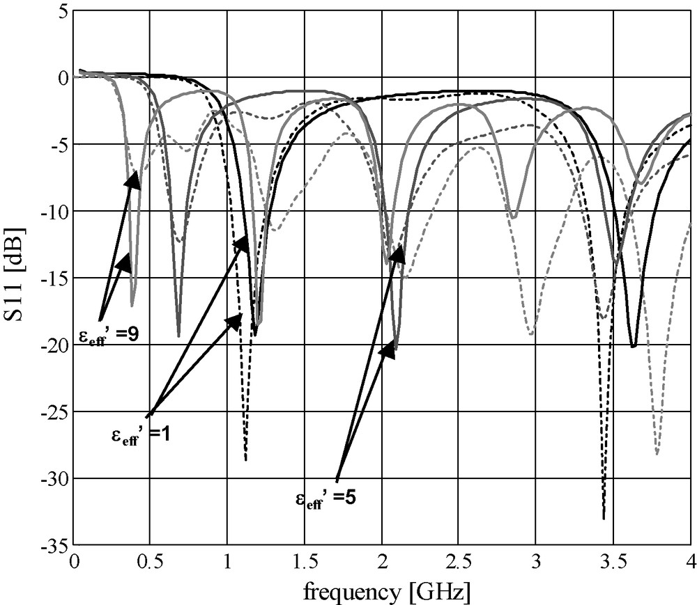
Theoretical reflection coefficients S11(dB) of the monopole probe (h = 6 cm) versus frequency for real permittivity values ${ε^{'}}_{eff} = 1, 5, 9$ ( ${ε^{‴}}_{eff} = 0$ ) (continuous line: analytical modelling, dash-dot line: FDTD modelling).
Coefficients de réflexion théoriques S11(dB) de la sonde monopôle (h = 6 cm), en fonction de la fréquence pour des valeurs de permittivités réelles ${ε^{'}}_{eff} = 1, 5, 9$ ( ${ε^{‴}}_{eff} = 0$ ) (ligne continue : modèle analytique ; ligne en traits-points : modèle FDTD).

Fig. 7
Theoretical reflection coefficients S11(dB) of the monopole probe (h = 6 cm) versus frequency for conductivity values $σ = 0, 0.05, 0.5$ ( ${ε^{'}}_{eff} = 5$ ) (continuous line: analytical modelling, dash-dot line: FDTD modelling).
Coefficients de réflexion théoriques S11(dB) de la sonde monopole (h = 6 cm), en fonction de la fréquence pour des valeurs de conductivités $σ = 0; 0,5; 0,5$ ( ${ε^{'}}_{eff} = 5$ ) (ligne continue : modèle analytique ; ligne en traits-points : modèle FDTD).

4.3 Inversion algorithms

To estimate the average complex permittivity of a given soil in a wide frequency band, we developed two different algorithms: one based on the resonant frequencies, and the other on the high resolution Prony model [28,30]. The approach based on the resonant frequencies considers only the positions of the discontinuities in the variation of the reflection coefficient versus frequency, whereas the Prony approach aims at fitting the reflection coefficient variations to its discontinuities using a multipath propagation model.

4.3.1 The resonant frequency algorithm

This algorithm consists of several steps:

• Detection and selection of local minima (resonant frequencies) of the experimental curve $|S 11 (f)|$ under study and associated with an unknown value of the real permittivity value ${ε^{‴}}_{eff} = 0$ (low-pass interpolation of the 17 nearest frequency samples around each minimum);
• Plotting the variation of the first three resonant frequencies (index i) as a function of the real permittivity for both modelling – analytical and numerical – and determination of the parameters (a_i, b_i) of the curve $f_{i} ({ε^{'}}_{eff})$ fitting the variation of each resonant frequency versus the real permittivity such as:
$f_{i} ({ε^{'}}_{eff}) = a_{i} + \frac{b_{i}}{\sqrt{{ε^{'}}_{eff}}} i = 1,2,3$ (11)
• Determination of the average variation of each resonant frequency versus the real permittivity according to both fitting curves associated with both models;
• Estimation of the real permittivity from the three first resonant frequencies issued from the experimental data of $|S 11 (f)|$ and compared to the average of the three theoretical curves, using the least square criterion.

4.3.2 The Prony-based algorithm

We propose an original application of the Prony-based algorithm that aims to identify the individual paths issued from successive reflections occurring inside the monopole antenna [28,30].

Using the Prony approach, the reflection time response of the probe surrounded by a dielectric medium is modelled as the sum of M individual paths which represent multiple copies of the incident signal, the k-th path being characterized by a complex delay τ_k and a complex attenuation a_k. Considering M paths, the transfer function can be written as follows:

\tilde{H} (ω_{n}) = \sum_{k = 1}^{M} a_{k} e^{- j τ_{k} ω_{n}} ω_{\min} \leq ω_{n} \leq ω_{\max}

(12)

where $ω_{n} = 2 π f_{n}$ .

In the present modelling, the delay τ_k is a complex number defined as follows:

τ_{k} = T_{k} - j α_{k}

(13)

where T_k represents the travel time of path k through the medium, and α_k is the slope of the frequency attenuation. Such a complex delay allows us to take into account the frequency dispersion involved in wideband studies.

The data processing consists in fitting the frequency data (at present, the reflection coefficient S11) to the model (expressed by Eq. (12)) to estimate the complex amplitudes a_k and exponential arguments τ_k of the individual delayed paths k (Fig. 8 in the case of measured data in a pure sand). Two main steps are necessary: first, the exponential argument of each ray is calculated using a Singular Value Decomposition (SVD) of a specific data matrix, followed by the determination of a matrix pencil whose eigenvalues are the M poles ${\tilde{Z}}_{k}$ . Then, the amplitudes b_k are determined using a least-square fitting of the N frequency data.

Fig. 8
Experimental reflection coefficients S11(dB) of the monopole probe (h = 6 cm) measured in the band [0.1 – 3.5] GHz in the presence of a pure sand with several moisture contents by weight w = 0%, 2.7%, 5.3%, 7.4% and fitted by the Prony algorithm (continuous line: experimental data, dash-dot line: Prony fitting).
Coefficients de réflexion expérimentaux S11(dB) de la sonde monopôle (h = 6 cm), mesurés dans la bande [0,1 – 3,5] GHz en présence d’un sable pur comprenant différentes teneurs en eau massiques w = 0 %, 2,7 %, 5,3 %, 7,4 % et lissés par l’algorithme de Prony (ligne continue : données expérimentales ; ligne en traits-points : lissage par Prony).

The average dielectric properties of the surrounding medium can be estimated from the complex propagation times τ_k as follows:

\{\begin{array}{l} {ε^{'}}_{eff} = {(\frac{c}{2 (k - 1) h})}^{2} ({(T_{k} - T_{1})}^{2} - α_{k}^{2}) \\ {ε^{‴}}_{eff} = {(\frac{c}{2 (k - 1) h})}^{2} (2 (T_{k} - T_{1}) α_{k}) \end{array} k = 2, \dots, M

(14)

4.4 Experimental results

The validation of the experimental tool with its inversion algorithms was performed in our laboratory on pure sand (class D1, AFNOR NF P 11-300) and weak clay sand (class B2) from the Stref sandpit (Jumièges, France). Their dielectric properties were studied as functions of the moisture content. By sampling and drying (gamma probe and gravimetric measurements), the gravimetric moisture contents w ranging from 0 to 12.25% were previously estimated. The container in which laboratory measurements were made is a rectangular PVC box (length 56.8 cm, width 36.4 cm, height 40.8 cm) filled with 20 cm of soil. Each type of sand had been previously dried in an oven heated to 107 °C for 24 hours. Then, water was added gradually to reach the different moisture contents. Compaction at a particular moisture content was made, thus leading to densities ρ_h as collected in Tables 1 and 2. For each moisture content, four measurements were made with the monopole antenna at different locations. At the same time, measurements were made of sand samples inside a cylindrical cavity were [20].

Moisture by weight (w)	Resonant frequencies ( ${ε^{'}}_{eff}$ )	Resonant frequencies (Δ ${ε^{'}}_{eff}$ )	Prony algorithm ( ${ε^{'}}_{eff}$ )	Prony algorithm (Δ ${ε^{'}}_{eff}$ )	Prony algorithm (σ [S/m])	Cavity measurement at f₀ = 1.3 GHz ( ${ε^{'}}_{eff}$ [± 5%])	Density by weight ρ_h (kg.dm^-3)
Dry sand	2.56	± 0.144	2.55	± 0.10	2.09 10^-3	2.80	1.7
Moisture 2.65%	2.84	± 0.10	3.12	± 0.10	4.17 10^-3	3.31	1.45
Moisture 5.3%	4.11	± 0.144	4.25	± 0.08	5.38 10^-3	4.31	1.65
Moisture 7.4%	4.82	± 0.14	5.41	± 0.14	7.94 10^-3	5.31	1.58
Moisture 10%	6.09	± 0.14	6.08	± 0.1	1.25 10^-2	6.39	1.62
Moisture 12.25%	7.65	± 0.14	7.35	± 0.1	1.4 10^-2	8.33	1.7

Moisture by weight (w)	Resonant frequencies ( ${ε^{'}}_{eff}$ )	Resonant frequencies (Δ ${ε^{'}}_{eff}$ )	Prony algorithm ( ${ε^{'}}_{eff}$ )	Prony algorithm (Δ ${ε^{'}}_{eff}$ )	Prony algorithm (σ [S/m])	Cavity measurement at f₀ = 1.3 GHz ${ε^{'}}_{eff}$ (± 5%)	Density by weight $ρ_{h}$ [kg.dm^-3]
Dry sand	2.13	± 0.14	2.32	± 0.10	1.89 10^-3	2.88	1.34
Moisture 2.59%	3.40	± 0.14	3.49	± 0.10	3.8 10^-3	3.89	1.54
Moisture 5.07%	4.25	± 0.14	4.40	± 0.10	6.24 10^-3	4.04	1.56
Moisture 7.48 %	6.37	± 0.28	6.47	± 0.20	9.28 10^-3	6.39	1.69
Moisture 9.26%	7.22	± 0.56	7.01	± 0.20	1.36 10^-2	7.87	1.79
Moisture 11.20%	9.48	± 0.35	9.43	± 0.20	1.86 10^-2	9.84	1.81

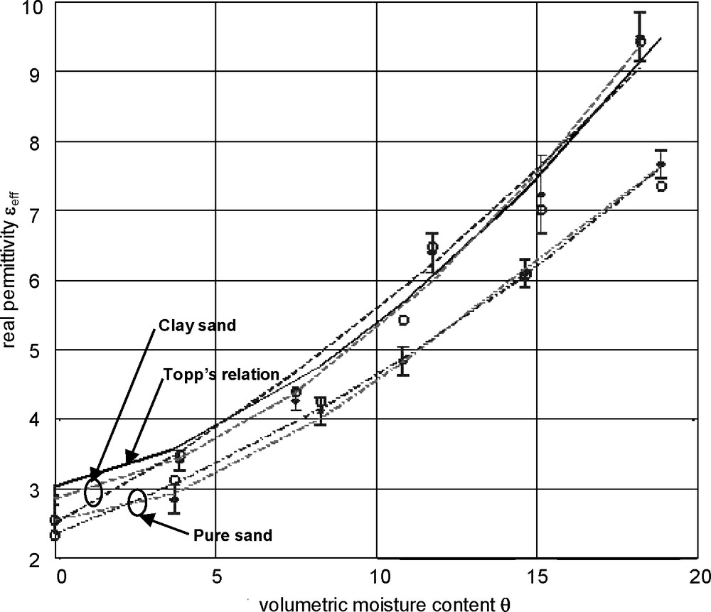
For both sands, the relation between the real permittivity and the volumetric moisture content was expressed using Topp's polynomial and the CRIM relation. As compared to pure sand, Fig. 9 demonstrates that the clay sand shows a greater sensibility to the presence of water, particularly at low volumetric moisture contents (less than 5%); this observation is consistent with its belonging to class B2. As shown in Fig. 9, the variation of the real permittivity with volumetric moisture content of the clay sand agrees quite well with Topp's relation. This is not observed in the case of pure sand because Topp's relation is not well adapted to pure sand as previously mentioned about the corresponding HYMENET measurements in section 3.3. Thus, comparing HYMENET and monopole data for volumetric water contents up to 20 cm³.cm^-3 by using interpolations, we obtain the following linear regression coefficients: a slope value of 0.99, an intercept value of –0.27, and the square of the correlation coefficient R² = 0.99.

The coefficients associated with the third-degree polynomial fitting of the real permittivity estimates by the monopole antenna are A = 2.53, B = 3.02, C = 218.95 and D = −487 for pure sand, and A = 2.85, B = 9.26, C = 149.08 and D = −22.91 for clay sand. In the case of the CRIM fit, assuming K = 1 ( $ρ_{s} = 2.66 g . c m^{- 3}$ and ${ε^{'}}_{s} = 2.56$ ), the coefficient values are α = 1.36, and $C = 1.6 10^{- 3}$ for pure sand, and α = 1.90, and $C = 5.3 10^{- 1}$ for the clay sand. We remark from Table 2 that the clay sand has a conductivity that increases gradually with moisture content.

Moreover, the first measurements presented in Fig. 10 were made with the 6 cm long monopole on a test site at LRPC Rouen. A silt of class A1 was deposited in a 45 m long and 1 m high chamber with three moisture contents (weak, medium, and high corresponding to parts A, C and B respectively) along the chamber length; the average densities of the wet soil measured by a gamma probe in each of the three parts along line H (H8…H12; H23…H27; H38…H42) are 1.88, 1.98, and 1.82 g.cm^-3 respectively. After sampling and heating, the average dry density was measured: ρ_d = 1.73, 1.81, and 1.7 g.cm^-3, respectively. As shown in Fig. 11, the real permittivity values issued from monopole measurements and the developed data processing were compared to the measurements obtained by a commercial TDR probe (TRASE system, Moisture Equipment Corporation, Santa Barbara, CA, USA) with two rods; the average value of the real permittivity for points H9 to H12 was evaluated to 7.6 (medium moisture content w), for points H23 to H27 to 8.7 (high w), and for points H38 to H42 to 6.8 (weak w). In general, the relative dispersion in the estimations observed from Fig. 11 is less than 11%. When estimating the real permittivity with the monopole probe and the two types of inversion algorithms, we observed a relative error of less than 15%. As the wet densities of the three parts A, B and C are not identical, we first used a mean value for ρ_d (1.75 g.cm^-3) in the CRIM relation (7) to fit the data in a narrow range of moisture content θ such as:

{ε^{'}}_{eff} = K {(\frac{ρ_{d}}{ρ_{s}} [{({ε^{'}}_{s})}^{1 / α} - 1] + θ [{({ε^{'}}_{w})}^{1 / α} - 1] + 1)}^{α} + C

(15)

Fig. 10
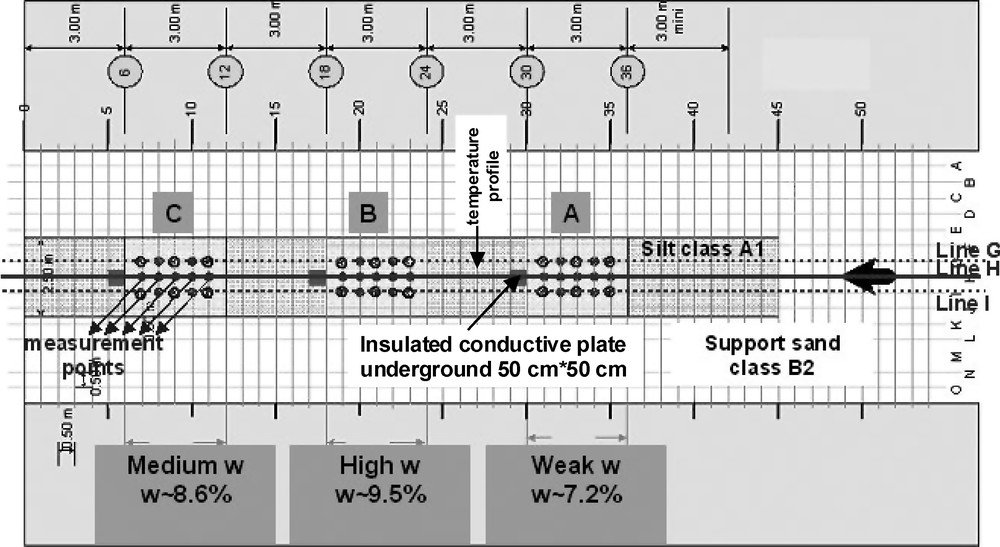
Scheme of the soilboard made of silt (class A1) including 3 parts A, B, and C with different moisture contents w by weight.
Schéma de la planche de sol limoneux (classe A1) comprenant 3 parties A, B, et C se distinguant par leurs teneurs en eau massiques w.

Fig. 11
Estimates of the real permittivity issued from monopole (h = 6 cm) and TDR measurements (+: TDR results; *: resonant frequency algorithm using the monopole; o: Prony algorithm using the monopole).
Estimés de permittivités réelles issues de mesures utilisant la sonde monopôle (h = 6 cm) et la TDR (+ : résultats TDR ; * : algorithme des fréquences de resonance, appliqué au monopôle ; o : algorithme de Prony appliqué au monopôle).

Fig. 12 presents the fits using the CRIM relation for TDR and monopole data (issued from the resonant frequency algorithm). Both fits are based on only three moisture contents, and their comparison shows a weaker slope in the variation of ${ε^{'}}_{eff}$ with θ in the case of TDR data as compared to monopole measurements. Future measurement campaigns will study the influence of the compaction level, and therefore the dry density of the soil for these three soilboard parts.

Fig. 12
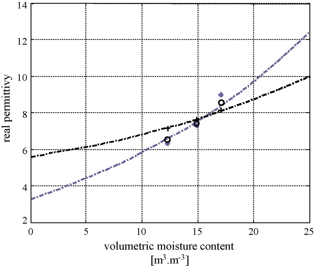
Fitting of the real permittivity estimates (issued from TDR (in black), and the monopole with the resonant frequency algorithm (in grey)) using the extended CRIM relation.
Lissage des estimations de permittivités réelles issues de la sonde TDR (en noir), et de la sonde monopôle (en associant l’algorithme des fréquences de résonance [en gris]) à partir de la relation de CRIM étendue.

5 Conclusion

This paper presents novel instruments dedicated to the characterization of the volumetric moisture content of soils in a large frequency range 1–20 MHz and 0.1–4 GHz respectively. While the HYMENET probe is based on the capacitive effect, the monopole probe is based on the propagation of electromagnetic waves at high frequencies. When inserted into a soil, the input complex impedance of each probe is measured as a function of the frequency. Based on the complex impedance, we used specific algorithms in order to determine the apparent complex permittivity of the soil. Whereas the HYMENET probe is able to measure a real permittivity ${ε^{'}}_{a}$ and a static conductivity σ, the monopole probe can measure the real and the imaginary parts of the permittivities ${ε^{'}}_{eff}$ and ${ε^{‴}}_{eff}$ respectively. From the real permittivity and a calibration step, we can estimate the volumetric moisture content for each type of soil using empirical or semi-empirical relations. First, we presented results concerning the validation of both probes in the presence of known surrounding media, or media that have been measured in parallel by means of other types of instruments. Then, we studied in the laboratory the influence of moisture content in sandy soils on the value of the apparent real permittivity of the soil. In general, with the HYMENET probe the error is less than 5%, and the monopole probe leads to an error below 15% (including pure sand and silty-soil measurements). This difference can be explained by the fact that the monopole probe works at higher frequencies, and that its accuracy includes the results issued from a highly heterogeneous silty soil of class A1. We wish to underline that, at present, the two instruments have been developed and validated separately in the laboratory with two types of pure sand. However, both instruments give very close real permittivity values in the available range [0–10] on pure sand as a function of the volumetric moisture content with a good linear relationship (slope value equal to 0.99, and the square of the correlation coefficient R² = 0.99).

The aim of future work is to measure various soils with the HYMENET and the monopole probes in order to compare their performances at one test site at least. We are particularly interested in compiling a database of soils encountered in civil engineering and geophysical applications.

Acknowledgements

This work was partially supported by INSU/CNRS framework ECCO WATERSCAN and by LCPC programs. The authors would like to thank J.-P. Laurent (LTHE, Grenoble, France) for his relevant remarks, which have helped to greatly improve the manuscript.

Bibliographie

[1] J. Behari, Microwave dielectric behavior of wet soils, Springer (Ed.), 2005, 200 p.

[2] J.P. Bell; T.J. Dean; M.G. Hodnett Soil moisture measurement by an improved capacitance technique, Part II: Field techniques, evaluation and calibration, J. Hydrol., Volume 93 (1987), pp. 79-90

[3] J.R. Birchak; C.G. Gardner; J.E. Hipp; J.M. Victor High dielectric-constant microwave probes for sensing soil-moisture, Proceedings of the IEEE, Volume 62 (1974) no. 1, pp. 93-98

[4] J.E. Campbell Dielectrics properties and influence of conductivity in soils at one to 50 MHz, Soil Sci. Soc. Am. J., Volume 54 (1990), pp. 332-341

[5] A. Chanzy; J. Chadoeuf; J.C. Gaudu; D. Mohrath; G. Richard; L. Bruckler Soil moisture monitoring at the field scale using automatic capacitance probes, Eur. J. Soil Sci., Volume 49 (1998), pp. 637-648

[6] D.J. Daniels Ground penetrating radar, The Institution of Electrical Engineers, London, UK, 2004 (719 p)

[7] J.L. Davis; W.J. Chudobiak In situ meter for measuring relative permittivity of soils; Report of activities, April to October 1974, Geophysics Pap. Geological Survey Can., Volume 75–1 (1975), pp. 75-80

[8] G.P. de Loor The dielectric properties of wet soils, IEEE Trans. Geosc. Remote Sensing GE-21 (3) (1983), pp. 364-369

[9] G. de Rosny; A. Chanzy; M. Pardé; J.C. Gaudu; J.P. Frangi; J.P. Laurent Numerical modeling of a capacitance probe response, Soil Sci. Soc. Am. J., Volume 65 (2001), pp. 13-18

[10] M.C. Dobson; F. Kouyate; F.T. Ulaby; M.T. Hallikainen; M.A. El Rayes Microwave dielectric behaviour of wet soil - Part II: Dielectric mixing models, IEEE Trans. Geosc. Remote Sens., Volume 23 (1985) no. 1, pp. 51-61

[11] E. Durand Électrostatique, Masson (Ed.), Paris, France, 1966 (389 p)

[12] J.P. Frangi, G. de Rosny, X. Chavanne, D. Richard, A. Bruère, Device for measuring electrical properties of a water-containing medium. World Intellectual Property Org. WO/2008/006973, Patent PCT/FR2007/01180, 17 January 2008.

[13] E. Fratticcioli, M. Dionigi, R. Sorrentino, A new permittivity model for the microwave moisture measurement of wet sand, 33^rd European Microwave Conference, Munich, Germany, (2003) 539–542.

[14] C.M.K. Gardner; T.J. Dean; J.D. Cooper Soil water content measurement with a high-frequency capacitance sensor, J. Agric. Eng. Res., Volume 71 (1998), pp. 395-403

[15] G.J. Gaskin; J.D. Miller Measurement of soil water content using a simplified impedance measuring technique, J. Agric. Eng. Res., Volume 63 (1996), pp. 153-160

[16] Handbook of chemistry and physics, 67th ed., CRC (Ed.), 1986–1987.

[17] J.B. Hasted Aqueous dielectrics, Chapman and Hall (Ed.), 1973 (302 p)

[18] C. Hignett, S.R. Evett, Neutron Thermalization, Section 3.1.3.10, In: Jacob H. Dane and G. Clarke Topp (Eds.), Methods of Soil Analysis, Part 4-Physical Methods (2002) 501–521.

[19] T.J. Jackson; T.J. Schmugge Surface soil moisture measurement with microwave radiometry, Acta Astronaut., Volume 35 (1995), pp. 477-482

[20] S. Li; C. Akyel; R.G. Bosisio Precise calculations and measurements on the complex dielectric constant of lossy materials using TM010 cavity perturbation technique, IEEE Trans. Microwave Theory Techn. MTTT-29(10) (1981), pp. 1041-1047

[21] H. Magán; R. Ordiales; M.A. Domene; S. Vidal Self balance impedance bridge, un método alternativo al TDR para la determinación de la humedad edáfica, Ecosistemas, X (3) (2001), pp. 29-36

[22] C.G. Malmberg; A.A. Maryott Dielectric constant of water from 0 °C to 100 °C, J. Res. Nat. Bur. Stand., Volume 56 (1956), pp. 1-8

[23] V.L. Mironov; M.C. Dobson; V.H. Kaupp; S.A. Komarov; V.N. Kleshchenko Generalized refractive mixing dielectric model for moist soils, IEEE Trans. Geos. Remote Sens., Volume 42 (2004) no. 4, pp. 773-785

[24] S.C. Olson; M.F. Iskander A new in situ procedure for measuring the dielectric properties of low permittivity materials, IEEE Trans. Inst. Meas., IM-35(1) (1986), pp. 2-6

[25] D.V. Otto A note on the induced EMF method for antenna impedance, IEEE Trans. Antennas Propagat. (1969), pp. 101-102

[26] N.R. Peplinski; F.T. Ulaby; M.C. Dobson Dielectric properties of soils in the 0.3–1.3 GHz range, IEEE Trans. Geosc. Remote Sens., Volume 33 (1995) no. 3, pp. 803-807

[27] D. Polder; J.H. van Santen The effective permeability of mixtures of solids, Physica, Volume 12 (1946) no. 5, pp. 257-271

[28] R.C. Qiu; I.T. Lu Multipath resolving with frequency dependence for wide-band wireless channel modelling, IEEE Trans. Veh. Technol., Volume 48 (1999) no. 1, pp. 350-354

[29] W.S. Rial; Y.J. Han Assessing soil water content using complex permittivity, Trans. ASAE, Volume 43 (2000), pp. 1979-1985

[30] T.K. Sarkar; O. Pereira Using the matrix pencil method to estimate the parameters of a sum of complex exponentials, IEEE Antennas Propag. Mag., Volume 37–1 (1995), pp. 48-55

[31] W. Skierucha; R.T. Malicki TDR method for the measurement of water content and salinity of porous media (W. Skierucha; R.T. Walczak, eds.), Institute of Agrophysics PAS, Lublin (Poland), 2004

[32] G.S. Smith; J.D. Nordgard Measurement of the electrical constitutive parameters of materials using antennas, IEEE Trans. Antennas Propagat. AP-33 (1985), pp. 783-792

[33] G.C. Topp; J.L. Davis; A.P. Annan Electromagnetic determination of soil water content: Measurements in coaxial transmission lines, Water Resour. Res., Volume 16 (1980) no. 3, pp. 574-582

[34] R. Valckenborg NMR on technological porous materials, Eindhoven University, 2001 (123 p)

[35] A. Valente; R. Morais; C. Couto; J.H. Campbell Modeling, simulation and testing of a silicon soil moisture sensor based on the dual-probe heat-pulse method, Sensors Actuators A: Physical, Volume 115 (2004), pp. 434-439

[36] J.R. Wang; T.J. Schmugge An empirical model for the complex dielectric permittivity of soils as a function of water content, IEEE Trans. Geosc. Remote Sens., Volume 18 (1980), pp. 574-582

[37] M.M. Weiner Monopole antennas, Marcel Dekker (Ed.), New York, USA, 2007 (768 p)

[38] T.T. Wu Theory of the dipole antenna and the two-wire transmission line, J. Math. Phys., Volume 2 (1961) no. 4, pp. 550-557