

1 Introduction
It is well known that carbon dioxide (CO2) concentration is rising in the atmosphere as a result of anthropogenic activities: Fossil fuel burning, cement production and forest clearing. Recent estimates are emissions of 7.9 GtC/yr due to fossil fuel and cement productions in 2005, while forest clearing leads to a net flux to the atmosphere of 1.5 GtC/yr (Raupach et al., 2007). On the other hand, the atmospheric load of CO2 shows a net increase of 4.2 GtC/yr on average with very large annual fluctuations. There is, therefore, a natural net sink of CO2 into the oceans and the land ecosystems. Best estimates lead to an almost even partition with 2.2 GtC/yr to the oceans and 2.3 GtC/yr to land surfaces, albeit with rather large uncertainties on each of the numbers (while their sum is rather well constrained).
A similar picture exists for methane (CH4). Methane is emitted by human activities in the energy sector (coal and gas extraction), in the agricultural sector (rice paddies, animals) and by natural processes as well (wetlands, wildfires). However, unlike for carbon dioxide, the ocean-atmosphere flux of methane is insignificant. Methane is massively removed from the atmosphere by photochemical processes. After a rapid increase during the 20th century, the atmospheric concentrations of methane have levelled off a decade ago, for reasons that are still to be understood although some hypotheses exist (Bousquet et al., 2006) Large fluctuations in the growth rate of atmospheric methane are also observed from one year to the next, but their causes remain uncertain.
The spatial distribution of the CO2 sinks is a matter of debate. It is not clear whether the largest sink of CO2 is in the tropics, in the mid-latitudes or in boreal and arctic regions. The repartition in longitude among the continents is also a subject of large controversies. The spatial distribution of CO2 emissions and sinks can be seen as a political question when a state claims that its natural sinks are larger than its net anthropogenic flux to the atmosphere. However, the need is mostly a scientific question for a better understanding of the processes that control the carbon flows between the various reservoirs, and their interactions with the climate system. A better knowledge of today's CO2 fluxes at the regional scale would permit discriminating among various ecosystem and ocean models that claim rather different carbon exchanges.
This science question (i.e., the development and validation of accurate carbon cycle models for the natural exchanges between the various reservoirs) has a strong societal impact. Indeed, the current sink limits the growth rate of the greenhouse effect and therefore of climate change. The current sink is observed to decrease sharply during particularly dry years like 1998, 2002, 2003, 2005. There are reasons to fear that this sink could decrease in the future, and even reverse as a result of climate change. This is because vegetation could react negatively to temperature increases or drought in the tropics, and because high-latitude carbon stocks could decompose faster with warmer temperatures. Thus, for a prediction of the rate of climate change during the 21st century, there is a need for better models of the carbon cycle. Clearly, an accurate description of current fluxes and their variability would be a great help for the validation, the development and further improvement of such carbon models.
Beyond the scientific goal of monitoring carbon fluxes, there is also a political need to establish accurate observing systems for quantifying sources and sinks of greenhouse gases on national levels in the context of the Kyoto protocol and its likely successors. The accuracy requirements for this goal are substantially higher than for the scientific objectives mentioned above, because fluxes over relatively small geographical units and long time periods (e.g., 5-year commitment periods) have to be quantified. Furthermore, smaller changes in flux magnitudes have to be detected. Nevertheless, any global monitoring strategy has also to address this political objective.
Carbon dioxide is the main contributor to the radiative forcing of the Earth, which leads to climate change. The following contributors are methane and nitrous oxide (IPCC, 2007). Similarly to CO2, there are large uncertainties on the sources of CH4 and N2O. Therefore, the discussion above also applies to these gases although their impact on climate change is less than that of CO2 partly because of the magnitude of the emissions, and partly because of the shorter life times (in case of CH4). Another significant difference between CH4/N2O and CO2 is the large biogenic sink of CO2 from photosynthesis and ocean uptake. Therefore, uncertainties on CH4 and N2O fluxes are primarily on the sources, and not on the sinks.
2 The need for a monitoring of greenhouse gas concentrations
There are several ways to estimate the fluxes of CO2. One method is to make direct measurements from towers above various ecosystems using eddy covariance methods. There are over 300 such stations in the world, coordinated through the fluxnet project [www.eosdis.ornl.gov/FLUXNET/]. These stations measure fluxes of carbon dioxide, water vapour, and heat between terrestrial ecosystems and atmosphere. Researchers also collect data on site vegetation, soil, hydrologic, and meteorological characteristics at the tower sites. Although very useful to constrain the models over specific, well-documented biomes, the stations provide measurements that are local in nature and not necessarily representative of the local or the global scale.
Another method is to sample carbon stocks at various intervals and deduce the flux from the temporal change in stocks. For instance, it is possible to measure the tree growth over several years. Although such methods are needed to monitor the long-term variations of carbon stock, they are necessarily local and difficult to extrapolate at the regional scale, in particular over heterogeneous areas. Further, soil C stocks are very seldom measured. The large size and large heterogeneity of the soil reservoir imposes very long sampling intervals in order to be able to detect a significant change.
The third method is to use atmospheric CO2 concentration at various stations distributed around the globe. The spatial and temporal gradients of CO2 concentration are directly related to surface fluxes. Thus, through a so-called atmospheric transport inversion model, it is possible to estimate the spatial distributions of the fluxes that are in best agreement with the atmospheric concentrations (Bousquet et al., 2006). Clearly, the spatial resolution that is accessible with inversions directly depends on the density (in space and time) of the data. Besides, the inversion method requires an accurate description of the atmospheric transport, including the vertical mixing. At present, such method has been used to estimate the surface fluxes at continental scales from a network of about 100 stations. As a response to the growing interest in carbon fluxes, the network is expanding rapidly. In addition, the temporal density is increasing from measurements at typically biweekly intervals to continuous sampling. Regions where such a dense network of continuous sampling sites exists are Europe and North America.
Despite the continuous expansion of the in situ monitoring network, it is clear that it will never have the density required for global monitoring of fluxes at a fine scale, say of 100 km. Moreover, the in situ monitoring network will not be expandable with adequate density over the oceans, and over large forest areas difficult to access (Amazon, Africa, Siberia). In this context, the use of spaceborne observations is appealing (Chevallier et al., 2007; Palmer, 2008). Indeed, spaceborne observations complement the in situ network by bringing a high density of measurements over most of the Earth. Besides, spaceborne observations are free from local pressure and can therefore provide a uniform coverage, even over regions difficult to access.
However, a satellite estimate of atmospheric concentrations for monitoring of sources and sinks faces a number of challenges, the primary one being accuracy. Indeed, CO2 and other major greenhouse gases are long-lived. Long-lived means that the time scale of atmospheric mixing is much less than the residence time in the atmosphere. As a consequence, the concentration gradients that are generated by local sources and sinks are small in comparison to the background concentration. A very high relative accuracy is therefore necessary, and such accuracy is difficult to achieve from space.
Ideally, a vertical profile of the greenhouse gases concentration would be desirable. Indeed, a full knowledge of the vertical distribution brings additional information on the source and sinks location. However, none of the currently envisioned remote sensing techniques allows the retrieval of such vertical distribution. Rather, a mean column concentration is retrieved, which is often referred to, in the case of CO2, as XCO2:
| (1) |
| (2) |
Surface fluxes impact primarily the concentration in the lowest atmosphere, i.e., the boundary layer. Convection and atmospheric transport mix the air higher up over a longer period, typically a few days. Although theoretically possible, it is then more difficult and chiefly more uncertain to relate concentration gradients in the upper atmosphere to surface fluxes. Therefore, it is highly desirable that the retrieved XCO2 has a strong sensitivity to the low atmosphere or, in different words, that the weighting function takes values close to or larger than 1 for pressures close to that of the surface.
Fig. 1 shows theoretical weighting function for several instruments that are used or planned for the monitoring of carbon dioxide from space. Instruments that operate in the thermal infrared have a weighting function that peaks much higher than those operating in the solar infrared, as will be discussed below.
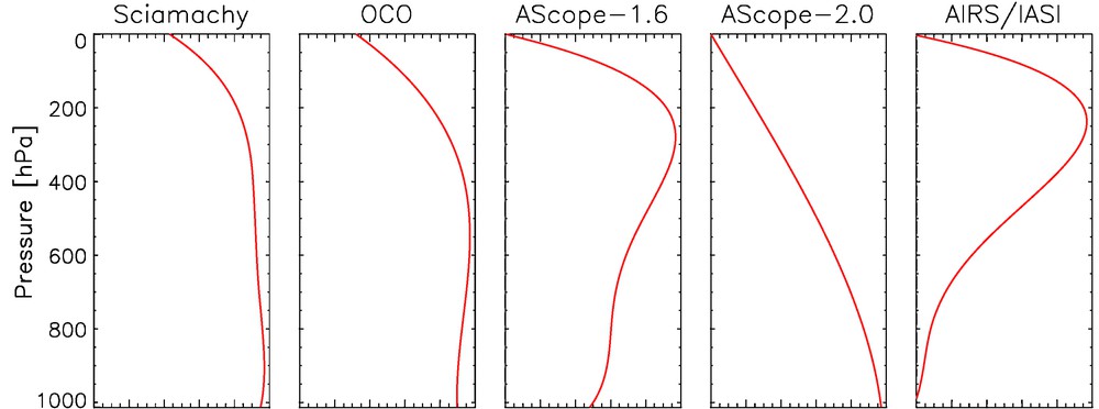
Vertical Weighting Functions w[p] (Eq. (1)) for several instruments that are used or planned for the remote sensing of CO2 from space. Note that the weighting functions slightly depend on the data analysis procedure and the geophysical conditions (temperature profile, atmospheric aerosol, surface albedo…). Typical functions are shown here.
Fonction de pondération verticale w[p] (Éq. (1)) pour plusieurs instruments qui sont utilisés ou envisagés pour la mesure du CO2 depuis l’espace. Les fonctions de pondération dépendent légèrement de la méthode d’analyse des données, ainsi que des conditions géophysiques (profil de température, profil des aérosols, albédo de surface…). Des fonctions typiques sont montrées ici.
3 Three potential technique for the measurement of greenhouse gases concentrations
There are three identified techniques for the estimate of atmospheric concentration of greenhouse gases from space. Two of them are passive while the third one is based on a lidar. In the following, we detail these techniques. Spaceborne missions that use these techniques are described in the next section.
3.1 Thermal infrared sounding
In the thermal infrared (wavelength greater than 4 μm), the radiance emitted by the atmosphere is very much a function of its temperature. On the other hand, it is also function of its composition.
The radiance I(λ) measured at the top of the atmosphere at wavelength λ can be written:
| (3) |
| (4) |
In Eq. (3) the first term is the surface contribution which is proportional to the surface emissivity ɛ(λ). The second term is the atmospheric contribution. It is the integral of the Planck function over the atmospheric column weighted by the derivative of the transmission. By selecting the wavelength, one can choose different levels of absorption, from transparent channels (τ(Psurf) ≈ 1 ) up to highly absorbing channels(τ(Psurf) ≈ 0 ). For absorbing channels, the weighting function in the atmospheric term is close to zero both in the boundary layer and in the highest atmospheric levels. There is a level in the atmosphere where it takes its maximum value. The channel “sees” preferentially this particular level. The weighting function ∂τ/∂p extends over several kilometres around the level where it takes its maximal value. By selecting different channels with different absorbing levels, one can probe different levels in the atmosphere.
For a given wavelength, the absorption KP(λ,T,p) depends on the atmosphere composition (concentration of the absorbing gases), and on temperature and pressure. If the concentration of the absorbing gases is known, the radiance measurements may be used for an estimate of the atmospheric temperature profile. This measurement concept has been used for nearly three decades to retrieve atmospheric temperature profiles from the TOVS instrument package onboard the operational NOAA satellites. It is now used for the same purpose with the instruments IASI and AIRS. Note that some of the temperature profile estimates make use of CO2 absorption bands and the retrieval technique assumes in that case that CO2 concentration is known.
Conversely, if the atmospheric temperature profile is known, one may deduce from the measurements the absorbing gas concentration from the inferred K. Basically, as the gas concentration gets larger, the channel of interest sees higher in the atmosphere and, for a troposphere peaking channel, the measured radiance corresponds to a colder temperature. By adjusting the measured and modelled radiance using the known temperature profile, the absorbing gas concentration can be estimated. The main uncertainty is the knowledge on the temperature profile. Note also that, although some vertical profiling information can be obtained by using different channels, the vertical resolution is not better than a few kilometres. Finally, the technique usually requires channels with a significant absorption so that there is negligible contribution from the surface. As a consequence, the measurement sensitivity to the lower atmospheric layers is comparatively small (Engelen and Stephens, 2004).
3.2 Solar spectroscopy
In the emission spectroscopy technique, the wavelength range is in the thermal infrared. In the thermal infrared, the radiance emitted by the Earth (surface + atmosphere) is significantly larger than that emitted by the sun and reflected by the Earth. At shorter wavelengths (λ < 3 μm), the opposite is true. In this spectral range, there is no significant emission, neither by the surface nor by the atmosphere (we exclude here marginal cases of city light and fires). Earth observing satellite instruments measure the light emitted by the Sun and reflected either at the surface or through atmospheric scattering. The reflected light shows some spectral variations that reflect radiative transfer processes. For so-called “atmospheric window” channels, the atmosphere is nearly transparent and the radiance at the top of the atmosphere varies as a function of surface reflectance. On the other hand, at other wavelengths, the atmosphere is absorbing and the measurement is also a function of the amount of absorbing material in the atmosphere. Assuming an Earth sensing satellite, the measured radiance seen by this satellite is equal to (first order approximation):
| (5) |
The differential absorption technique requires clear sky along the line of sight. It also requires sunlight with a sun sufficiently high above the horizon to limit scattering in the atmosphere. These requirements limit the time-space sampling capabilities. In particular, no night measurement is possible, and high latitudes are not sampled during the winter season. This is a limitation to quantify processes such as winter ecosystem respiration, or CH4 emissions by boreal and arctic regions. Another constraint is that the surface reflectance must be large enough as it has a direct impact on the signal-to-noise. Over land, natural surfaces are relatively dark at the wavelengths of interest, in particular when they are snow-covered. However, the problem is mostly over water that is extremely dark, and therefore not suitable for the measuring technique, except in the direction of the glint. As a consequence, measurements over the oceans are only possible when the instrument aims at the sun glint, which limits the spatial coverage and puts some constraints on the instrument design.
3.3 Active sensing
Active sensing is similar in its principle to differential absorption technique, replacing the sun by an artificial source. The emitted light is transmitted in the atmosphere and scattered back to the satellite either by surface reflectance or through scattering in the atmosphere. At least two spectrally close channels are needed to retrieve both the surface reflectance and the atmospheric transmission (related to the sought amount of absorbing material). There are two potential advantages to use an active source rather than the sun. One is the ability to measure everywhere at all season, when the passive method requires a high enough sun source. The other potential advantage, using the time resolved capabilities of the lidar, is to measure a vertical profile of the absorbing material. In practice, the high accuracy requirements for the monitoring of greenhouse gases, and the rather low atmospheric scattering at the wavelengths with significant absorption, does not allow such a vertical profile retrieval. Only the strong surface echo can be used for the differential absorption technique, and a total column can be retrieved with some weighting function. Nevertheless, the time-resolved capabilities of the lidar make it possible to differentiate the surface echo from the atmospheric contribution. The differential absorption technique can then be applied to the surface echo only, excluding the contribution of atmospheric scattering. This eliminates the largest error contributor to the solar spectroscopy method, which greatly affects passive instruments (Ehret et al., 2008).
4 Main instruments and results
We now describe the various spaceborne instruments that are used or may be used in the future for the monitoring of the main greenhouse gases from space. We detail the results that have been obtained so far using these instruments.
4.1 TOVS
The TOVS instrument has been onboard the NOAA operational meteorological platforms for almost 30 years. It includes a thermal infrared radiometer with 19 channels between 4 and 15 μm and a microwave radiometer. Some of the bands are affected by CO2 absorption, while others are mostly affected by water vapour absorption. The TOVS mission has been highly successful and its observations have been used for operational weather predictions.
The TOVS observations have also been used for climate analysis and a large number of atmospheric variables have been monitored from the measurements. A group at the Laboratoire de météorologie dynamique (LMD), Palaiseau, France, has conducted pioneering work to estimate the CO2 mixing ratio from a carefully selected set of TOVS channels (Chédin et al., 2003a) following a theoretical analysis that applied to both IASI and TOVS (Chédin et al., 2003b). Note that the weighting function of the TOVS products is rather high in the atmosphere. Most of the sensitivity is between 100 and 500 hPa. It was soon recognized that the retrieval of CO2 is much easier in the tropics than in the mid- or high-latitude, both because of a less variable temperature profile and a thicker troposphere. The initial results shown in (Chédin et al., 2003a) compared favourably with high altitude measurements derived from commercial airliners and showed a concentration growth rate in agreement with that derived from surface observations.
An extensive evaluation was performed against both modelling results and available high altitude observations. The evaluation clearly demonstrated that “the large spatial variability of TOVS retrievals reflects substantial regional biases and noise which need to be reduced before remotely-sensed CO2 from TOVS will help constrain our knowledge of the carbon cycle” (Peylin et al., 2007). The LMD group performed further research to identify the cause for the biases. It was eventually found that there is insufficient information in the TOVS channels to distinguish and correct the relative effects of ozone, water vapour and temperature profile. As a consequence, it became clear that the errors in the TOVS CO2 estimates are too large to provide useful information (i.e., information that is not already in the 3D fields inferred from surface observations with models) on the CO2 spatial distribution (Chevallier et al., 2007).
Nevertheless, there may be some interesting information in TOVS spectra relative to CO2 fluxes. The monthly maps of night versus day XCO2 differences show spatial and temporal patterns that are highly correlated with biomass burning activity (Chédin et al., 2008). This persistent diurnal cycle of XCO2 above regions where biomass burning occurs is shown in Fig. 2. This observation led to the hypotheses that CO2 from fires is rapidly uplifted to high altitude (i.e., above 5 km where TOVS has some sensitivity) during the afternoon and then transported away from the sources by strong high altitude winds. Because the biomass burning activity has a large amplitude diurnal cycle, this suite of processes may explain the night-day difference in the CO2 maps. Therefore, it was hypothesized that the TOVS CO2 night-day difference can be used as a proxy for biomass burning activity (Chédin et al., 2007). Across Africa, the TOVS CO2 difference shows high spatial correlations with emissions independently developed from burned area (van der Werf et al., 2003). There is still debate in the scientific community on the process that generates the observed signal on the TOVS data. Indeed, the hypothesis that CO2 from fires is rapidly lifted up to the higher troposphere is not supported by several observations, in particular the lidar profiles of aerosols that are emitted, together with CO2, by the fires.
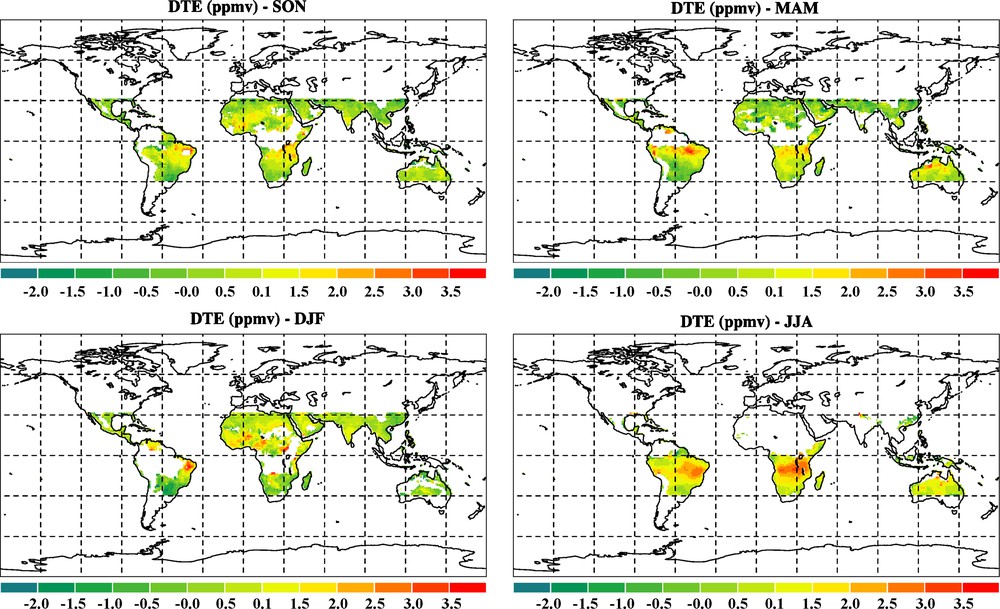
Daily Tropospheric Excess (DTE) derived from TOVS measurements for the four seasons. DTE is the difference in CO2 concentration measured in the early evening and early morning in the high troposphere. It is interpreted as the result of dry convection associated to the fires that uplifts CO2-enriched air to the high atmosphere. This air is then evacuated during the night by strong winds. Images provided by Alain Chédin, Laboratoire de météorologie dynamique.
Daily Tropospheric Excess (DTE) déduit des mesures de l’instrument TOVS pour les quatre saisons. DTE est la différence de concentration de CO2 déduit des mesures du soir et du matin. Le signal le plus fort est observé dans les zones et pour les saisons où se produisent des feux importants, essentiellement associés à une activité agricole. L’air enrichi en CO2 est transporté à haute altitude par la convection sèche forcée par les feux, puis évacué pendant la nuit par les forts vents de haute altitude. Figures fournies par Alain Chédin, Laboratoire de météorologie dynamique.
In summary, it is now clear that TOVS measurements cannot be used to infer sources and sinks of CO2. It is still debated on whether the TOVS observations can provide quantitative information for carbon cycle studies, in particular for biomass burning activity.
4.2 AIRS and IASI
The AIRS instrument is the first high-spectral-resolution infrared sounder developed by NASA in support of operational weather forecasting by the National Oceanic and Atmospheric Administration (NOAA). It was launched onboard the AQUA platform on May 4, 2002.
The heart of the instrument is a cooled (155 K) array grating spectrometer operating over the range of 3.7–15.4 μm at a spectral resolution (λ/Δλ) of 1200. The instrument concept requires no moving parts for spectral encoding and provides 2378 spectral samples, all measured simultaneously in time and space. AIRS views the ground through a cross track rotary scan mirror which provides ± 49.5° ground coverage along with views to on board spectral and radiometric calibration sources every 2.67 s scan cycle. The AIRS IR spatial resolution is 13.5 km from the nominal 705.3 km orbit.
AIRS provides daily near-global coverage both day and night. The primary objective of AIRS is meteorology with the retrieval of temperature and water vapour profiles. The goal for temperature profiles is a vertical resolution of 1 km and an accuracy of 1 K RMS. Water vapour profiles are expected with a resolution of 3 to 5%. These numbers apply to clear scene or significantly above the cloud layer.
In addition to using the AIRS data to generate relatively well established “core products”, i.e., temperature and moisture vertical profiles, surface temperature, and total column ozone, members of the AIRS science team are also working on a number of products where feasibility, achievable accuracy, precision, spatial and temporal coverage are not fully established. Products under development include carbon dioxide total column and methane concentration.
In the past year there have been several studies to assess whether AIRS measurements could be used to estimate the concentration of carbon dioxide (Chédin et al., 2003a; Engelen and Stephens, 2004). As said above, the primary variable that controls the radiance measured by the satellite is the temperature. Atmospheric CO2 concentration does have an effect, but this effect is relatively small when accounting for the typical variability of both temperature and CO2 concentration. Nevertheless, radiative transfer simulations studies indicate that some useful CO2 signature may be obtained by combining the measurement of channels that peak at similar levels in the atmosphere, but sensitive to the concentration of different gases (such as CO2 and oxygen). Because oxygen is a well-mixed gas, the relative concentration of CO2 can be estimated. The CO2 signal is still small with regards to the radiometer noise level so that considerable averaging may be needed to derive a useful concentration at the better than 1% level (Engelen and Stephens, 2004). Moreover, the radiative transfer simulations clearly indicate that the method is sensitive to concentrations above about 700 hPa. There is no sensitivity to the atmospheric boundary layer.
Strow and Hannon (2008) have confirmed that the increase of CO2 mixing ratio in the atmosphere has a measurable effect on the globally averaged AIRS temperatures. Initial attempts to retrieve CO2 monthly products from AIRS data followed the same approach as with TOVS, i.e., a neural network applied on carefully selected channels (Crevoisier et al., 2004). The retrievals were limited to the tropics for the same reason as given for TOVS above. Although the global CO2 distributions appeared reasonable, it was rapidly realized that the retrieved spatial features were not solely due to CO2 and that very significant biases affected the retrievals.
A group at ECMWF assimilated the AIRS radiance in the operational weather forecast system to retrieve the CO2 mixing ratio of the upper troposphere (Engelen et al., 2009). The initial results were limited to the tropical zone, and the monthly mean random error was estimated to be 1%. The first comparison against results from several models (constrained by surface observations of CO2) show model-observed differences that are larger than model–model differences, together with very intriguing feature in the observations (Tiwari et al., 2006).
Another group attempted another method to retrieve CO2 from AIRS (Chahine et al., 2005). It was shown that the retrieved CO2 seasonal cycle was in agreement with the result of aircraft observation, although with significant noise. The same group produced global maps of retrieved CO2 that differed significantly from those derived from best knowledge of surface flux and atmospheric transport models (Chahine et al., 2008) (Fig. 3). These differences were attributed to error in the atmospheric transport simulation. At present, consensus in the community is rather that biases remain in the retrieval, in particular due to undetected clouds.
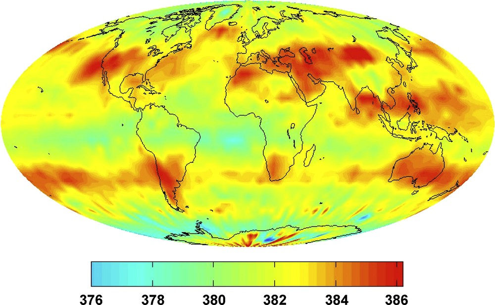
Upper troposphere estimate of CO2 mixing ratio derived from measurements of the AIRS instrument onboard the NASA-Aqua spacecraft. These estimates are provided by a NASA team at the Jet Propulsion Laboratory, led by M. Chahine. This image is an average for July 2008. The interpretation of spatial structures or this image, and other similar ones obtained from the AIRS measurements, is still debated in the scientific community.
Distribution spatiale de la concentration du CO2 atmosphérique dans la haute troposphère, déduite des mesures de l’instrument AIRS à bord du satellite Aqua de la NASA. Ces estimations ont été faites par une équipe NASA au Jet Propulsion Laboratory, dirigée par M. Chahine. Cette carte est une moyenne pour le mois de Juillet 2008. L’interprétation des gradients obtenus à partir des mesures AIRS fait encore débat dans la communauté.
There is a large choice in the selection of the AIRS channels that may be used to estimate the CO2 weighted column. All choices that have been proposed so far lead to a sensitivity limited to the upper troposphere. However, Strow and Hannon (2008) suggested a combination of channels that led to a sensitivity lower in the atmosphere, with a limitation to oceanic sampling for a lower variability of surface emissivity. The analysis was performed over large ocean basins or zonal means and demonstrated an accuracy close to 1 ppm at this scale. Spatial averaging is needed to get a sufficient number of clear observations and to statistically decrease the noise in the retrievals.
The IASI instrument has been launched by ESA on the Metop platform. It provides high spectral resolution in the thermal infrared, similar to that of AIRS, and also shares with this instrument the main objective of estimating temperature and water vapor profiles for weather forecast purposes. Similarly to AIRS, it may also be used for climate purposes and for the estimate of atmospheric compositions. There is no reason to believe, however, that IASI can do much better than AIRS. To our knowledge, there has not been any successful attempt for the estimate of carbon dioxide or methane from IASI measurements.
In summary, one shall recall that the AIRS instrument was launched more than 7 years ago with a focus on temperature retrievals. There have been several attempts at estimating CO2 from its measurements by groups in Europe and the US. Although it has been demonstrated that there is a CO2 signal in the data, the errors in the retrieval are still too large to provide novel information on surface CO2 fluxes (Chevallier et al., 2005). This disappointing result derives from the relatively high weighting function of the retrievals. In the upper troposphere, the CO2 signal is dominated by the seasonal cycle and excursions around this cycle are limited to one or a few ppm. To provide useful information, the accuracy requirements are then even stronger than for an instrument that is sensitive to the low atmospheric levels. Such requirements have not yet been met and it is not clear whether they can be met. In addition, the retrievals appear to be affected by regional biases, which have a devastating effect on the estimates of surface fluxes. It is likely that retrievals of CO2 from thermal infrared instruments such as AIRS or IASI will mostly be used to identify errors in the transport models rather than be used to constrain sources and sinks.
4.3 SCIAMACHY
The SCIAMACHY instrument was launched onboard the Envisat spacecraft on 28th February 2002. Scanning Imaging Absorption Spectrometer for Atmospheric Chartography (SCIAMACHY) is a spectrometer designed to measure sunlight, transmitted, reflected and scattered by the earth atmosphere or surface in the ultraviolet, visible and near infrared wavelength region (240–2380 nm) at moderate spectral resolution (0.2–1.5 nm). The absorption, reflection and scattering characteristics of the atmosphere are determined by measuring the extraterrestrial solar irradiance and the upwelling radiance observed in different viewing geometries.
SCIAMACHY has several modes of operation: Nadir, Limb, and occultation. In Nadir mode the atmospheric volume under the spacecraft and across-track is observed. Each scan covers an area on the ground of up to 960 km across track with a maximum resolution of 26 km × 15 km, albeit with resolution of typically 30 × 60 km for the channels sensitive to greenhouse gases. In Limb mode the instrument looks at the edge of the atmosphere. One novel characteristics of SCIAMACHY is the possibility to observe the same atmospheric volume first in limb and then, after about 7 min, in nadir geometry. In practice, however, no result concerning CO2 and exploiting either the dual-view or the occultation technique has been published. On the other hand, there are many ongoing studies and published results that use the “nadir” mode of SCIAMACHY to estimate atmospheric concentration of CO2 and CH4. These are discussed below.
Due to its near-infrared nadir observation capability, SCIAMACHY is the first satellite instrument that is sensitive to CO2 in the boundary layer where most variation occurs (Buchwitz et al., 2005). Therefore, SCIAMACHY CO2 retrievals play a pioneering role and required the development of dedicated retrieval algorithms. The retrieval schemes adjust the measured radiance around 1.6 μm to the result of radiative transfer simulations, accounting for a number of atmospheric and surface parameters. The CO2 mixing ratio that is retrieved is an averaged over the full column, with a weighting function that is close to 1 throughout the vertical profile. Note however that the measured spectra are sensitive, not so much to the CO2 mixing ratio, but rather to the CO2 column (in terms of mass or number of molecules). To derive a mixing ratio, it is therefore necessary to normalize the column using either the simultaneously measured O2 column (using the A band at 765 nm) or a knowledge of the surface pressure derived from numerical weather analysis.
First attempts at deriving the CO2 column from SCIAMACHY showed the possibility to observe the hemispheric gradient of atmospheric CO2 (Buchwitz et al., 2005), although not with the expected accuracy. These first analyses rapidly showed the strong impact of atmospheric aerosols (Aben et al., 2007; Houweling et al., 2005). Several groups have taken up the challenge however, and the quality of SCIAMACHY retrievals has been significantly improved (Barkley et al., 2006a). This was due in part to a better understanding of the radiometer systematic measurement errors (Buchwitz et al., 2006) and to the use of accurate temperature profiles in the inversion process.
The global average concentration derived from SCIAMACHY is in reasonable agreement with the same quantity constrained by surface observations (Buchwitz et al., 2007). Near-global monthly maps of CO2 column concentration have been derived from SCIAMACHY and have been compared to AIRS results (Barkley et al., 2006a), modelling results (Barkley et al., 2006b; Schneising et al., 2008) or column measurements provided by a sun-looking FTIR (Barkley et al., 2006b; Buchwitz et al., 2006; Schneising et al., 2008). In general, there is a good correlation between the satellite measurements and the validation products. There is also a rather large scatter of up to 10 ppm. Besides, the seasonal cycle of the satellite product in the Northern Hemisphere appears significantly larger than what can be expected from the numerous surface observations and a few airborne profiles (Barkley et al., 2006b; Buchwitz et al., 2007). There is currently a controversy in the carbon cycle community on whether the unexpected CO2 features monitored by SCIAMACHY are real or the result of a bias in the data processing. At present, the data appears too different from the modelling outputs to be used in an inversion scheme for the retrieval of CO2 surface fluxes. Nevertheless, SCIAMACHY was seen as a great tool to validate the OCO/GOSAT concept and to prepare the processing and analysis of these missions (Bosch et al., 2006).
The challenge of methane retrievals is somewhat easier as the spatial and temporal gradients generated by surface sources are, relative to the background concentration, larger than for CO2. Similar techniques as those described above have been applied and maps of column CH4 estimates have been produced, an example of which is shown in Fig. 4. The initial results have shown tropical concentrations much larger than expected (Frankenberg et al., 2005) which was tentatively explained by a yet unidentified source of methane produced by plants (Houweling et al., 2006). It was soon found, however, that the large tropical CH4 excess was due to inaccuracies in the spectroscopic database used to interpret the measurements in terms of concentrations (Frankenberg et al., 2008). Despite the corrections, the CH4 concentration maps are still rather different than those expected from the current knowledge of methane sources, chemistry and transport modelling (Meirink et al., 2008). It is still not clear whether this results from retrieval errors or from misunderstanding in the cycle of methane that could be resolved using remotely sensed data. Comparison with atmospheric transport simulations has shown biases in the retrievals, but also the potential of the product to identify large sources (Bergamaschi et al., 2007).
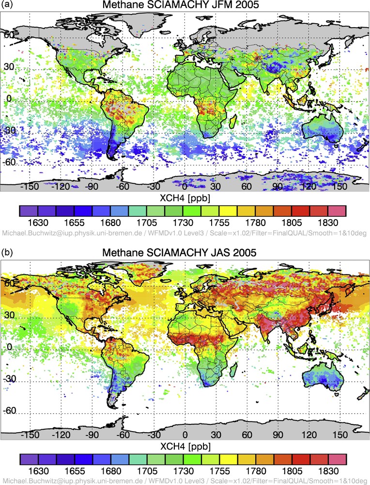
Global maps of column CH4 mixing ratio retrieved from SCIAMACHY during year 2005. Two extreme seasons for the CH4 seasonal cycle are shown, JFM (upper) and JAS (lower). The retrievals require a high sun, which explains the difference in coverage between the two seasons. Note the higher concentration in the Northern Hemisphere than in the south, and the high concentrations in regions with biomass burning activity and anthropogenic emissions. Images provided by Michael Buchwitz, University of Bremen, Germany.
Cartes montrant la distribution spatiale de la colonne de méthane déduite des mesures de SCIAMACHY pour deux saisons, JFM (haut) et JAS (bas). L’estimation nécessite un soleil suffisamment élevé, ce qui explique la différence de couverture entre les deux saisons. Ces cartes ont été réalisées et mises à disposition par Michael Buchwitz, Université de Bremen, Allemagne.
Note also that SCIAMACHY, even with continuous improvements in the data processing, will always have important limitations for the monitoring of CO2 or CH4 from space. One is due to the very large size of the field of view, so that most observations are cloud contaminated. Another arises from its spectral resolution that is insufficient to identify individual absorption lines. Finally, the viewing geometry is cross-track. This is well suited over land surfaces and actually provides better coverage than pure nadir instruments do. On the other hand, this geometry is rarely favourable over the oceans so that the monitoring of CO2 is, for the most part, limited to land areas. These limitations (FOV size, spectral resolution, viewing geometry) are corrected for the forthcoming CO2 dedicated missions.
In conclusion, the SCIAMACHY instrument allows a proof of concept for the monitoring of CO2 and CH4 from space using the differential absorption technique. The quality of the retrievals has been very much improved since the first versions of the processing algorithms and some features of the CO2 and CH4 spatial and temporal distributions can be measured. There is still no consensus on the value of SCIAMACHY data for an improved knowledge of CO2 and CH4 atmospheric concentrations, or to better constrain their surface fluxes. The instrument was not optimized for the monitoring of these gases and it is reasonable to expect significantly better results with the forthcoming missions that are dedicated to the monitoring of atmospheric concentration from space.
4.4 GOSAT
The GOSAT mission is developed as a cooperation between JAXA, the Japanese space agency and NIES, the National Institute for Environmental Studies. It is designed for the accurate measurement of CO2 and CH4 columns using the solar spectroscopy technique. GOSAT also carries a thermal infrared sensor, but the main products of the mission are expected from the Fourier Transform Spectrometer that operates in the solar spectrum. The satellite was launched in January 2009 and the first spectra acquired soon after. It is therefore the first satellite mission to be dedicated to greenhouse gases monitoring. At the time of writing, a few spectra and preliminary retrievals have been released. The spectra demonstrate that the instrument is functioning as anticipated. However, they are not yet properly calibrated. The CO2 or CH4 partial column are retrieved from the depth of their absorption lines in spectral bands around 1.6 and 2 μm while an oxygen absorption band at 0.76 μm is also used for reference and normalization: Since oxygen is a well-mixed gas in the atmosphere, the depth of the oxygen absorption lines in the spectra provides a reference indicative of the sunlight atmospheric path.
The instrument has the capability to point on specific targets, but the normal mode of operation is cross-track scanning with up to 9 samples perpendicular to the satellite subtrack. However, as the number of cross-track samples increases, the signal-to-noise decreases so that it may be necessary to limit the number of cross-track observations. In addition, there is a limitation over the oceans as water is dark at the wavelengths of interest, except in the glint direction. Only a fraction of GOSAT observations are acquired in the favourable “sunglint” viewing geometry. This geometry constrain will strongly limit the density of valid observations over the oceans.
At the time of writing, there is no product that can be used for an estimate of their accuracy. One has therefore to rely on theoretical estimates. The signal-to-noise estimates vary as a function of solar angle and surface albedo. They lead to errors that vary between 0.5 and 1% depending on the scene. The usefulness of GOSAT products to better constrain sources of CO2 and CH4 will depend on the error statistics. For CO2, there is a large difference in the potential impact of the product whether a 0.5% (≈ 1.5 ppm) or a 1% (≈ 3 ppm) accuracy is reached. In addition, the results will very much depend on the regional biases: A fully random error is acceptable as spatial and temporal averaging decreases its amplitude, while a regional bias of a fraction of a % may have a large impact on the flux distribution estimated. It will probably take several years to properly quantify the accuracy of GOSAT product and assess their usefulness for the carbon cycle community.
4.5 OCO
In the framework of the NASA ESSP program, the OCO mission was selected in July 2002. The launch occurred on 24 February 2009 but the rocket's payload fairing failed to separate properly, which prevented the satellite to reach orbit. The OCO instrument aimed at measuring carbon dioxide columns with the differential absorption technique, i.e., a technique similar to that of SCIAMACHY or GOSAT (Crisp et al., 2004; Connor et al., 2008). The stated accuracy objective was 1 ppm averaged concentration and numerical simulations indicated that an even better accuracy could be achieved in favourable conditions (Bosch et al., 2006; Connor et al., 2008). The instrument was designed to make very high spectral resolution measurements close to 1.6 μm and 2 μm, two spectral bands that show a few narrow CO2 absorption lines, and that are free from other gases absorption, and at 0.76 μm that corresponds to an oxygen absorption band. The latter is used for correction of surface pressure and atmospheric scattering. The viewing geometry mode of OCO was very innovative with three modes of operation: Nadir, glint and target. In the nadir mode, the instrument looks straight down. In the glint mode, the instrument follows the glint direction. This is necessary over the ocean to get a sizeable reflectance from the surface. Finally, the instrument may aim at specific targets. The later mode is designed for the calibration and validation of the CO2 products based on coincident observation with ground-based FTIR. In “nadir” mode, the measurement track is one-dimensional so that it seldom samples a ground truth point. The agile capability makes it possible to view a calibration site (target) almost everyday (weather permitting). The ground calibration and validation can partly be achieved through the measurement of a spectra derived from a Fourier Transform Interferometer (FTIR). At present, there is a global network of 10 ground based FTIR spectrometers (www.tccon.caltech.edu). These instruments were shown to accurately measure column CO2 and CH4 concentrations, when compared with aircraft vertical profiles on a campaign basis (Dufour et al., 2004; Washenfelder et al., 2006).
At the time or writing, there are discussions at NASA whether a copy of the original OCO mission should be built rapidly or whether it should focus on the next generation of CO2 monitoring instruments, based on the active technique.
4.6 A-SCOPE and ASCENDS
Two active missions have been proposed for the monitoring of CO2 from space. The A-SCOPE mission was considered by the European Space Agency in the Earth Explorer context, while Active Sensing of CO2 Emissions over Nights, Days, and Seasons (ASCENDS) is currently considered by NASA. The A-SCOPE concept was evaluated as too demanding for a launch in 2016 so that it did not pass the next round of selection that took place in January 2009. On the other hand, an airborne version of the ASCENDS concept has been built. The flights that took place confirm the potential concept and the theoretical considerations that ASCENDS meets the science requirement of 0.5% precision measurement of CO2 mixing ratio along a 100 km horizontal segment. Nevertheless, it is clear that the active mission is much more demanding than a passive one. Besides, the accuracy of the CO2 column estimates is not necessarily better than that of the passive missions using the differential absorption technique.
5 Conclusions
There are both scientific and societal needs for a better understanding of the carbon cycle and its impact on the atmospheric composition. A key element for this understanding is the monitoring of carbon dioxide and methane fluxes at regional scales. This can be achieved through the inversion of atmospheric transport using constrains provided by accurate measurements of concentration gradients in the atmosphere. The current in situ network allows to estimate fluxes at continental scales, but it is clearly insufficient to resolve finer regional scale. In this context, a satellite monitoring of the atmospheric concentration is very appealing. This need has been recognized by the scientific community and by space agencies.
Several instruments, already in flight, were not specifically designed to measure CO2 and CH4. Nevertheless, responding from a pressing demand, several teams have taken up the challenge of using their measurements to retrieve column concentrations of these gases. Since the first attempts in 2002, considerable progress has been made. Accuracy and biases remain a challenge, however. The spatial and temporal concentration distributions that are retrieved do show some of the expected features such as the annual growth rate, the seasonal cycle and the latitudinal gradient. However, additional knowledge on the carbon cycle requires the identification of gradients of smaller magnitude. The biases and noise in current satellite products are still larger than these gradients amplitude. As a consequence, the assimilation of such data in atmospheric transport models brings little new information to our current knowledge of the surface fluxes (Fig. 5).
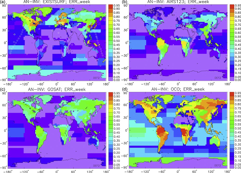
Error Reduction on the surface CO2 fluxes that may be expected from the use of various observing systems through atmospheric transport inversion. The globe is subdivided into 200 regions, whose contours can be depicted on the figures. A perfect knowledge of surface fluxes corresponds to a value of unity, whereas no additional knowledge from the first guess corresponds to a value of zero. From left to right and top to bottom: The existing surface network of about 100 stations, the AIRS instrument onboard the Aqua satellite, the JAXA/GOSAT mission, and the NASA/OCO mission. These results have been obtained at the Laboratoire des sciences du climat et de l’environnement, in the context of a study funded by the European Space Agency using the LMDz atmospheric transport model.
Réduction d’erreur sur notre connaissance actuelle des flux de surface de CO2, qui peut être attendue de l’utilisation de systèmes de mesures de la concentration atmosphérique par une technique d’inversion du transport atmosphérique. Le globe a été subdivisé en plusieurs régions, dont on peut distinguer les contours. Une valeur de 1 correspond à une connaissance parfaite des flux, alors qu’une valeur de zéro n’indique aucune information supplémentaire par rapport à l’a priori. Les systèmes d’observation dont les résultats sont montrés ici sont, de gauche à droite et de haut en bas : le réseau de prélèvement de surface, l’instrument AIRS à bord du satellite Aqua, la mission GOSAT de la JAXA, et la mission OCO de la Nasa. Ces résultats ont été obtenus avec le modèle de transport LMDz dans le cadre d’une étude financée par l’Agence spatiale européenne.
The first dedicated instrument, GOSAT, was launched recently and the first column CO2 data are expected during 2009. This instrument uses the differential absorption technique, allowing the sampling of the low atmospheric layers, which are directly connected to the surface fluxes. Accuracy of the column concentration estimates will be a key element in the success of the mission. Indeed, a significant improvement on our current knowledge of the possible surface will only be possible if the accuracy of individual estimates is significantly better than one percent, while the requirement on regional biases is even stronger. There are few remotely sensed parameters that are retrieved with that level of accuracy.
Acknowledgments
We thank M. Chahine (NASA-JPL), A. Chédin (IPSL/LMD), M. Buchwitz, (Univ. Bremen), K. Hungeshoefer (IPSL/LSCE) for providing some of the figures shown in the paper.