Assimilation of satellite observations of the atmosphere

Paul Poli

doi:10.1016/j.crte.2009.10.014

External geophysics, climate and environment (Aeronomy and meteorology)

Assimilation of satellite observations of the atmosphere
[Assimilation des observations de l’atmosphère par satellite]

Présenté par : Written on invitation of the Editorial Board

Paul Poli ¹

¹ European Centre for Medium-range Weather Forecasts, Shinfield Park, Reading RG2 9AX, United Kingdom

Comptes Rendus. Géoscience, Volume 342 (2010) no. 4-5, pp. 357-369.

Résumés

Anglais
Français

Measurements of the atmosphere by satellite were first collected in the 1960s. However, it was not until the mid-1990s that these observations were translated into systematic improvements of numerical weather forecasts. We present here the data and methodology of data assimilation that enabled this achievement. Data assimilation is essentially a filtering processing that exploits the (assumed) known error statistical properties of the observations and of the underlying numerical model in which data are assimilated. It is also a process which corrects the state of the numerical model with physical observations of the real world. This part relies on (assumed) known physical laws to relate meteorological quantities (such as temperature, humidity, pressure, and wind) to observables. Atmospheric data collected by satellite all come from the interaction of electromagnetic waves with the atmosphere. Satellite data assimilation has greatly supported the progress in numerical weather prediction and holds promises for climate studies, for example via reanalysis.

Les premières mesures de l’atmosphère par satellite remontent aux années 1960. Cependant, ce n’est que depuis le milieu des années 1990 que ces observations se sont traduites par des améliorations systématiques dans les prévisions numériques du temps. Cet article présente les données et les méthodes d’assimilation de données qui ont permis d’arriver à ce résultat. L’assimilation de données est essentiellement un filtre qui exploite les propriétés (supposées) connues des erreurs des observations et du modèle numérique dans lequel ces observations sont assimilées. L’assimilation est aussi un processus qui contraint le modèle numérique à reproduire les observations physiques du monde réel. Cette partie repose sur des lois physiques (supposées) connues reliant les différents paramètres météorologiques (tels que température, humidité, pression et vent) aux observables. Les données météorologiques collectées par les satellites résultent toutes de l’exploitation d’interactions entre l’atmosphère et les ondes électromagnétiques. L’assimilation des données satellite a beaucoup contribué aux progrès en prévision numérique du temps et pourrait contribuer de manière significative aux études sur le changement climatique, par exemple via la réanalyse.

Métadonnées

Reçu le : 2009-08-17
Accepté le : 2009-10-26
Publié le : 2010-01-06

DOI : 10.1016/j.crte.2009.10.014

Keywords: Atmospheric spectrum, Earth system modeling, Kalman filtering, 3DVAR and 4DVAR, Multi-disciplinarity, Refraction
Mot clés : Spectre atmosphérique, Modélisation du système Terre, Filtre de Kalman, 3DVAR et 4DVAR, Multidisciplinarité, Réfraction

Affiliations des auteurs :

Paul Poli ¹

¹ European Centre for Medium-range Weather Forecasts, Shinfield Park, Reading RG2 9AX, United Kingdom

@article{CRGEOS_2010__342_4-5_357_0,
     author = {Paul Poli},
     title = {Assimilation of satellite observations of the atmosphere},
     journal = {Comptes Rendus. G\'eoscience},
     pages = {357--369},
     publisher = {Elsevier},
     volume = {342},
     number = {4-5},
     year = {2010},
     doi = {10.1016/j.crte.2009.10.014},
     language = {en},
}

TY  - JOUR
AU  - Paul Poli
TI  - Assimilation of satellite observations of the atmosphere
JO  - Comptes Rendus. Géoscience
PY  - 2010
SP  - 357
EP  - 369
VL  - 342
IS  - 4-5
PB  - Elsevier
DO  - 10.1016/j.crte.2009.10.014
LA  - en
ID  - CRGEOS_2010__342_4-5_357_0
ER  -

%0 Journal Article
%A Paul Poli
%T Assimilation of satellite observations of the atmosphere
%J Comptes Rendus. Géoscience
%D 2010
%P 357-369
%V 342
%N 4-5
%I Elsevier
%R 10.1016/j.crte.2009.10.014
%G en
%F CRGEOS_2010__342_4-5_357_0

Paul Poli. Assimilation of satellite observations of the atmosphere. Comptes Rendus. Géoscience, Volume 342 (2010) no. 4-5, pp. 357-369. doi : 10.1016/j.crte.2009.10.014. https://comptes-rendus.academie-sciences.fr/geoscience/articles/10.1016/j.crte.2009.10.014/

Version originale du texte intégral

1 Introduction

The first measurements of the atmosphere from space were collected in the 1960s. The potential of these data for observing the atmosphere and improving weather forecasts was recognized immediately. The first television images confirmed the atmospheric general circulation theories. The collected imagery was also rapidly used daily by human forecasters to adjust the timing and location of synoptic forecasts obtained by other means, and increasingly by numerical forecasting. In the early 1990s, the quantitative impact of satellite data on numerical weather prediction was still unclear (Smith, 1991). It was not until the mid 1990s that this impact was fully realized. This happening owed heavily to the advent of data assimilation techniques capable of extracting automatically information from the satellite measurements to perform weather analyses.

The need for creating weather analyses became obvious in the early days of Numerical Weather Prediction (NWP) when observations had to be digitized onto model grids in order to provide initial conditions to a deterministic prediction model integration. The analysis subsequently evolved from a simple interpolation from observations to a more complex process called data assimilation where observations are blend or merged with an a priori (or background) estimate of the atmosphere. In this process, observation and background errors are taken into account to separate noise from signal. Models of the atmospheric circulation and of the observation process provide physical constraints so as to ensure a physically consistent representation of the atmosphere as a result.

The science of data assimilation sits at the intersection of applied mathematics and physics. Depending on one's background, data assimilation may be seen slightly differently. It is a mathematical filtering process, by which one separates signal from noise, assuming that the signature (or properties) of that noise is (are) properly known. It is also a process, by which one forces a model to reproduce physical observations. Both approaches are right if taken together, but can lead to suboptimal results if considered in shear ignorance of each other.

Data assimilation represents now a research field of its own. The reader is invited to consult the following sources for more information: Refs. (Daley, 1991) and (Kalnay, 2003), the proceedings of the WMO International Symposia on Assimilation of Observations in Meteorology and Oceanography (for example, Ref. (Ghil et al., 1997) and the special issue of the Quarterly Journal of the Royal Meteorological Society, vol. 131, no. 613, 2005), and the proceedings of the Adjoint Workshops (for example, see the special issue of Meteorologische Zeitschrift, vol. 16, no. 6, 2007). In the present paper, we take the angle of summarizing what satellite data assimilation is about, what has made its success, what its impact is, and what challenges lie ahead. Furthermore, efforts have been made to separate the particular aspects of meteorological satellite data assimilation from the general problem of data assimilation. This separation should be of interest to the general reader, not necessarily interested in meteorology. The particularity of meteorology is that the modeling capabilities today allow good propagation of information in time; as a result, meteorological data assimilation focuses on improving, with the help of observations, an initial estimate provided by a model forecast.

As a brief introduction to the problem, as of 2008, operational NWP (simply written NWP in the rest of this article) global models are routinely fed with about 19 million observations per day. Less than 1 million of these observations come from so-called conventional measurements. More than half of these conventional data come from aircraft, while the in situ surface and radiosonde observations only represent a fraction of the total. The bulk of the observations (about 18 million) are raw or more or less processed forms of measurements collected by satellite-borne instruments. Keeping such operations in a timely, efficient, and smooth fashion represents significant costs for the organizations that run them, from getting the data processed in time to meteorological centers to the assimilation. As will be shown in this paper, this comes to great, clearly proven, benefits through data assimilation.

The present article is organized as follows. Section 2 is a brief primer on the first application of satellite data assimilation: NWP modeling. Sections 3 and 4 present (respectively) the physical and statistical considerations in data assimilation methodology. Sections 5 and 6 present the implementation and the impact of data assimilation in NWP today. Section 7 contains a discussion on the future challenges and Section 8 presents concluding remarks.

2 Numerical models of the atmosphere

In Bjerknes’ 1904 visionary paper (Bjerknes, 1904), weather prediction was introduced as an initial-boundary problem to be solved with a deterministic numerical model. This justified the effort to collect atmospheric observations in order to improve subsequent weather forecast. Data assimilation in meteorology emerged from this need to apply the observations to initialize deterministic numerical models. Richardson, 1922 envisioned that numerical forecasts would be initialized with maps obtained by hand-performed interpolations from man-made observations. With the advent of the first computers, it became quickly obvious that this process as well should be automated (Charney, 1951). It is hence useful to first present the concepts relevant to the application which first drove the need for data assimilation in meteorology.

We denote M_i a deterministic model built to propagate the information describing the atmosphere at some time t_i to a later time t_i+1. The information handled by that model (i.e., the representation of the atmosphere at a time t_i) is described in a so-called state vector, noted x(t_i). Because that vector controls the state of the system, it is said to be in control variable space. The control variable space encompasses different physical variables discretized spatially.

2.1 State vector

The physical variables in the state vector include at least the surface pressure, the temperature, the water vapor content, and the wind, or an equivalent set of variables. The wind vertical component is not explicitly represented in the state vectors of models that assume hydrostatic equilibrium. This assumption, common in global models, is valid to describe horizontal scales larger than 5–10 km.

Chemically reactive constituents are also becoming represented in model state vectors. One such example is the ozone, whose large variability strongly influences the radiative equilibrium in the stratosphere. Aerosol size distributions are also typically not fully modeled but assumed to follow climatology. Like for chemical constituents, aerosols are coming under focus and may soon be part of meteorological model state vectors. Finally, the prognostic variables in today's atmospheric prediction models also typically include cloud liquid water, rain, cloud ice, snow, and graupel (supercooled water that condenses on snow). However, these variables are not yet routinely included in the state vector for analysis (this is still an ongoing research topic).

The deterministic model also requires additional information on boundary conditions at the top and at the bottom of the atmosphere (e.g., land, sea, sea-ice). Limited-area models further need lateral boundary conditions. Most of these conditions do not belong in the state vector because they are either invariant, or provided as a forcing, or considered to be unaffected by the deterministic atmospheric model during the integration time.

The numerical discretization of the physical variables horizontally and vertically depends on the target application of the prediction scheme. A common choice is a regular grid in physical space (latitude and longitude, or more complex). Global models may rely on a basis of spherical harmonics, owing to the near-spherical shape of the Earth. Limited-area models may instead be described in spectral space (by wavenumber). The vertical discretization reverts to either fixed-pressure levels, or sigma- or eta-levels (terrain-following formulations).

Operational global models today achieve horizontal resolutions that are on the order of 50 km with up to about 100 levels in the vertical. Operational limited-area models attempt to describe scale as small as 1–2 km but over smaller domains (surface areas of a few million km² maximum).

Consequently, depending on the model's resolution and the total number of prognostic variables, the size of x in today's global NWP models is close to 10⁷–10⁹. All these elements must be specified every time a new forecast is carried out.

2.2 Forecast cycle and forecast error growth

Lorenz, 1963 demonstrated the existence of limits to atmospheric predictability with a simplified convection scheme (known as the Lorenz attractor, whose solutions in phase space look like the wings of a butterfly). In his example, Lorenz observed that small errors in the initial conditions could grow exponentially very rapidly. In the most general case, the forecast error grows also because of errors in the model. Consequently, even if the initial conditions (model state x) were to be known perfectly at some time t_i (so-called truth, noted x^t(t_i)), the subsequent state of the model (x(t_i+1)) could not be known properly because the deterministic forecast model (M_i) is not perfect and generates errors (η(t_i), called model error, in data assimilation) as compared to the true evolution of the atmosphere:

x^{t} (t_{i + 1}) = M_{i} [x^{t} (t_{i})] + η (t_{i})

(1)

This justifies further the need to bring in observations regularly, in order to reduce the errors on the latest available estimate and obtain an analysis (noted x^a(t_i)) that will instead be used as the initial condition for the next forecast:

x^{a} (t_{i}) = G_{i} [x^{f} (t_{i}), y_{i}^{0}]

(2)

x^{f} (t_{i + 1}) = M_{i} [x^{a} (t_{i})]

(3)

where G_i denotes the data assimilation process that combines all the observations available at time t_i (noted y⁰_i). Consequently, the approach of bringing in observations in order to determine initial conditions attempts to solve for two distinct problems at the same time: an unknown atmospheric state at a given time, and an imperfect numerical weather model. As will be seen below, only the first problem has been addressed operationally so far. Although theoretical solutions exist for the second problem (e.g., Kalman filter, Kalman, 1960), their practical implementations are still lagging behind.

The time period of the cycle above (Eqs. (2) and (3), i.e., data assimilation and forecast) is application-dependent. It varies from 6–12 hours for global models to 1–3 hours for non-hydrostatic limited-area meso-scale models whose focus includes the prediction of severe weather events that tend to develop rapidly.

The pace of increase in model state vector size (related to refined model resolution) follows that allowed by the increase in computing power at a fixed price (dubbed Moore's Law). Although the forecast (background) reflects information extracted from past observations, the only external source of information at every analysis cycle is brought by actual observations. So there is a need to ensure that increasingly finer scales in the model can be corrected by increasingly finer-scale observations. Fortunately, the number of satellite observations increases over time with new satellite launches involving instruments increasingly complex and accurate (refined imaging resolution for example). These improvements in data acquisition and processing are also to some extent allowed by Moore's Law. So, at least until Moore's Law breaks down per lack of industry funding or fundamental technological changes, one can expect parallel growth in the number of observations collected daily and the number of state vector elements that need daily updating.

In the rest of the paper, an attempt has been made to separate the physical and statistical considerations in data assimilation, starting with the physical aspects.

3 Physical considerations in data assimilation methodology: observation operators

We initially restrict our discussion to the simple, linear form of sequential data assimilation (an extension to weakly non-linear cases is discussed later). The analysis vector state at time t_i (x^a(t_i)) is updated sequentially as the sum of a previous estimate valid at the same time (called background, noted x^b(t_i)) and a correction which scales linearly as the departure between the observation vector (y⁰_i) and the projection of the state vector in observation space (H_i[x^f(t_i)]):

x^{a} (t_{i}) = x^{b} (t_{i}) + K_{i} \cdot (y_{i}^{0} - H_{i} [x^{b} (t_{i})])

(4)

In meteorology, the background vector x^b(t_i) may simply be the forecast x^f(t_i), or the result of a reversible transform operation applied to x^f(t_i). For simplicity, we will assume here the former, so that x^b(t_i) = x^f(t_i).

The scaling factor K_i above is known as the Kalman gain matrix and will be described hereafter. It is based on physical and statistical properties of the observations and the background. We first focus our discussion on the description of the projection operator H_i, called observation (or forward) operator. This is also referred to as the direct problem in remote sensing jargon (Stephens, 1994). This operator relates the estimation problem to the measurement physical process.

The observation operator is observation-dependent: it depends on observation meta-data, such as data location, time, geometry, and observable type. At the very least, the observation operator involves an interpolation of a few variables from the state vector to the observation location. The observation operator can also incorporate a model to simulate the observation physics, which is particular to each observation type. The following discussion attempts to separate between the measurement and the inversion processes on the one hand, and the simulation process achieved by the corresponding observation (or forward) operator on the other hand.

All satellite measurements of the atmosphere today result, in one form or another, from the interaction of electromagnetic (EM) fields with the atmosphere. Consequently, observation operators for satellite data assimilation incorporate, in one form or another, models of EM wave propagation (and interaction) in (and with) the atmosphere.

To separate between the various types of observation operators, we consider here the four basic forms of EM/medium interactions: absorption and emission (related by Kirchoff's Law of radiation), scattering, refraction, and diffraction. We actually leave out the fourth form of interaction given that there is no generalized satellite remote sensing of the atmosphere that makes use of that interaction alone. However, as will be seen below, that interaction can play a role in the other interactions.

The first form of interaction, absorption and emission, helps collect most of today's satellite measurements. This technique relies on the measurement of the intensity collected in a given bandwidth of the EM spectrum either by the observation of an obvious source (sun or stars) through extinction by absorption by the atmosphere or by the observation of the (passive) radiation emitted by the atmosphere (emission). The raw measurements (radiances) are then the result of photon counting. Ideally, this process only counts the photons that arrive directly from the atmosphere into the instrument telescope and that feature a wavelength in a certain range. In practice, as in every experimental apparatus, the instrument can interact with its direct environment (e.g., other instruments on-board the satellite or the satellite itself) so that it is difficult to determine before flight the corresponding contamination of the signal reaching the instrument. The calibration of the detectors in amplitude (photon counting) and in frequency (or wavelength) is then of prime importance. This is achieved at processing level using models determined before flight and refined in the early days of the mission thanks to observation campaigns and cross-comparison with other observations (such as in situ measurements). The final observables derived afterwards are considered to be properly calibrated using possibly data collected on-board the spacecraft to keep track of calibration changes. The ramifications of the calibration aspect for long-term measurement stability are now being investigated by various groups, and the drifts in instrument behavior are the subjects of active research (Grody et al., 2004).

The instruments may feature the ability to observe various bandwidths (channels), so that the wavelength ranges are chosen in regions of the EM spectrum for which the interactions with the atmosphere are stronger. These regions may be right in the middle of, or on the edge of, rotation or vibration lines of air molecules or its constituents in the infrared or in the microwave. All radiance measurements contain information on the atmospheric temperature. Those measurements sitting in absorption regions of specific constituents also contain information on the amount of these constituents in the atmosphere.

3.1 Infrared radiances

A subset of instruments operating in the thermal infrared (3–18 microns) is shown in Fig. 1. The first example presented here is the Vertical Temperature Profile Radiometer (VTPR) which flew on the early National Oceanic and Atmospheric Administration (NOAA) polar-orbiting satellite series. The figure shows the typical brightness temperature that would be observed for mid-latitude conditions for all VTPR channels, with an indication of the molecules sensed by spectral region. Note that water vapor lines are all over the spectrum in the thermal infrared region, so only a selection of H₂O lines appears in the figure. The figure also shows the vertical region (in pressure levels) from which most of the signal originates. This is defined here as the region where the weighting function (vertical derivative of the transmittance) reaches its peak (see, for example, Ref. Smith et al., 1972). At the time the VTPR instruments were flown, the data collected were not assimilated by operational NWP as brightness temperature radiances, but as atmospheric retrievals: the observation operator simply consisted of an interpolation, while the retrieval process upstream of the assimilation consisted in a reconstruction of an atmospheric vertical profile.

Fig. 1
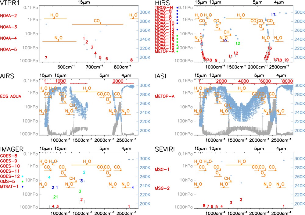
Selection of infrared radiometers whose data are or have been assimilated in NWP or in reanalyses. The satellites names are listed below the instrument names and the channels can be located by channel number (in red), wavelength, or wavenumber. Changes in channel positions between instruments from different generations are indicated by blue or green bullets next to the satellite name. Each plot shows for each channel the typical brightness temperature (right vertical axis) and the location in pressure level of the weigthing function peak (left vertical axis) for a mid-latitude atmospheric profile.
Sélection de radiomètres infra-rouge dont les données sont ou ont été assimilées en prévision numérique du temps ou dans des réanalyses. En dessous du nom de chaque instrument sont listés les noms des satellites sur lesquels une version de l’instrument a été embarquée. Les canaux peuvent être repérés, ou bien par numéro de canal (en rouge), ou bien par longueur d’ondes, ou bien par nombre d’ondes. Pour un instrument et un canal donnés, les éventuels changements dans la position spectrale du canal entre différentes générations de l’instrument sont indiqués par des points bleus ou verts à côté du nom du satellite affecté par le changement. Chaque figure montre, pour chaque canal, la température de brillance (axe vertical de droite) et le niveau pression où se situe le pic de la fonction poids (axe vertical de gauche), pour un profil atmosphérique représentatif des moyennes latitudes.

Later, on the same satellite series, came the High resolution Infrared Radiation Sounder (HIRS) and the Stratospheric Sounding Unit (SSU) as parts of the TIROS Operational Vertical Sounder (TOVS), featuring more channels covering the whole vertical range from the surface up to the 1 hPa pressure level, and enabling a better sounding of the atmosphere. With these instruments, the assimilation of passive infrared data moved to the direct assimilation of brightness temperature radiances. From then, the observation operator involved a more complete physical representation of the measurement process. At the same time, steps upstream of the assimilation were removed so that the assimilated data were closer to the raw measurement. The importance of this point will be discussed later on.

Other instruments shown in Fig. 1 are the Atmospheric InfraRed Sounder (AIRS) onboard the National Aeronautics and Space Administration (NASA) Earth Observing System (EOS) Aqua satellite and the Infrared Atmospheric Sounding Interferometer (IASI) onboard the Eumetsat Polar System operational satellite MetOp. These last two instruments feature several thousand channels with high spectral resolution, and are assimilated in NWP today. Note the overall increase in complexity between the generations of instruments: VTPR, HIRS, AIRS, IASI.

The major limitation of infrared measurements is that they interact with particulates of sizes close to the infrared wavelengths (i.e., clouds and aerosols). These complex interactions rely heavily on the characteristics of the clouds and aerosols, which are still largely un-observed with significant accuracy, resolution, and coverage, and hence, to a large extent, unknown on a systematic basis. It then becomes practically impossible to exploit all the cloud-affected measurements without significant modeling efforts, which are today out of reach of operational data assimilation schemes. Consequently, raw infrared measurements today are deemed useless in cloudy regions (except above the clouds) for assimilation purposes. This limits seriously the ability of infrared emission measurements to observe severe weather deep inside cloud formations. As a result, only the clear infrared data (less than 10% of the total) are assimilated. This limitation and the near-real time dissemination of only a subset of the channels from AIRS and IASI mean that the full potential of these instruments remains to be realized.

Fig. 1 also shows IR instruments on geostationary satellites: the Spinning Enhanced Visible and InfraRed Imager (SEVIRI) onboard Eumetsat Meteosat second-generation satellites and the imager onboard the NOAA Geostationary Operational Environmental Satellite (GOES) series. These data offer a high repeat frequency of observation for fixed locations.

The observation operators to simulate atmospheric infrared radiances are derived as follows. Line-by-line radiative transfer models are first applied to various types of simulated atmospheres discretized along the vertical. Each vertical slab of atmosphere emits monochromatic radiation (Planck's Law) that is then propagated in the vertical (Lambert's Law), taking into account the absorption of each successive slab between the emitting layer and the top of the atmosphere. Emission by the surface is also accounted for. The resulting spectral radiances are then convolved with the instrument/channel response function to obtain an equivalent modeled radiance for each instrument and channel. Because this approach is too slow for practical, repeated computations, fast radiative transfer models are then derived using sets of well-chosen predictors from these exact computations. Examples of such model are the Radiative Transfer model for TOVS (RTTOV, Saunders et al., 1999) and the Community Radiative Transfer Model (CRTM, Chen et al., 2008).

3.2 Microwave brightness temperatures

In a similar fashion, as for infrared measurements, brightness temperatures in the microwave region collect information on atmospheric temperature and constituents. Such observations from space are available, for example from the Advanced Microwave Sounding Unit-A and -B (AMSU-A, and -B, earlier satellites carried MSU), the Microwave Humidity Sounder (MHS), and the Defense Meteorological Satellite Program (DMSP) series carrying the Special Sensor Microwave Imager (SSM/I). From nadir geometry, the vertical resolution of these measurements is coarser than that of infrared measurements.

Though insensitive to clouds, microwave measurements can be affected by rain as the EM wavelengths under consideration get closer to the size of rain droplets. To circumvent this problem, one approach has been to perform retrievals before the assimilation so that the quantity to be assimilated is closer to the numerical model (for example, total precipitable water, Baüer et al., 2006). However, like for earlier infrared data, this intermediate step between measurement and assimilation comes to the cost of increased complexity in the error patterns of the assimilated data. Note that microwave data are especially sensitive to surface emissivity properties. Efforts are underway to benefit from these data over land (Karbou et al., 2006).

3.3 Atmospheric Motion Vectors from imagery

Another application of the first form of EM-atmosphere interaction is the derivation of atmospheric motion vectors (AMVs) from features tracked by satellite imagery. Originally, this technique was only applied from geostationary orbit because the geometry of the imagery remains nearly identical from one image to the next. But with recent improvements in computing power, it has become possible to apply a similar technique to images of the Polar Regions observed under different geometries by successive passes of polar-orbiting satellites. Examples include winds generated from GOES, Meteosat, and MTSAT (Japan) satellite imagery, as well as from the Moderate Resolution Imaging Spectroradiometer (MODIS) imagery collected by the NASA EOS Aqua and Terra satellites. The observation operator simply interpolates the model wind at the atmospheric motion vector location.

3.4 Scattering measurements

The second type of interaction is scattering (includes back-scattering). Except in situations of multiple scattering when photons can actually be added along a certain direction, scattering is usually associated with the removal of photons from radiation that is incident along the line-of-sight of the instrument (Beer's Law). The received intensity gives an indication on the (back) scattering coefficient.

The source of radiation may be either solar or man-made. In the latter case, the EM waves may be either in the radio range (radar) or in the near-infrared to ultraviolet (lidar). Also, the response time of an encoded signal can give an estimate of the distance of the target.

The interpretation of scattering measurements typically applies simplified results from molecular scattering (Rayleigh) or from aerosols scattering (Mie) theory, or from laboratory or campaign measurements to relate the backscatter coefficient to the target properties.

In the case of scattering measurements from space, the observation operator may simply interpolate from the state vector to assess the meteorological parameter as inferred by retrieval (for example, ozone or aerosol content) from the raw measurements.

Examples of scattering measurements are as follows. The Solar Back-scatter Ultra-Violet (SBUV) instruments onboard NOAA polar-orbiting satellites yield ozone content measurements. The Precipitation Radar (PR) onboard the Tropical Rainfall Measuring Mission (TRMM) and the Cloud Profiling Radar (CPR) onboard Cloudsat yield estimates of rain rates. Lidar backscatter measurements (e.g., Cloud Aerosol Lidar and Infrared Pathfinder Satellite Observations, CALIPSO) yield retrievals of aerosols contents. Also, although they do not remotely sense the atmospheric backscatter but the ocean surface backscatter, the European Remote Sensing satellite-1 and –2, the Seawinds instrument onbard the Quikscat satellite, and the Advanced scatterometer ASCAT onboard MetOp yield wind retrievals above the sea surface. Only the first and last examples (SBUV and ocean scatterometers) have matured to operational assimilation. Efforts are underway to start assimilating data from the other two examples, using a retrieval step before assimilation (Benedetti et al., 2005) or comparing the performance of today's atmospheric models with radar data (Marchand et al., 2009).

Another application of scattering measurements is to detect the motion of sensed particulates, by measuring the Doppler shift of the backscattered wave. The observation operator may then simply reproduce the projection of the wind along the line-of-the-sight of the instrument from the state vector wind information interpolated at the observation location. One example is the Atmospheric Dynamics Mission-Aeolus currently under development by the European Space Agency (Tan et al., 2008).

3.5 Refraction measurements

Astronomers and geodesists have so far always regarded the third type of interaction, refraction, as a source of error for locating the position of celestial stars. In meteorology, it has emerged lately as a robust source of observations.

The atmospheric refraction measurements assimilated today in NWP are collected thanks to the U.S. Global Positioning System (GPS). The EM waves carrying GPS signals undergo refraction as they propagate from their entry in the atmosphere to the receiver. The transmitters are orbiting at about 20000 km altitude while the receivers may be either on the ground (fixed stations) or in a satellite in orbit (GPS radio occultation, e.g., Kursinski et al., 1995). Note that in the latter application, as the scales of the gradients being sensed can sometimes be close to a few times the wavelength considered, phenomena of diffraction can appear. Their effect on the amplitude and phase data collected can be corrected by ad hoc algorithms.

The observation operator in both cases simulates first the radio refractive index from meteorological variables (temperature, pressure, water vapor). A second step reproduces the observation geometry and integrates this index or its vertical derivative in order to yield measurements of bending angle for GPS radio occultation and of Zenith Total Delay (ZTD) for ground-based GPS. Data collected by these methods have been assimilated in global NWP since 2006 (respectively: Healy et al., 2005; Poli et al., 2007).

4 Statistical considerations in Data Assimilation methodology: Kalman gain matrix

The Kalman gain matrix mentioned earlier is the cornerstone of data assimilation. This matrix controls the extraction of signal from (error-contaminated) observations in order to improve the (error-contaminated) background and form the analysis.

As an aside note, it is useful to remind that one of the first applications of the Kalman filter (Kalman, 1960) was trajectory determination, in the early days of the U.S. lunar exploration program. Since then, this algorithm has been applied to great benefits in other fields.

We now provide a few keys to help understand the origins of the Kalman gain matrix in atmospheric satellite data assimilation. Let us first assume that we are only given two observations T₁ and T₂ to estimate the state of a one-variable “toy system”. T₁ and T₂ being interchangeable and unbiased we choose T₁ as our initial (background) estimate. We seek the unbiased analysis T^a in the following form:

T^{a} = T_{1} + α (T_{2} - T_{1})

(5)

The problem can be approached from two ends. One option is to determine the state of the system that best fits the truth (minimum-variance problem). Another option is to determine the most likely state of the system given the observations (maximum likelihood problem), assuming a probability density function for the errors. In fact, it can easily be shown that both views lead to the same solution provided that the observation errors in T₁ and T₂ present zero means, are uncorrelated with each other, and follow Gaussian distributions with variances σ₁² and σ₂²:

α = {σ_{1}}^{2} \cdot {({σ_{1}}^{2} + {σ_{2}}^{2})}^{- 1}

(6)

The solution found under the hypotheses above is the best linear unbiased estimate (BLUE) and turns out to minimize the sum of the distances between the analyzed state and the two observations, given their respective errors:

J [T^{a}] = {(\frac{T^{a} - T_{1}}{σ_{1}})}^{2} + {(\frac{T^{a} - T_{2}}{σ_{2}})}^{2}

(7)

The quantity J above is a cost function (other cost functions could be constructed using different norms). Note that T^a can thus be found as the solution to a variational problem where one seeks the argument that minimizes J. Another interesting result of the toy system discussed here is that the standard deviation of the error of the analyzed state (noted σ^a) is smaller than σ₁ (and σ₂)

{(σ^{a})}^{2} = [1 - \frac{{σ_{1}}^{2}}{{σ_{1}}^{2} + {σ_{2}}^{2}}] {σ_{1}}^{2}

(8)

In other terms, the information in the analyzed state is systematically more accessible (or less contaminated by error) than the information contained in either individual source of information, taken separately.

This simple example contains nearly all there is to know in order for a data assimilation scheme to approach real-life problems assuming a static atmospheric state. Basically, the error biases need to be known (so that they can be removed and the observations treated as non-biased), and the errors need to be Gaussian and of known variances. Note also the hypothesis of linearity from the very beginning.

The problem above can be generalized to meteorological analysis as follows. The sources of information that are available are a forecast (of error covariance matrix P^f(t_i)) and a set of observations (of error covariance matrix R_i). Note that all the covariance matrices are assumed to be symmetric positive-definite (i.e., all eigenvalues are greater than zero). In fact, the problem is similar to the two-observation system introduced earlier, namely the problem is over-determined, except that we deal with error covariance matrices instead of error variances. We also need the observation operator H_i in order to map variables from the control variable space to the observation space and write H_i its tangent linear model. The notation H^T_i refers in fact to the adjoint of the tangent linear model of H_i, which can be different from a simple matrix transpose if the operator H_i is non-linear. We cite directly the result (e.g., as derived in Ref. Kalnay, 2003), which is an approximation in the non-linear case:

K_{i} = P^{f} (t_{i}) H_{i}^{T} {[H_{i} P^{f} (t_{i}) H_{i}^{T} + R_{i}]}^{- 1}

(9)

The analysis errors are described by the following error covariance matrix, in the linear case approximation:

P^{a} (t_{i}) = [I - K_{i} H_{i}] P^{f} (t_{i})

(10)

where I denotes the identity matrix in the state vector space. Note that we find again that the analyzed state should feature smaller errors than both the observations and the a priori, as long as the underlying hypotheses are verified. The analysis solution minimizes the cost function:

J [x (t_{i})] = {[x (t_{i}) - x^{f} (t_{i})]}^{T} P_{f}^{- 1} [x (t_{i}) - x^{f} (t_{i})] + {(y_{i}^{0} - H_{i} [x (t_{i})])}^{T} R_{}^{- 1} (y_{i}^{0} - H_{i} [x (t_{i})])

(11)

An iterative process (to find the minimum) allows then addressing weakly non-linear cases. Given the role of the Kalman gain matrix in Eq. (4), it is of utmost importance to specify properly the observation and background error covariance matrices or their realizations. Regarding the observations, the closer they are to the raw measurements, the more likely they follow distributions that reflect the known physics in the data collection mechanism (e.g., Gaussian or Poisson Laws). This makes the case for assimilating raw data instead of retrievals. Regarding the background, several methods including weather-dependent ensembles have been proposed to sample this matrix. So far, the methods that seem to work best are still derived from the so-called NMC method (Parrish and Derber, 1992), which considers the differences between two sets of forecasts of different lead times but valid at the same time.

5 Implementations of Data Assimilation in NWP

Today's data assimilation systems implement the equations above with various levels of approximation.

5.1 Optimal interpolation

The optimal interpolation framework makes the assumption that the influence of each observation is limited to a surrounding region (i.e., affects only a few elements of the state vector). This hypothesis is practical because it means that Eq. (4) can be seen as a succession of independent scalar equations. The realization of the matrix K_i for each scalar equation only relates to a subset of the total set of observations, thus reducing greatly the dimension of the matrix whose inversion is needed to obtain K_i.

However, the main drawback is related to the fact that the problem is transformed from global to local. It becomes very difficult to ensure consistency between the large-scale (global) waves and the small-scale (local) waves. Also, the disparity in observation coverage results in analyses with inhomogeneous and discontinuous statistical properties. For these reasons, this system is usually not used any more for global NWP.

5.2 Three- and four-dimensional variational assimilation (3DVAR and 4DVAR)

These two algorithms are the most popular in today's global NWP assimilation systems. The 3DVAR approach avoids the assumption that observations influence only a subset of the estimation problem (or some of the state vector's variables) while removing also the costly computation of the matrix K_i. However, another hypothesis is introduced. The analysis solution, believed to be fairly close to the initial a priori estimate, is found via an iterative method. To achieve this, the cost function, its gradient, and the derivative of the gradient (so-called Hessian) are estimated successively and used in a conjugate gradient method (or the like, e.g., quasi-Newton or Lanczos):

\nabla J [x (t_{i})] = 2 P_{f}^{- 1} [x (t_{i}) - x^{f} (t_{i})] - 2 H_{i}^{T} R_{}^{- 1} (y_{i}^{0} - H_{i} [x (t_{i})])

(12)

\nabla \nabla J [x (t_{i})] = 2 P_{f}^{- 1} + 2 H_{i}^{T} R_{}^{- 1} H_{i}

(13)

It is important to ensure the convergence of the cost function and the conditioning of the Hessian (the ratio between the largest and the smallest eigenvalues). Also, the method is only optimal for as long as the cost function is convex, i.e. there is one and only one local minimum in the vicinity. To improve the preconditioning of the problem it can be useful to change the state vector variable, e.g.: $χ (t_{i}) = L^{- 1} x (t_{i})$ where $P_{i}^{f} = L L^{T}$ .

In three-dimensional variational assimilation (3DVAR), the observation operator neglects the time of the observations. All observations falling within a certain window (so-called analysis time window), for example +/– 3 hours or +/– 1 hour around the analysis time, are assumed to be valid at the same time as the background. The First-Guess at Appropriate Time (FGAT) refines this approach by actually considering the background information propagated by the forecast model to the observation time.

The four-dimensional variational data assimilation (4DVAR) extends this approach to incorporating the forecast model (and its tangent linear and adjoint) in H_i (and its tangent linear and adjoint). A major difference with the 3DVAR FGAT is that the 4DVAR uses the model dynamics and physics to create a dynamically and physically consistent four-dimensional meteorological state in the 6–12 hour-long analysis time window. As a result, the 4DVAR is able to extract more information from the observations by differentiating better between real signal (e.g., changing weather at fixed stations for example) and noise. To achieve this, a 4DVAR system requires that a tangent linear model of the forecast model and its adjoint be available. Usually, these are derived using simplifications in the forecast model (e.g., simplified physics). Today, 4DVAR schemes bear the reputation of being the most advanced in operations.

The 4DVAR accounts implicitly for the component of forecast error caused by propagation of errors in initial conditions (Pires et al., 1996). However, the formulations discussed so far neglect the second contribution to forecast error growth, the model error η(t_i) mentioned in Eq. (1). This omission (perfect model assumption) is said to represent a strong constraint. Practically, this imposes a limitation on the length of the analysis time window. One proposed formulation is the weak-constraint 4DVAR (Sasaki, 1970). It allows for the existence of model error, thus permitting to extend the time window to analyze observations over several days, for example. Weak-constraint 4DVAR is still an ongoing research topic (Trémolet, 2007).

6 Impact of Satellite Data Assimilation

Various measures of impact of data have been devised over the years to help assess the impact of new data. We present here two measures. First, the quantity defined as Degrees of Freedom for Signal (DFS) quantifies the amount of information brought in by observations. It indicates the total number of pieces of information resolved by a given observation system (Cardinali et al., 2004). Fig. 2 shows the DFS in Meteo-France operational NWP system as of mid-2008. The first source of information in the Northern mid-latitudes (in terms of DFS) is the radiosonde network. Note the importance of satellite data in the Southern Hemisphere.

Fig. 2
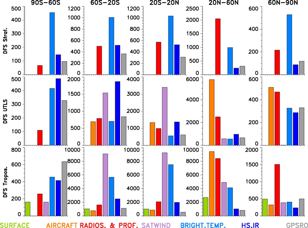
Degrees of Freedom for Signal (DFS) of the observing systems assimilated in Meteo-France global 4DVAR operational NWP system as of mid-2008. The results are binned by latitude and altitude bands (from bottom to top: troposphere, upper troposphere, lower stratosphere (UTLS), stratosphere). Observations from surface, aircraft, radiosonde, and wind profiler are typically referred to as “conventional”, SATWIND refers to Atmospheric Motion Vectors from satellite, BRIGHT. TEMP. refers to the brightness temperature radiances from HIRS, AMSU-A, AMSU–B, MHS, and SSM/I, HS.IR refers to hyperspectral infra-red brightness temperature radiances (AIRS and IASI), and GPSRO refers to GPS radio occultation.
Degrés de liberté du signal des différents systèmes d’observation assimilés dans le 4DVAR global opérationnel à Météo-France mi-2008. Les résultats sont groupés par bandes de latitudes et par bandes d’altitudes (de bas en haut : troposphère, troposphère supérieure et basse stratosphère, et stratosphère). Les observations depuis la surface, les avions, les radiosondes et les profileurs de vents sont données conventionnelles, ‘SATWIND’ désigne les vecteurs vents déduits depuis les satellites, ‘BRIGHT. TEMP.’ désigne les températures de brillance des instruments HIRS, AMSU-A, AMSU–B, MHS et SSM/I, ‘HS.IR’ désigne les températures de brillance des instruments infra-rouge hyperspectraux (AIRS et IASI), et ‘GPSRO’ désigne la radio-occultation GPS.

Operational NWP systems routinely upgrade their numerical models and assimilation models while adding on new sources of satellite observations. This results in improved forecast performance such as shown in Fig. 3 (left panel). It is however very difficult to separate in this improvement the contribution of model changes (e.g., resolution) and that of data assimilation.

Fig. 3
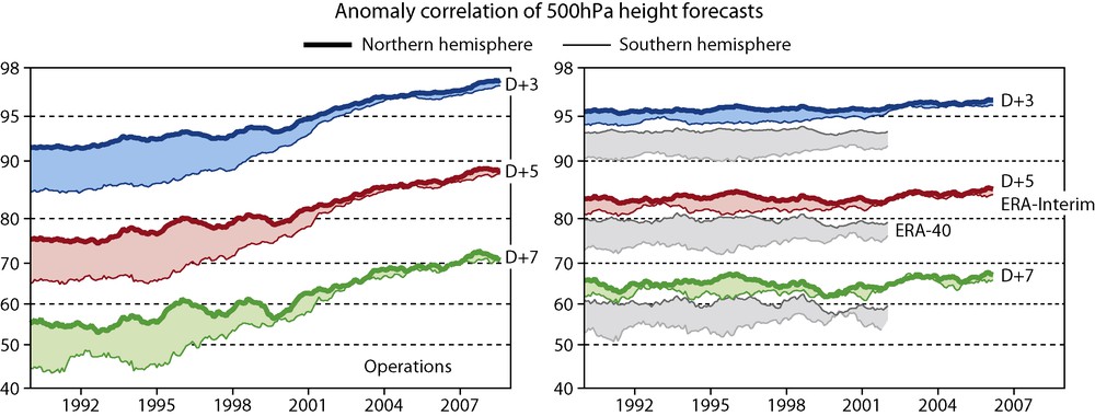
Timeseries of forecast error anomaly correlations (in percents) of 3-, 5-, and 7-day forecasts (labeled D+3, D+5, D+7, respectively), in the Northern Hemisphere (thick line) and the Southern Hemisphere (thin line) for ECMWF operations (left plot) and two generations of ECMWF reanalyses (right plot), ERA-40 and ERA-Interim. Each reanalysis uses a fixed forecast model throughout the whole reanalyzed time period. Figure courtesy of A. Simmons, ECMWF.
Séries temporelles des corrélations d’anomalies d’erreurs de prévisions (en pourcents) des prévisions à 3, 5 et 7 jours (marquées D+3, D+5, D+7, respectivement), dans l’Hémisphère Nord (traits épais) et l’Hémisphère Sud (traits fins), pour le système de prévision numérique du temps opérationnel au Centre européen de prévisions météorologiques à moyen terme (CEPMMT, figure de gauche) et deux générations de réanalyses (figure de droite), ERA-40 et ERA-Interim. Chaque réanalyse utilise un modèle de prévision à configuration figée pendant la période réanalysée. Figure fournie par A. Simmons, CEPMMT.

For that purpose, we extend our discussion to the European Reanalysis Projects, ERA-40 (Uppala et al., 2005) and ERA-Interim (Simmons et al., 2007). In each reanalysis, a fixed atmospheric model was used throughout the time period studied (1957–2002, and 1989–present, respectively). The only changes over time are (rare changes) in the sources of sea surface temperatures and the evolutions of the observing system over the whole time period. Assuming that the atmospheric predictability did not change significantly (though it has variations of its own), the time evolutions of forecast scores in reanalysis shown in Fig. 3 (right panel) may be interpreted to assess the impact of changes in the observing system. During the satellite-data rich era (post 1989), the improvement in forecast score in ERA-Interim are small (they appear to be more obvious after the introduction of AMSU-A, mid-1998). However, a similar figure (not shown here) but covering a longer time period, from conventional data only to modern times (1957–2002), shows that introducing VTPR data in 1972, and AMV and TOVS data in 1979, made clear marked impacts in ERA-40. Overall, with the NWP system used in ERA-40, the introduction of satellite data helped gain as much as three days of predictability in the useful forecast range (when scores fall below 60% correlation) as compared to the 1960s.

This quantitative improvement allowed by the introduction of new instruments is impressive but it should be emphasized that such improvement did not happen at once. It is only through long iterative loops of research, development, and trial (comparison with observations) that NWP systems have matured to the state where they can effectively assimilate all these data (with benefits for reanalysis, several decades after original data collection). The accomplishments of data assimilation have not only been to improve the quantitative forecasts through the provision of better conditions, but also to accompany the developments in NWP and bridge the gap between models and observations. This loop does not stop here as will be seen below.

7 Ongoing developments and future prospects

This section discusses the developments ongoing in data assimilation and the challenges ahead. On the methodology side, the first topic that is of immediate relevance to satellite data assimilation is the recent implementation in several systems of methods that correct for systematic differences (biases) between background and observations. Derber and Wu (Derber and Wu, 1998) applied early on concepts now known as variational bias correction. The idea is to solve for bias correction coefficients in the variational analysis, by introducing these coefficients as part of the state vector. The advantage of this method is that all the data contribute to determining the bias of a particular instrument. From an information point of view, this approach should be superior to any independent bias correction method alone, provided all the assumptions are satisfied. So far, this method has only been applied to the assimilation of passive infrared and microwave radiances, but other data could soon benefit from this approach.

A second topic of relevance is the development of methods to evaluate the impact of observations and the sensitivity of analyses to observations (Cardinali et al., 2004). This is especially important when it comes to understanding the sources of information feeding today's NWP systems. Another active topic of research is the automatic specification of observation and background errors (Desroziers et al., 2005). Another potential prospect is the refinement of observation operators to reproduce the slanted geometry of so-called nadir sounders. Out of all these topics, only the first one has reached the operational stage in various NWP systems.

There are also new approaches to data assimilation, such as weak-constraint 4DVAR discussed earlier. Another is the development of various filters to approximate the full Kalman filter, which is too expensive because it requires many model integrations in order to propagate the analysis error covariance matrix in time. Among these filters are the Extended Kalman Filtering (EKF), the Ensemble Kalman Filtering (EnKF), and the Ensemble Adjustment Kalman Filtering (EAKF) (see Ref. (Thomas et al., 2009) and references therein for a recent update). Also, Wang and Li (Wang and Li, 2009) recently proposed to extract the analysis information via a four-dimensional singular value decomposition.

On the satellite data side, one area of rapid current development is the assimilation of cloud and precipitation data. So far, the only cloud-affected data assimilated operationally are in the microwave range. The challenges before moving toward direct assimilation for all passive (microwave and infrared) data have to do with the large gap that separates today's NWP models from reality when it comes to the representation of cloud and precipitation microphysics. Reproducing the processes involved in the measurement process (scattering) requires complex modeling and (ideally) a good knowledge of the microphysical environment. As a result, the corresponding observation operators capable of carrying out such modeling are strongly non-linear. Another issue is the departure of the error distributions from Gaussian distributions. To the first order, this is related to the variability of water vapor, which cannot take on either negative values or values beyond saturation. Beyond that, the transitions between water phases represent discontinuous limits that translate themselves into non-continuous modeling processes. Overall, there are still several issues before the assimilation of such data becomes a research area of the past (Errico et al., 2007), but it is only through data assimilation and the iterative loop research-development-validation that this will become reality.

Furthermore, data assimilation offers a framework to extract value from past observations, even for decommissioned weather satellites whose data never got used in real-time. This framework is the reanalysis process (e.g., Uppala et al., 2005). It enables to make use of data (re-)processed with the latest science and algorithms. The apparently unchallenging exercises of data reprocessing and reanalysis enable one to learn new lessons from old data, by helping isolate and (ultimately) understand the sources of drift in satellite measurements. For example, Fig. 4 shows the HIRS bias corrections calculated by the now 20-year-long ERA-Interim reanalysis. The bias variations are usually found to be consistent with each other, with offsets between them. This could reflect differences between the satellites in the absolute calibration of the observations, or in the measurement modeling processes that are not fully understood. Note that HIRS NOAA-18, HIRS NOAA-19 and HIRS METOP-A stand out as compared to the other HIRS (see for example channel 2); they happen to be of a new generation (HIRS/4). Atmospheric reanalysis enables to improve our knowledge of the past weather for climatological or commercial purposes (e.g., insurance risk modeling). This is also a means to generate high-resolution datasets based on consolidated, quality-controlled observations and that can serve to improve today's seasonal forecast models. Ultimately, this will help better understand the discrepancies between what we think we know of the atmosphere (theory and modeling) and what observations actually tell us (reality and experiment).

Fig. 4
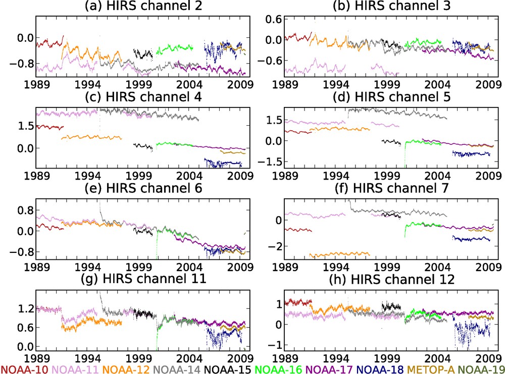
Variational bias corrections (radiance brightness temperature, in K) calculated by the ERA-Interim reanalysis for a selection of HIRS channels assimilated in that reanalysis. Refer to Fig. 1 for the correspondence between channels/satellites and vertical and spectral sounding regions. See http://www.ecmwf.int/research/era to access ERA-Interim products.
Corrections de biais variationnelles (températures de brillance, en K), calculées par la réanalyse ERA-Interim pour une sélection de canaux HIRS assimilés dans cette même réanalyse. Se référer à la Fig. 1 pour la correspondance entre canaux/satellites et les régions verticales et spectrales sondées. Consulter le site http://www.ecmwf.int/research/era pour accéder aux produits ERA-Interim.

Satellite data reprocessing may bring about new products especially useful in a reanalysis framework. One example is the reprocessing of the long record of Advanced Very High Resolution Radiometer (AVHRR, onboard the NOAA satellites) imagery. This would enable to derive AMVs over the Polar Regions in a fashion similar to MODIS AMVs. Another promising area of research is the extraction and assimilation of objects, such as vortex anomalies (Michel and Bouttier, 2006). An extension of this work to general imagery could enable using the large amounts of Earth image data (dating back to the 1960s), which have so far been largely ignored for quantitative atmospheric studies.

Overall, all the satellite observations of the atmosphere assimilated today originate from fundamental interactions of the electromagnetic waves with the atmosphere. Other Earth sciences already make use of a different form of fundamental interaction (gravity) with the Earth elements. For example, space geodesy measures gravity fields in order to retrieve information about the repartition of masses in the Earth system. The monitoring of precise satellite altimetry results from gravitational interaction of the gravity field with the satellite carrying the instrument. This enables to measure accurately the ocean height above a reference surface, but also to remotely sense groundwater storage. Both applications are relevant to meteorology since NWP requires boundary conditions over ocean and land. As the various Earth sciences are integrated into more sophisticated Earth system models, the importance of these different types of interactions (electromagnetic, gravitational) may bring complementary pieces of information.

8 Conclusions

Forty years after the first satellite measurements of the Earth's atmosphere, the prediction of the weather by numerical weather prediction has gained several days of improvement that can be attributed to the assimilation of satellite data. This measurable, objective impact must not hide that this improvement was gradual as numerical models and data assimilation schemes were upgraded in line with each other to benefit from these global data.

All the satellite observations of the atmosphere rely on the interaction of electromagnetic waves with matter. In data assimilation, so-called observation operators model these interaction mechanisms, reviewed in the present paper. Data assimilation forces the four-dimensional atmospheric representation to reproduce the observation data within bounds that are observation-error dependent.

As an ever-increasing number of observations of the atmosphere are collected, the challenges of data assimilation are now not only to keep up with this increase but also to expand towards so far rather unknown (poorly observed) quantities, such as aerosols and chemical species. Besides this forward-looking view, data assimilation also offers Earth scientists with a framework for integrating past data while benefiting from today's advanced modelling and computational facilities. Although comprehensive Earth-system models are still a long way in the future, atmospheric reanalyses already provide very complete environments for bringing together diverse data sources and understanding discrepancies between theory and reality. Briefly summarized, reanalyses enable to account for the aliasing problems inherent to the interpretation of climate trends from individual observing system data records affected by changes in observation practice (such as location, local time, and spectral sampling).

So far, data assimilation in meteorology (and now atmospheric studies in general) has greatly contributed by showing the way to the other Earth sciences. It may not be surprising if the years to come saw other areas of geophysical research, such as space weather, oceanography, and geodesy come up with new concepts in data assimilation, only waiting to be embraced by meteorology.

Bibliographie

[Baüer et al., 2006] P. Baüer; P. Lopez; A. Benedetti; D. Salmond; E. Moreau Implementation of 1D+4D-Var assimilation of precipitation-affected microwave radiances at ECMWF. I: 1D-Var, Q. J. R. Meteorol. Soc., Volume 132 (2006) no. 620, pp. 2277-2306 | DOI

[Benedetti et al., 2005] A. Benedetti; P. Lopez; P. Baüer; E. Moreau Experimental use of TRMM precipitation radar observations in 1D+4D-Var assimilation, Q.. J. R. Meteorol. Soc., Volume 131 (2005) no. 610, pp. 2473-2495 | DOI

[Bjerknes, 1904] V. Bjerknes Das Problem der Wettervorhersage, betrachtet vom Standpunkte der Mechanik und der Physik, Meteorologische Zeitschrift, Volume 21 (1904), pp. 1-7

[Cardinali et al., 2004] C. Cardinali; S. Pezzulli; E. Andersson Influence-matrix diagnostic of a data assimilation system, Q. J. R. Meteorol. Soc., Volume 130 (2004) no. 603, pp. 2767-2786 | DOI

[Charney, 1951] Charney, J. G. 1951. Dynamic forecasting by numerical process, Compendium of meteorology, Malone T.F. (Ed.), 470–482, Am. Meteorol. Soc., Boston.

[Chen et al., 2008] Y. Chen; F. Weng; Y. Han; Q. Liu Validation of the Community Radiative Transfer Model by using CloudSat data, J. Geophys. Res., Volume 113 (2008), p. D00A03 | DOI

[Daley, 1991] R. Daley Atmospheric Data Analysis, Cambridge U. Press, Cambridge, 1991 (457 p)

[Derber and Wu, 1998] J.C. Derber; W.-S. Wu The use of TOVS cloud-cleared radiances in the NCEP SSI analysis system, Mon. Wea. Rev., Volume 126 (1998) no. 8, pp. 2287-2299

[Desroziers et al., 2005] G. Desroziers; B. Chapnik; L. Berre; P. Poli Diagnosis of observation, background, and analysis error statistics in observation space, Q. J. R. Meteorol. Soc., Volume 131 (2005) no. 613, pp. 3385-3396 | DOI

[Errico et al., 2007] R.M. Errico; P. Baüer; J.-F. Mahfouf Issues regarding the assimilation of cloud and precipitation data, J. Atmosph. Sci, Volume 64 (2007) no. 11, pp. 3785-3798 | DOI

[Ghil et al., 1997] Data Assimilation in Meteorology and Oceanography: Theory and Practice (M. Ghil; K. Ide; A.F. Bennett; P. Courtier; M. Kimoto; N. Sato, eds.), Meteorol. Soc. Japan and U. Acad. Press, Tokyo, 1997 (496 p.)

[Grody et al., 2004] N.C. Grody; K.Y. Vinnikov; M.D. Goldberg; J.T. Sullivan; J.D. Tarpley Calibration of multisatellite observations for climatic studies: Microwave Sounding Unit (MSU), J. Geophys. Res., Volume 109 (2004), p. D24104 | DOI

[Healy et al., 2005] S.B. Healy; A.M. Jupp; C. Marquardt Forecast impact experiment with GPS radio occultation measurements, Geophys. Res. Lett., Volume 32 (2005), p. L03804 | DOI

[Kalman, 1960] R.E. Kalman A new approach to linear filtering and prediction problems, Trans. Am. Soc. Mechan. Eng., J. Basic Eng., Volume 82 (1960) no. 1, pp. 35-45

[Kalnay, 2003] E. Kalnay Atmospheric Modeling, Data Assimilation, and Predictability, Cambridge U. Press, Cambridge, 2003 (341 pp)

[Karbou et al., 2006] F. Karbou; E. Gérard; F. Rabier Microwave land emissivity and skin temperature for AMSU-A & -B assimilation over land, Q. J. R. Meteorol. Soc., Volume 132 (2006) no. 620, pp. 2333-2355 | DOI

[Kursinski et al., 1995] E.R. Kursinski; G.A. Hajj; K.R. Hardy; L.J. Romans; J.T. Schofield Observing tropospheric water vapor by radio occultation using the Global Positioning System, Geophys. Res. Lett., Volume 22 (1995) no. 17, pp. 2365-2368

[Lorenz, 1963] E.N. Lorenz Deterministic nonperiodic flow, J. Atmosph. Sci., Volume 20 (1963), pp. 130-141

[Marchand et al., 2009] R. Marchand; J. Haynes; G.G. Mace; T. Ackerman; G. Stephens A comparison of simulated cloud radar output from the multiscale modeling framework global climate model with CloudSat cloud radar observations, J. Geophys. Res., Volume 114 (2009), p. D00A20 | DOI

[Michel and Bouttier, 2006] Y. Michel; F. Bouttier Automated tracking of dry intrusions on satellite water vapour imagery and model output, Q. J. R. Meteorol. Soc., Volume 132 (2006) no. 620, pp. 2257-2276

[Parrish and Derber, 1992] D. Parrish; J.C. Derber The National Meteorological Center's spectral statistical interpolation analysis system, Mon. Wea. Rev., Volume 120 (1992) no. 8, pp. 1747-1763

[Pires et al., 1996] C. Pires; R. Vautard; O. Talagrand On extending the limits of variational assimilation in nonlinear chaotic systems, Tellus A, Volume 48 (1996), pp. 96-121

[Poli et al., 2007] P. Poli; P. Moll; F. Rabier; G. Desroziers; B. Chapnik; L. Berre; S.B. Healy; E. Andersson; F.-Z. El Guelai Forecast impact studies of zenith total delay data from European near real-time GPS stations in Météo France 4DVAR, J. Geophys. Res., Volume 112 (2007), p. D06114 | DOI

[Richardson, 1922] L.F. Richardson Weather Prediction by Numerical Process, Cambridge U. Press, Cambridge, 1922 (236 p)

[Sasaki, 1970] Y. Sasaki Some basic formalisms in numerical variational analysis, Mon. Wea. Rev., Volume 98 (1970) no. 12, pp. 875-883

[Saunders et al., 1999] R. Saunders; M. Matricardi; P. Brunel An improved fast radiative transfer model for the assimilation of satellite radiance observations, Q. J. R. Meteorol. Soc., Volume 125 (1999) no. 556, pp. 1407-1425

[Simmons et al., 2007] A. Simmons; S. Uppala; D. Dee; S. Kobayashi ERA-Interim: new ECMWF reanalysis products from 1989 onwards, ECMWF Newsl., Volume 110 (2007), pp. 25-35

[Smith, 1991] W.L. Smith Atmospheric soundings from satellites – false expectation or the key to improved weather prediction?, J. R. Meteorol. Soc., Volume 117 (1991) no. 498, pp. 267-297 | DOI

[Smith et al., 1972] W.L. Smith; H.M. Woolf; H.E. Fleming Retrieval of atmospheric temperature profiles from satellite measurements for dynamical forecasting, J. Appl. Meteorol., Volume 11 (1972) no. 1, pp. 113-122

[Stephens, 1994] G.L. Stephens Remote Sensing of the Lower Atmosphere: An Introduction, Oxford U. Press, 1994 (523 p)

[Tan et al., 2008] D.G.H. Tan et al. The ADM-Aeolus wind retrieval algorithms, Tellus A, Volume 60 (2008) no. 2, pp. 191-205 | DOI

[Thomas et al., 2009] S.J. Thomas; J.P. Hacker; J.L. Anderson A robust formulation of the ensemble Kalman filter, Q. J. R. Meteorol. Soc., Volume 135 (2009) no. 639, pp. 507-521 | DOI

[Trémolet, 2007] Y. Trémolet Model-error estimation in 4D-Var, Q. J. R. Meteorol. Soc., Volume 133 (2007) no. 626, pp. 1267-1280 | DOI

[Uppala et al., 2005] S.M. Uppala et al. The ERA-40 re-analysis, Q. J. R. Meteorol. Soc., Volume 131 (2005) no. 612, pp. 2961-3012 | DOI

[Wang and Li, 2009] J. Wang; J. Li A four-dimensional scheme based on singular value decomposition (4DSVD) for chaotic-attractor-theory-oriented data assimilation, J. Geophys. Res., Volume 114 (2009), p. D02114 | DOI

Commentaires - Politique

Ces articles pourraient vous intéresser

Observing the atmospheric wind from space

Alain Dabas

C. R. Géos (2010)

Observation of the thermal structure and dynamics of the stratosphere and the mesosphere from space

Alain Hauchecorne; Philippe Keckhut; Chantal Claud; ...

C. R. Géos (2010)

Precipitation retrieval from space: An overview

Catherine Prigent

C. R. Géos (2010)