

1 Introduction
Together with pressure, temperature and humidity, wind is one the few variables that characterize the thermodynamic state of the atmosphere. Its prediction has always received much attention, as strong winds can cause heavy damage and deaths (for instance, the International Meteorological Organization – the ancestor of the current World Meteorological Organization – was created in the second half of the 19th century after a wind storm destroyed several French and British warships besieging Sebastopol during the Crimean war. A study conducted by the French astronomer Le Verrier showed that the storm had swept across Europe before touching Crimea and could have been predicted by a proper observation network). However, compared to temperature or humidity, wind is poorly observed. This is particularly true for the observations from space, which are currently limited to the measurement of the movement of clouds or distinctive water vapor features between successive geostationary satellite images, or sea surface winds by radar scatterometry.
There are probably two major reasons for this. The first relates to the physics of the atmosphere. At the mid and high latitudes that are of most interest to the European countries or the United States of America, the wind is governed by the mass field through the well-known geostrophic equilibrium:
The second reason is technical: observing the wind from space proved much more difficult than e.g. temperature, as the latter can be sensed with passive sensors, while the former requires active ones (with the exception of the winds derived from satellite images as discussed below).
Today, thanks to the progress made in satellite observation and numerical weather prediction, the mass field in the atmosphere is known with a good precision. Meteorological analyses of the temperature for instance have a precision of the order of 1 or 2 K, sometimes even better. The geostrophic wind is thus well characterized. In spite of this, the interest for direct wind observations has not diminished because current weather prediction models are now global and are resolving fine space and time scales where the geostrophic equilibrium is not operating anymore. The domain of applicability of the geostrophic equilibrium is limited to the atmospheric phenomena that have a typical size L longer than the Rossby radius of deformation R (Holton, 2004).
The growing interest for small scales in the atmosphere (phenomena with a size smaller than R) or the Tropics has led the World Meteorological Organization to set a high priority on the improvement of wind observation capabilities (WMO, 2003). In answer to this priority, the European Space Agency started a program in 2005 called ADM-Aeolus with the aim of launching the first wind sensor ever operated from space. Based on lidar technology, this mission will measure winds over the entire globe and throughout the whole depth of the atmosphere, delivering its data to the weather prediction centers in less than 3 hours. Built on the expertise acquired in the 1980s and 1990s by various research teams around the world, this technically challenging program is well under way, with the launch planned for late 2011.
2 What observations are currently available?
Weather prediction relies on the large number of observations carried out over the entire globe and made available to meteorological centers via the Global Telecommunication System (GTS). The observations are used to determine the state of the atmosphere at a particular time, the so-called analysis. The analysis serves as the initial state of numerical weather predictions. Starting from this state, the differential equations that govern the dynamics of the atmosphere are integrated by the numerical model into a prediction. As the number of observations is much less than the total number of model unknowns, the computation of the initial state requires some additional information that is in practice provided by the previous weather forecast – the so-called “first guess”. The operation that mixes the first guess and observation is called assimilation. This data-fusion process computes the differences between the first-guess and the observations, and modifies the first guess so that both match. The modification of the first-guess must be done very carefully, it must not introduce unrealistic features that would destabilize the forecast or violate the fundamental laws of the atmospheric physics (for instance, a large-scale modification of the wind field requires that a large scale modification of the pressure field is also brought otherwise the geostrophic equilibrium will not be verified anymore). At Météo-France, the global model ARPEGE is run 4 times a day at 00 UTC, 06 UTC, 12 UTC and 18 UTC. Each run contains an assimilation. The first step of the assimilation consists of a screening procedure that aims at discarding the observations that are too far off the first-guess and thus appear to be gross errors. For many information types, the number of observations that are tagged as gross errors can be very large and represent more than 90% of the total number of observations.
The nature and volume of wind observations available for weather forecast is detailed in Table 1. They are grouped in three major classes (column 1) depending on whether they are obtained from a satellite, or are surface measurements acquired by surface based sensors (Surface), or are altitude winds.
Observations de vent disponibles à la prévision météorologique. La colonne 1 indique si l’observation vient d’un satellite, d’une station de surface à terre ou en mer, ou de tout autre type de capteur non-satellitaire capable de fournir des observations en altitude. Dans la colonne 2, on retrouve le nom des messages qui contiennent l’information. Pour les données spatiales, il y a deux messages possibles, les SATOB qui contiennent des mesures de vent obtenues par le suivi de motifs distinctifs (nuages par exemple) dans les images spatiales. Ils sont pour la plupart issus des satellites géostationnaires, mais certains proviennent également des satellites en orbite polaire. Les diffusomètres déduisent le vent, à la surface de la mer, de l’intensité de la diffusion par cette dernière des micro-ondes qu’ils émettent. En surface, les mesures de vent peuvent provenir de capteurs in situ dédiés localisés à terre (SYNOP) ou en mer sur des bateaux (SHIP) ou des bouées (BUOY). Pour ce qui concerne l’altitude, les mesures de vent sont réalisées par radiosondage (TEMP), suivi de ballons (PILOT), ou par des radars profileurs. Une dernière source d’information est constituée par les avions de ligne spécialement équipés pour la mesure météorologique. Les chiffres indiqués dans la troisième colonne sont les nombres journaliers moyens d’observations livrées à temps à Météo-France en novembre 2008. Il faut noter que le nombre de données effectivement assimilées par le modèle est inférieur, à cause de l’opération d’écrémage qui précède l’assimilation elle-même.
| Type | Description | N/day | Comment | |
| Satellite | SATOB | Wind vectors measured from the movements of clouds or water vapor features observed from satellite images | 1000 hPa – 700 hPa: 700,000 700 hPa – 400 hPa : 100,000 400 hPa – 150 hPa: 600 000 |
|
| Scatterometer | Surface winds measured from the scattering of micro waves by the sea surface (Quickscat, ERS2, METOP A) | 700,000 | Sea surface level information ERS and METOP : 5.3 GHz Quickscat: 13.4 GHz | |
| Surface | SYNOP | Surface stations. Winds at 10 meters above the surface | 100,000 | Surface winds. Irregular density (strong density over populated regions, light density otherwise) |
| SHIP | Sea surface winds measured from a ship | |||
| BUOY | Sea surface winds measured from a buoy | 3500 | ||
| Altitude | TEMP | Radio sounding | 1500 | Great majority from fixed synoptic stations at land. A few from instrumented, commercial ships. Irregular geographical distribution. |
| PILOT - Profiler | Ballon tracking or radar profilers | 4000 | From fixed station at land. Irregular geographical distribution | |
| Aircrafts | Measurements by instrumented aircrafts | 200,000 |
Surface winds are measured by in situ sensors (anemometers) based either on land or at sea on ships or buoys. The geographical distribution of these types of observations is highly irregular (Fig. 1). Most of them are obtained in highly populated regions of the globe, and large, desert areas (open sea, Sahara, polar regions, tropical rain forest…) are almost completely empty. Although the technology involved is rather simple, their total number is relatively small (about 100 000/day) because telecommunications are necessary to deliver the measurements in a time period short enough (in less than a few hours in practice) so that they can be assimilated. This requirement restricts the number of possible sites to a rather small number of stations equipped with wired or wireless telecommunication systems (buoys, for instance, transmit their data via expensive satellite communication links). In addition, many of these observations do not pass the screening phase of the assimilation. This does not mean that they are not of good quality – indeed, many of them are of good quality – but they suffer from an inherent drawback common to all surface measurements: they are influenced by local effects – topography for instance – that the forecasting models are not able to represent correctly. Thus, they bring information that the model cannot use properly and they may even destabilize the forecasting process.

Position of the SYNOP and SHIP messages that were available at Météo-France on the 3rd of February 2009 when the numerical weather prediction run of 00 UTC was started. The density is high in rich, populated areas, but much lighter over the oceans and the deserts, leaving large gaps in the coverage.
Localisation des messages SYNOP et SHIP disponibles à Météo-France le 3 février 2009 pour le cycle de prévision numérique de 00:00 UTC. La densité est élevée dans les régions riches et fortement peuplées, mais en revanche légère sur les océans ou dans les déserts. Des régions entières sont très peu observées.
Altitude wind observations are more numerous as their number exceeds 200,000. However, this figure must be considered with care as 97.5% of the observations are provided by commercial aircrafts specifically equipped for weather observation. This information is of great value for aviation as it characterizes the weather conditions prevailing on major flight routes or in the approach areas of airports (for instance, it enables precise predictions of gas consumption or time of arrival), but for weather prediction, these observations suffer from a major limitation: most of them are along a limited number of flight routes (Fig. 2) and characterize the wind at the typical flight altitude of ∼10 km.

Position of aircraft messages that were available at Météo-France on the 3rd of February 2009 when the numerical weather prediction run of 00 UTC was started. The geographical distribution is highly irregular, the observations are concentrated along the main flight routes, at an altitude of about 10 km (cruising altitude of commercial jets).
Position des mesures contenues dans les messages météorologiques fournis par les avions de ligne, disponibles à Météo-France pour la prévision du réseau de 00:00 UTC le 3 février 2009. La répartition géographique est très inégale. Les mesures sont essentiellement concentrées le long des grands couloirs aériens, à 10 km d’altitude (altitude de croisière des avions).
TEMP messages contain the observations made by radiosounding systems. A radio sonde is a small and light device that combines several probes, usually for temperature, humidity and pressure. The sonde is attached to a balloon inflated with nitrogen. As it is lighter than the air, the balloon goes up in the atmosphere with the sonde underneath. Along the ascent, the sonde transmits the temperature, pressure and humidity measurements by a radio frequency link. The position of the balloon relative to receiving station at the surface is determined by a tracking system which nowadays is generally a differential GPS (Global Positioning System). The wind is derived from this information. Today, radio-sondes are considered the reference for altitude winds because they are accurate and reliable. In spite of this, their number is very limited around the Earth (Fig. 3) because they are expensive (the cost of the radio-sonde is of the order of 100 €, and a radiosounding requires the work of an operator for more than an hour). Most of the radio sounding stations are in rich countries, and operated only 2 or 4 times a day. In continental France for instance, seven radio sounding stations launch balloons two times every day at 00 and 12 UTC.
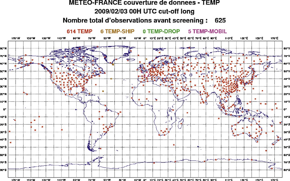
Same as Fig. 1 for radio sondes.
Idem Fig. 1, mais pour les radiosondages.
Like TEMP, PILOT gives wind information obtained by tracking a balloon, but this time the balloon has no sonde attached to it. The wind is derived from the time derivative of its position determined by optical or radar tracking.
3 Techniques available from space
Two different sources of information on wind are available from space. One is called SATOB. SATOB winds are derived from satellite images. Distinctive features – clouds or water-vapor structures – are tracked across successive images of the same scene in either the visible, the infra-red or the water vapor channel. Their apparent movement is then converted into a wind information. The altitude of the information is computed from the infrared brightness temperature of the cloud top (or water vapor structure). The images come mostly from geostationary satellites (Meteosat in Europe, GOES in the USA…) that offer the advantage of always looking at the same point of the Earth and a fast repetition rate (one image every 15 minutes with Meteosat Second Generation). For several years now, the concept has also been applied to images from polar orbiting satellites – in particular TERRA and AQUA from the National Aeronautics and Space Agency of the United States of America.
SATOB provides a large set of wind data – about 1,500,000 pieces of information every day – with a good geographical coverage (with the exception of the high latitudes that are not seen by the geostationary satellites – Fig. 4) and an altitude range from the near-surface to altitudes as high as 100 hPa (or ∼15 km). However, they suffer from major limitations. SATOB does not provide vertical profiles of wind but only one measurement at the cloud top altitude for a given latitude and longitude. It is thus not possible to document possible wind shears along the vertical. Wind measurements are restricted to cloud regions – no information is available in cloud-free regions – and the number of measurements is reduced during night time when no visible images are available anymore.
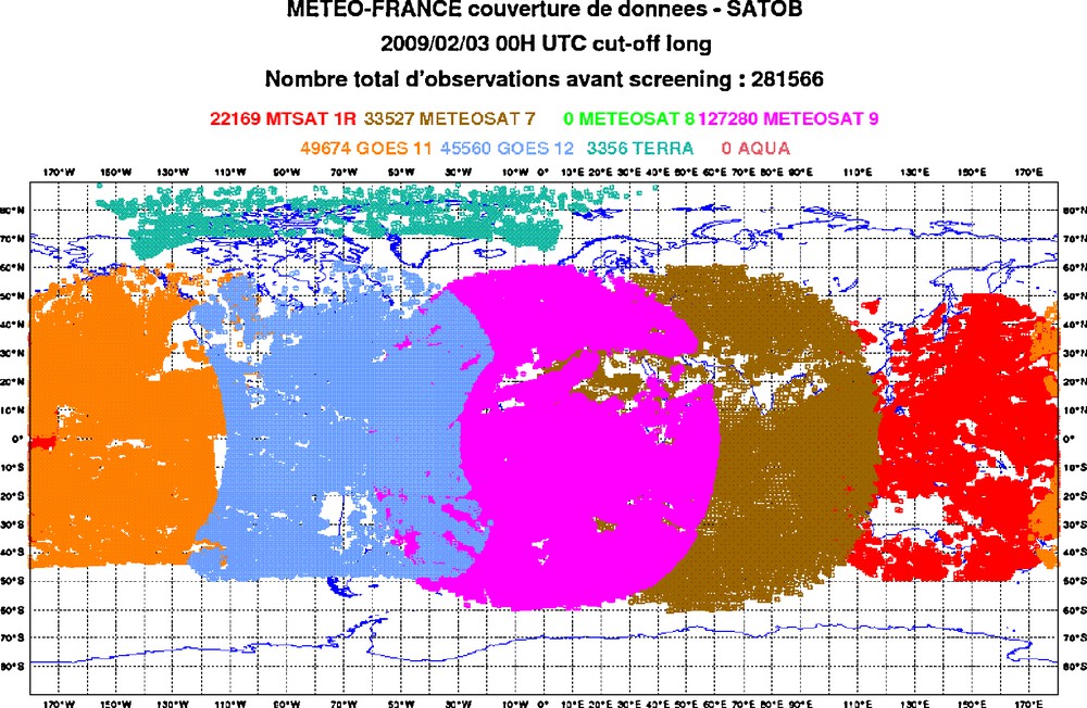
Same as Fig. 1 for SATOB.
Idem Fig. 1 pour les SATOB.
A second source of information from space is the various scatterometers that are permanently flying around the Earth in low-level, polar orbits. Scatterometers are active remote sensors operating in the microwave frequency domains (frequencies between 5 and 15 GHz). They measure images of the scattering cross-section of the surface (that is, the ability of the surface to reflect the radio wave back to space). Over the ocean, the radar cross-section varies as a function of the wind force and direction relative to the azimuth of the radar beam. By combining several beam directions, the wind force and direction can be estimated.
Fig. 5 shows the European polar-orbiting meteorological satellite METOP-A with the Advanced Scatterometer ASCAT on board. The three double antennas of ASCAT are visible below the spacecraft. They measure the sea-surface cross-section in two swaths centered at an inclination of 36 degrees to the left and the right of the satellite track. Each swath is 550 km wide, the horizontal resolution of sea-surface wind measurements is 50 km.
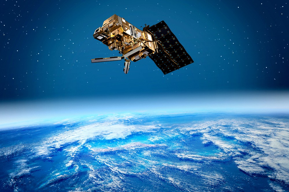
Artist's view of the European, polar-orbiting satellite METOP-A. The three (double) antennas of the Advanced Scatterometer (ASCAT) can be seen below the spacecraft. They provide measurements of the sea-surface scattering cross-sections with three different azimuth angles in two parallel swaths. The swaths are 550 km wide, they are centered at an inclination of 36 degrees to the left and right of the satellite track. The horizontal resolution is 50 km.
Vue d’artiste du satellite européen en orbite polaire METOP-A. On peut voir les trois antennes doubles du diffusomètre ASCAT (Advanced Scatterometer) sous le véhicule spatial. Elles fournissent des mesures de la section efficace de diffusion de la surface de la mer selon trois angles azimutaux différents à l’intérieur de deux fauchées parallèles de 550 km de large et situées à 36° de part et d’autre de la trace. La résolution horizontale est de 50 km.
Scatterometers provide a wind information in regions – the oceans – that are otherwise poorly documented by other wind observation systems. They have the advantage that they can make measurements in all types of weather conditions. For instance, they are able to measure winds below cyclones and thus provide observations of great value for the forecasting of such dangerous weather hazards. However, the observations are restricted to the surface, they give no information at all on the vertical structure of the atmospheric dynamics.
4 The spaceborne Doppler lidar ADM-AEOLUS
In the late 1990s, the European Space Agency (ESA) decided and started a mission for a space-based Doppler lidar. The decision came after several studies that refined the scientific requirements and showed the system was technically challenging, but feasible, and a selection process that culminated in 1999 when the program entered the phase B of its development cycle. The program is called ADM-Aeolus, ADM standing for Atmospheric Dynamics Mission. It is planned to be launched during the second semester of 2011.
ADM-Aeolus is the second mission of the Earth-Explorers program of ESA (information on the program can be found online at http://www.esa.int/esaLP/LPearthexp.html, or in (ESA, 1998). Its aim is to measure winds at the global scale throughout the entire depth of the meteorological atmosphere (Andersson et al., 2008; Stoffelen et al., 2005). The mission is based on a Doppler lidar. The wind is measured by estimating the frequency Doppler shift Δν between a laser pulse emitted by the instrument and the light that the atmosphere scatters back to the satellite. According to Doppler's equation, the Doppler shift is proportional to the component vr of the wind along the laser beam (the so-called radial velocity):
Here, λ is the laser wavelength (λ = 355 nm for ADM).
The measuring geometry of ADM is depicted in Fig. 6. ADM will fly along a polar orbit at about 400 km above the Earth-surface. The laser beam is always directed perpendicular to the flight track with a nadir angle of 35 degrees (optimal compromise between the sensitivity to the horizontal wind that increases with the nadir angle and attenuation of the laser beam with the distance along the line-of-sight that is weaker when the lidar is pointing closer to the nadir). The perpendicular line-of-sight offers the advantage that the satellite speed has no impact on the frequency Doppler shift (its component on the laser beam direction is null). However, it also follows that ADM will measure a single component of the wind, the east–west component – and will be almost insensitive to the north–south component.

Measurement geometry of ADM-Aeolus. The lidar directs the laser beam in a fixed direction perpendicular to the flight track with a nadir angle of 35 degrees. The light returned by the atmosphere is accumulated during 7 seconds before it is analyzed, resulting in a horizontal resolution of 50 km. The laser is switched off between two 7 second burst, so there is a gap of 150 km between two wind profile measurements resulting in a horizontal sampling interval of 200 km. The light captured by the telescope of the lidar is analyzed by two different detection channels, the Rayleigh channel for the molecular part, and the Mie channel for the aerosol one. Both have independent vertical gates. In the aerosol channel, the gating focuses on the low levels of the atmosphere with an enhanced vertical resolution, while the molecular channel extends the vertical coverage to the lower stratosphere at the expense of a degraded resolution. Masquer
Measurement geometry of ADM-Aeolus. The lidar directs the laser beam in a fixed direction perpendicular to the flight track with a nadir angle of 35 degrees. The light returned by the atmosphere is accumulated during 7 seconds before it is analyzed, ... Lire la suite
Géométrie de mesure d’ADM-Aeolus. Le lidar dirige le faisceau de sondage perpendiculairement à l’orbite du satellite avec un angle de 35° par rapport à la verticale. La lumière renvoyée par l’atmosphère est intégrée pendant 7 secondes avant d’être analysée. Pendant ce temps, le satellite ayant parcouru 50 km, il en résulte une résolution horizontale de la mesure de 50 km. Après ces 7 secondes, le laser est éteint pendant 21 secondes pendant lesquelles le satellite parcourt 150 km, d’où un pas d’échantillonnage spatial de 200 km le long de la trace. La lumière captée par le télescope est analysée sur deux voies de détection, l’une – la voie Rayleigh – dédiée à la rétrodiffusion moléculaire, l’autre – la voie Mie – à la rétrodiffusion particulaire. L’échantillonnage vertical est indépendant sur les deux voies. Sur la voie Mie, les portes de mesures cherchent à documenter le vent avec une résolution verticale fine dans les basses couches de l’atmosphère, tandis que sur la voie Rayleigh, l’accent est mis sur la haute troposphère et la basse stratosphère. La résolution verticale y est plus grossière. Masquer
Géométrie de mesure d’ADM-Aeolus. Le lidar dirige le faisceau de sondage perpendiculairement à l’orbite du satellite avec un angle de 35° par rapport à la verticale. La lumière renvoyée par l’atmosphère est intégrée pendant 7 secondes avant d’être analysée. Pendant ce ... Lire la suite
The narrow laser beam (the spot has a diameter of ∼200 meters at the surface) hits the Earth at a distance of ∼300 km to the side of the flight track. Laser pulse returns are accumulated during 7 seconds so the wind profiles have a horizontal resolution of 50 km. The laser is switched off between two 7-second burst, leaving a gap in the horizontal sampling of ∼150 km between two profiles. The observational requirements set at the beginning of the mission design are listed in Table 2. The vertical resolution of the actual lidar will vary from about 250 m in the planetary boundary layer (better than the 500 m of the observational requirements) to 1 km in the free troposphere and 2 km in the stratosphere, for an accuracy of 2 ms−1 to 5 ms−1.
Cahier des charges d’ADM-AEOLUS en termes de capacité d’observation (Andersson et al., 2008).
| Observational Requirements | |||
| PBL | Troposphere | Stratosphere | |
| Vertical Domain (km) | 0–2 | 2–16 | 16–30 |
| Vertical Resolution (km) | 0.5 | 1 | 2.5 |
| Horizontal Domain | Global | ||
| Number of profiles (hour−1) | 100 | ||
| Profile separation (km) | 200 | ||
| Temporal sampling (hour) | 12 | ||
| Accuracy (component) (ms−1) | 2 | 2–3 | 3–5 |
| Dynamic range (ms−1) | ± 150 | ||
| Horizontal Integration (km) | 50 | ||
| Error correlation | 0.01 | ||
| Probability of Gross Error (%) | 5 | ||
| Timeliness (hour) | 3 | ||
| Length of observational Data Set (year) | 3 |
ADM implements two channels of detection, one dedicated to the analysis of the frequency shift of the light backscattered by the molecules, the other one for aerosol returns. The need for two detection channels arises from the fact that the spectrum of the molecular backscatter is broadband (proportional to the square root of the temperature, the width of the molecular spectrum is several Gigahertz) while the aerosol return is narrow-band (a few hundreds of megahertz in width). The frequency shift of the molecular return is determined by passing the light through two Fabry-Perot filters centered on either side of the emitted frequency (Fig. 7). This is the so-called double-edge technique described in Garnier and Chanin, 1992. When the Doppler shift is zero, the number of photons NA and NB counted at the output of the two filters are equal. When the Doppler shift moves the molecular spectrum to the right (left), NA (NB) increases while NB (NA) decreases. The Doppler shift is obtained by inverting the relationship between the instrument response defined as R = (NA-NB)/(NA + NB) and the Doppler shift. The inversion is done by applying calibration curves. Details can be found in Dabas et al., 2008.
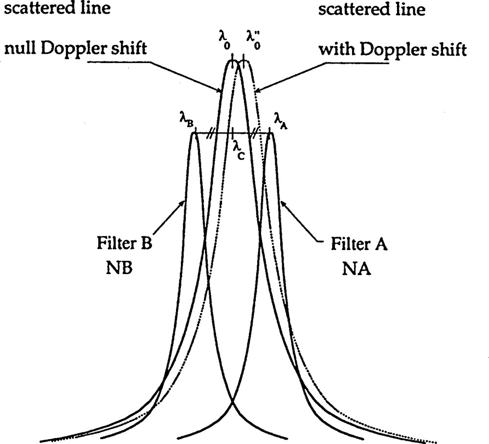
Diagram showing how the molecular channel of ADM Aeolus works (Garnier and Chanin, 1992). The light received by the lidar is passed through two filters A and B centered on either side of the molecular spectrum. When the Doppler shift is zero, the number of photons NA and NB counted at the output of the two filters are equal. When the Doppler shift moves the molecular spectrum to the right (left), NA (NB) increases while NB (NA) decreases. The Doppler shift is obtained by inverting the relationship between the instrument response defined as R = (NA − NB)/(NA + NB) and the Doppler shift. Masquer
Diagram showing how the molecular channel of ADM Aeolus works (Garnier and Chanin, 1992). The light received by the lidar is passed through two filters A and B centered on either side of the molecular spectrum. When the Doppler ... Lire la suite
Schéma montrant comment la voie moléculaire parvient à mesurer le vent (Garnier and Chanin, 1992). La lumière captée par le lidar passe à travers deux filtres optiques A et B centrés de part et d’autre du spectre moléculaire. En cas de décalage Doppler nulle, les nombres NA et NB de photons transmis par les filtres A et B et effectivement détectés sont égaux. Lorsque, par effet Doppler, le spectre moléculaire est décalé vers la droite (gauche), NA (NB) augmente alors que NB (NA) diminue. Le décalage Doppler peut alors être estimé par inversion de la réponse instrumentale définie par la relation R = (NA − NB)/(NA + NB). Masquer
Schéma montrant comment la voie moléculaire parvient à mesurer le vent (Garnier and Chanin, 1992). La lumière captée par le lidar passe à travers deux filtres optiques A et B centrés de part et d’autre du spectre moléculaire. En ... Lire la suite
For the narrow-band aerosol return, the Doppler shift analysis is based on a fringe-imaging technique: the atmospheric return received by the lidar is passed through a Fizeau interferometer. A fringe is formed between the two plates of the interferometer at a position proportional to the frequency Doppler shift. The fringe is imaged on a CCD by a proper optical arrangement. The position of the image on the CCD is computed from the number of photons counted by the CCD pixels (in ADM, the CCD is a square of 20 lines by 20 columns of pixels), it gives the position of the fringe in the Fizeau which in turn provides the Doppler shift estimation.
ADM-Aeolus will measure vertical profiles of one wind component, giving information on the possible wind shears. A major limitation of the system is that it cannot penetrate clouds (at the exception of the thin ones). It follows that there will be no wind information inside and below thick and extended cloud covers. When the cloud cover is broken, a limited number of narrow laser beams should be able to go through and sound the air masses below. Provided there are enough of them, it should be possible to measure their wind profiles. At last, optically thin clouds like cirrus are causing no problems. Not only are they only weakly attenuating the laser beam, but they also provide strong Mie returns that the lidar can use in order to measure accurate winds at the cloud altitude. Overall, the number of individual wind measurements made every day should be of the order of 50,000 to 100,000 on average (depending on the cloud cover). They will be delivered to the meteorological centers in less than 3 hours so they can be assimilated by most numerical weather prediction systems ((see Tan et al., 2008) for details on the processing and assimilation of ADM wind data).
For the weather centers that wish to assimilate ADM data, a portable version of the level-2 processors of the mission has been developed for deriving all the information needed for the assimilation of the wind data, and are available to any center that requests for it.
Processors and data will also be made available to the research community. Data will include wind measurements but also optical products like vertical profiles of the aerosol backscatter and extinction coefficients of the atmosphere. These latter products are obtained from the intensities of the molecular and aerosols returns through a complex processing scheme described in (Flamant et al., 2008). They will complement the large base of atmospheric data products collected by the CALIPSO mission (see http://www-calipso.larc.nasa.gov/ for details).
5 Conclusion
Although wind is a basic variable of the atmospheric state, it is rather poorly observed by existing observation systems. Ground-based systems deliver surface winds in mostly rich, populated regions of the Earth, leaving large gaps in the coverage above the oceans or deserts. In the upper levels, the major sources of data outside space are the reliable, but costly radio sondes and equipped commercial aircrafts. Both suffer the same type of limitations as ground-based systems, their geographical coverage is highly irregular, limited to the flight routes for the latter. First observations of wind from space were made by tracking clouds in visible satellite images. Called SATOB, they were extended to the infrared domain and the tracking of water vapour structures; they are today a major source of information for the wind. Their geographical coverage is nearly uniform (except for the high latitudes unseen by geostationary satellites), but the vertical structure of the atmospheric dynamics remains unresolved as SATOB relies on 2D images. For a given atmospheric column, there is a maximum of two wind measurements available (two wind components). The scatterometers complement the observation system by providing sea-surface winds. Their observations have proven to be very useful – for hurricane forecast for instance – they cover regions, the oceans, that are otherwise poorly sampled by ground-based systems.
Today the major gap in the wind observation system is the altitude, cloud free regions of the atmosphere. The space-based wind lidar ADM-Aeolus of the European space agency should fill when it is launched in 2011, as it is primarily targeted to the cloud free regions of the atmosphere and provides whole vertical profiles of one wind information.
Vous devez vous connecter pour continuer.
S'authentifier