

1 Introduction
Multiphase flow is widely encountered in the fields of hydrology and environmental engineering sciences in the context of soil and groundwater pollutions of non-aqueous phase liquids (NAPL), such as chlorinated solvents; they constitute a large and serious environmental problem (Cohen and Mercer, 1993). In addition, in soil and groundwaters, they are subject to natural attenuation. Identification of pollution sources is difficult due to the fact that organic pollutants can rapidly migrate down to the bottom of the aquifer and/or along paths different from the water (Bano et al., 2009; Benremita and Schäfer, 2003; Bohy et al., 2004, 2006; Dridi et al., 2009). Among the different attenuation processes involved, such as dispersion, adsorption, volatilisation, chemical and biological destruction, biodegradation is often considered most important (Nex et al., 2006; Sinke and Le Hecho, 1999). Taking into account all of these mechanisms to quantify and characterise groundwater pollution by NAPLs, multicomponent transport equations require a fast and accurate resolution of three-phase flow primary and secondary variables.
Two different strategies are currently used to model multiphase flow in porous media (Helmig, 1997). Using the first approach, in the case of a NAPL migrating in an unsaturated zone, the water-oil-gas three-phase system can be modelled by three pressure equations obtained by introducing the Darcy velocities of each fluid phase into the individual mass balance equations. This system of pressure equations can be transformed into a pressure-saturation form by using relationships between the wetting phase saturation and the capillary pressure, which is defined as the pressure difference across the interface between a non-wetting and a wetting phase. The pressure of the second and third fluid phases can then be removed by expressing this pressure in terms of the saturation and pressure of the other phase. This latter approach is useful when phase disappearance occurs and saturation becomes zero. The system of partial differential equations describing a three-phase flow is highly non-linear due to the nature of the relative permeability and capillary pressure functions needed to close the system.
Alternative forms of these governing flow equations have been investigated to develop better computational algorithms. This has led to the fractional flow approach, which originates from the petroleum industry. In this approach, the total fluid flow describes the individual phases as a fraction of the total flow (Binning and Celia, 1999). Through the fractional flow formulation, the immiscible displacement of oil, gas and water can usually be expressed in terms of three coupled equations, namely a mean pressure equation (Nayagum et al., 2001, 2004) or global pressure equation (Antoncev and Monahov, 1978; Chavent and Jaffré, 1986) and two saturation equations.
In this article, a fractional three-phase flow formulation is chosen using a global pressure approach. Numerical simulation of three-phase compressible flow in a porous medium usually requires the knowledge of the corresponding three-phase data. Experimental values for relative three-phase permeabilities and capillary pressures are usually known only for three two-phase sides of a water-oil-gas triangular diagram T. Three-phase relative permeabilities are generally derived from these sets of two-phase data by interpolation formulas (Baker, 1988; Stone, 1970, 1973). The compressible flow equations reformulated in terms of the global pressure and saturations of the gas and water phases are derived under the assumption that the three-phase data satisfy the total differential (TD) condition (Amaziane and Jurak, 2008; Chavent and Jaffré, 1986). This condition allows the two gradients of two-phase capillary pressure to be rewritten as a single gradient of a mathematical function called the global capillary function.
Comparisons with classical approaches such as pressure-pressure or pressure-saturation formulations have shown the computational efficiency of the global pressure-saturation formulation, as it reduces the coupling between pressure and saturation equations (Chen, 2005; Chen and Ewing, 1997). The aim of this article is to compare two different parameterisation approaches used to assess the reformulated three-phase data needed to simulate three-phase flow.
To assess the three-phase data, a step-by-step algorithm based on the approximated global pressure formulation was originally proposed by Chavent and Salzano (1985), and Chavent and Jaffré (1986) for compressible three-phase flow. It is derived under the TD condition so that each of the three-phase volume factors are evaluated at the global pressure level instead of their own phase pressure. The two corresponding degrees of freedom of this original interpolation are fractional flow functions fj for each fluid phase j and the global mobility d. Resulting TD three-phase data are ultimately determined with the resolution of two constrained optimization problems.
Recently, a new class of TD-interpolations algorithm was introduced by Chavent (2009), Chavent et al. (2008), and di Chiara Roupert et al. (2010), which allows the use of an exact global pressure formulation. The phase volume factors are evaluated at their own phase pressure. The two degrees of freedom of this new class of TD interpolation include the global capillary function
- • monotonicity, regularity and bound constraints of the resulting three-phase data;
- • the TD condition introduced in the mathematical model to simplify the pressure equation in the three-phase flow model.
In this article, we analyse the implementation of both approaches and assess the numerical results obtained in the case of two-phase data for a typical homogeneous porous medium. In the first section, the exact global pressure approach is employed using the conventions introduced by Chavent (2009) and Chavent et al. (2008). This leads to a simplified water and gas saturation equation and an expression of the pressure equation under Darcy's law. Then, we briefly discuss the implementation of both interpolation approaches to obtain three-phase TD data, which coincide with the given two-phase data set on the boundaries of the ternary diagram. Finally, in the fourth section we show numerical results, including the TD-interpolated water fractional flows, global mobilities and the global capillary function obtained by both approaches for an incompressible test case. Finally, we highlight practical aspects concerning the use of these two approaches in the context of a flow simulator.
2 Governing equations for three-phase flow in porous media
Let us recall the equations associated with the reformulated three-phase flow under the TD condition. The following notations are used for three fluid phases: j = 1 indicates water, j = 2 indicates oil, j = 3 and indicates gas.
2.1 Global pressure equation
We introduce the volume factor Bj evaluated at a pressure level p:
| (1) |
| (2) |
| (3) |
| (4) |
| (5) |
| (6) |
| (7) |
The original global pressure formulation employs the global pressure level p to evaluate the volume factors Bj. In the exact global pressure formulation, phase pressure levels pj are used. Based on the capillary pressure conventions, relative phase mobilities are written as ,
2.2 Water and gas saturation equations
The corresponding water and gas saturation equation satisfying the TD condition can be written for j = 1,3:
| (8) |
One can see that some secondary variables, such as fractional flows fj, global mobility d, and the global capillary function
3 Description of two TD-interpolation approaches and the data required for both methods
3.1 TD interpolation by optimization (approach A)
We first describe the data required for the original global pressure formulation introduced by Chavent and Jaffré (1986). For each pair of fluids belonging to the water-oil side (12) and the gas-oil side (32) (see Fig. 1), we require relative permeabilities
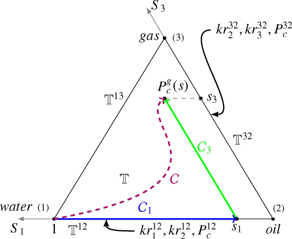
Illustration of the ternary diagram T and the location of the required two-phase data used in approach A.
Schéma du diagramme ternaire T et des données diphasiques requises dans l’approche A.
This TD equivalent condition yields two simple linear equations, which can be solved on the ternary diagram using (7) and the three-phase oil fractional flow f2. Therefore, we are able to build the global capillary function
| (9) |
Therefore, the global capillary function
| (10) |
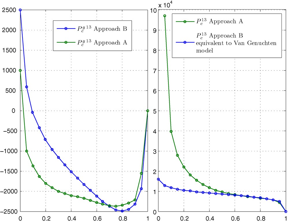
Following Chavent and Salzano (1985) and Chavent and Jaffré (1986), the next step determines d on the third side, that is, the water-gas side of T. The global mobility of the water-gas side d13must be determined carefully. Otherwise, corresponding relative permeabilities
At the end of the procedure, global mobility d(s,p), fractional flows fj(s,p) and global capillary function
3.2 New TD interpolation by finite elements (approach B)
In the exact global pressure formulation, d, f1, f2, f3, and
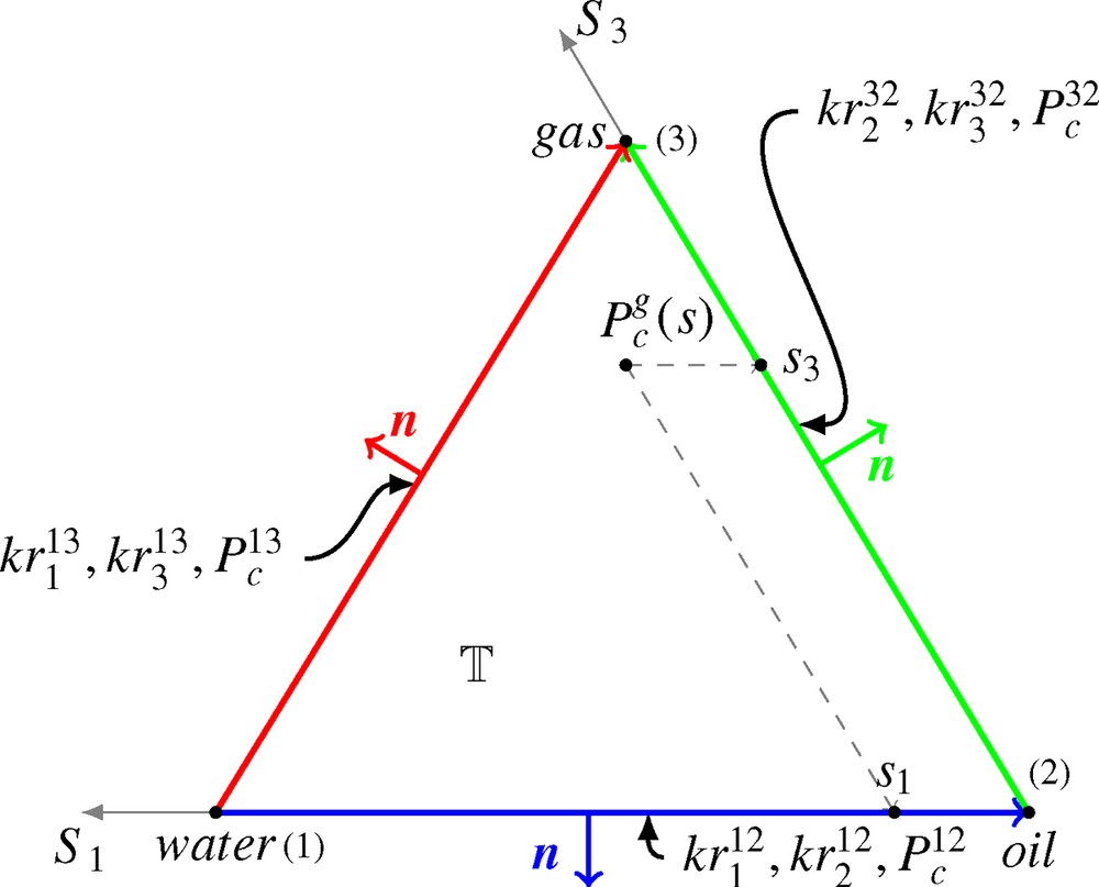
Illustration of the ternary diagram T and the location of the required two-phase data used in approach B.
Schéma du diagramme ternaire T et des données diphasiques requises dans l’approche B.
We solve first the initial value problems on the three two-phase sides of the ternary diagram T. The three ODEs are built up from tangential derivatives of
To satisfy the TD condition on the boundaries, the global capillary function must be slightly modified on the gas-oil side to provide an exact matching value at the gas vertex (Chavent, 2009; di Chiara Roupert, 2009; di Chiara Roupert et al., 2010).
The three two-phase global mobilities d on boundaries are then computed (see Eq. (7)) with P replaced by
In the last step, the global capillary pressure is extended to the entire ternary diagram T. It is necessary to complete the Dirichlet conditions known from ODE calculations with Neumann conditions along the same boundaries (see Fig. 2). Thus the problem amounts to enquire on each node the function
| (11) |
4 A comparison of numerically derived three-phase TD data
In this section, we compare the water fractional flow f1, the global mobility d and the global capillary pressure
Données initiales utilisées pour les trois systèmes diphasiques.
| Symbol | Value | Description | Unit |
| α | 0.0001 | α Van Genuchten parameter, fine sand | [Pa−1] |
| m | 0.93 | m Van Genuchten parameter, fine sand | [–] |
| μ 1 | 1.2 | Water dynamic viscosity | [×10−3Pa.s] |
| μ 2 | 0.55 | Oil dynamic viscosity | [×10−3Pa.s] |
| μ 3 | 0.015 | Gas dynamic viscosity | [×10−3Pa.s] |
| σ13/σ32 | 2.5 | Gas-oil dimensionless surface tension | [–] |
| σ13/σ12 | 2.1 | Water-oil dimensionless surface tension | [–] |
| B j | 1 | Volume factor for j = 1, 2, 3 | [–] |
| p | 1 | Global pressure level | [bar] |

Water fractional flow f1 obtained with approach A.
Flux fractionnaire en eau f1 obtenu suivant l’approche A.
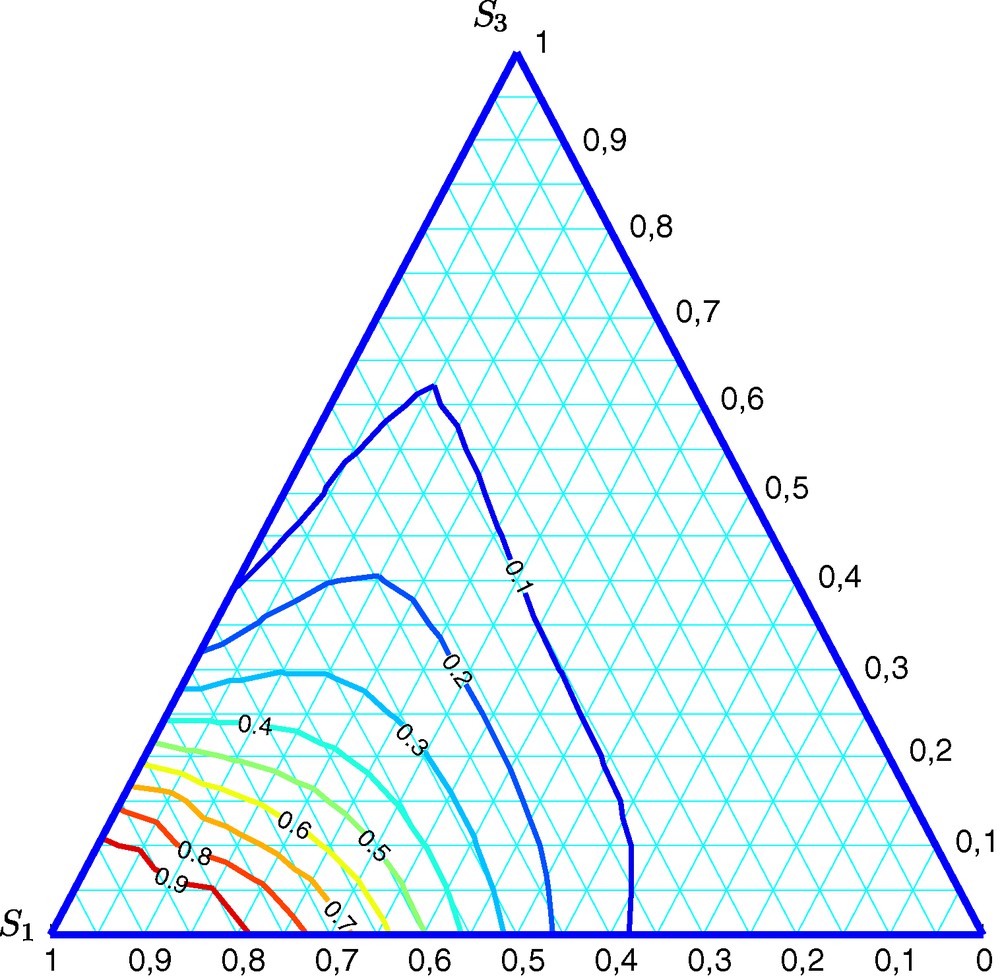
Water fractional flow f1 obtained with approach B.
Flux fractionnaire en eau f1 obtenu suivant l’approche B.
TD fractional flows computed from (11) exactly match the given initial models of two-phase capillary pressures and relative permeabilities (see Fig. 2). To compare both approaches, we calculated relative differences at the point of the ternary diagram at which s1 = 45% and s3 = 40%. At this point, the TD fractional flow obtained with approach A is about 25% higher than the one evaluated with approach B. In this case, the water volumetric flow vector (8) is higher in approach A than B. Figs. 5–7 show the global capillary function obtained from the optimization approach and the C1 finite element approach, respectively. Resulting values vary in the same range. One can see that the initial value
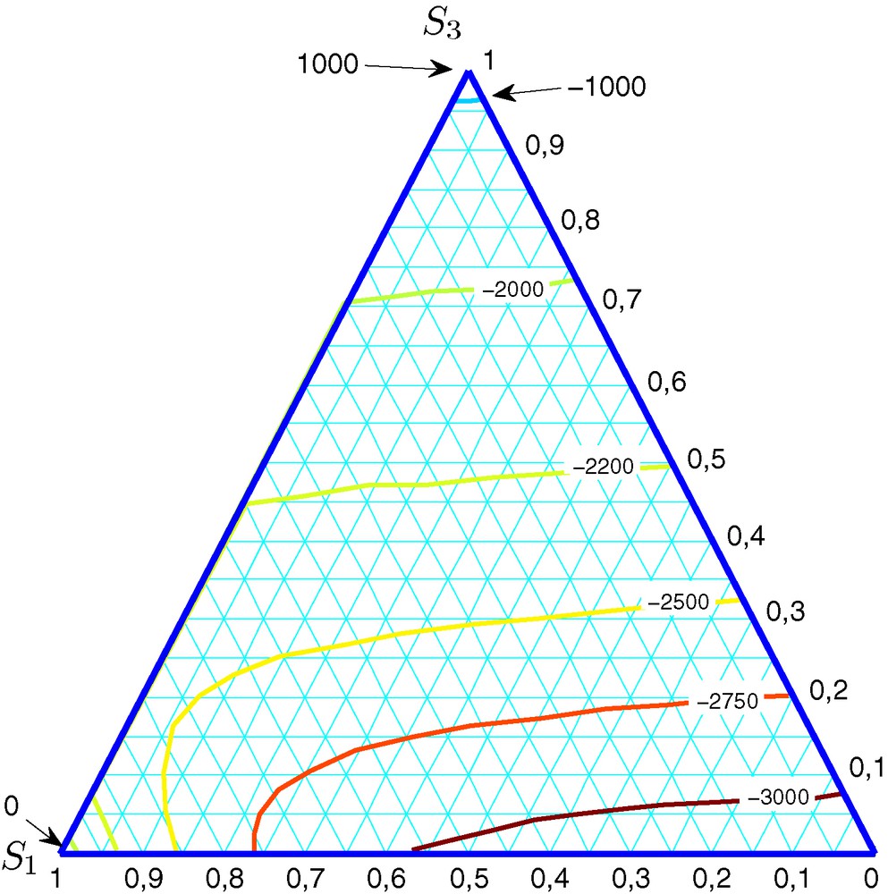
Global capillary pressure
Pression capillaire globale
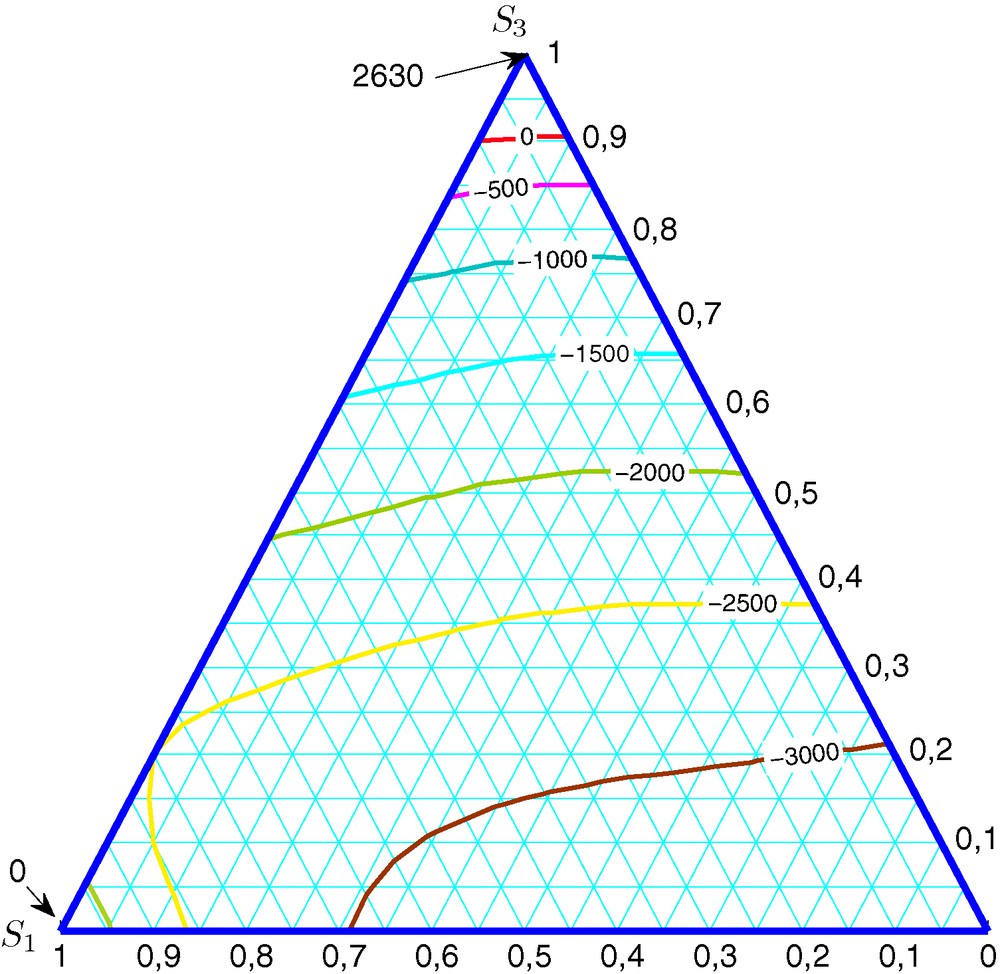
Global capillary pressure
Pression capillaire globale
Global capillary pressure
Pression capillaire globale
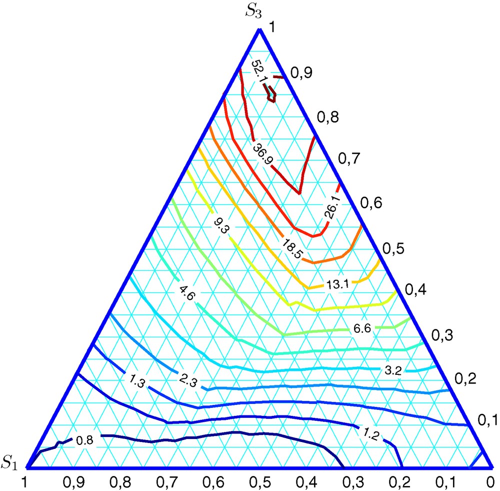
Global mobility d obtained with approach A.
Mobilité globale d obtenue suivant l’approche A.
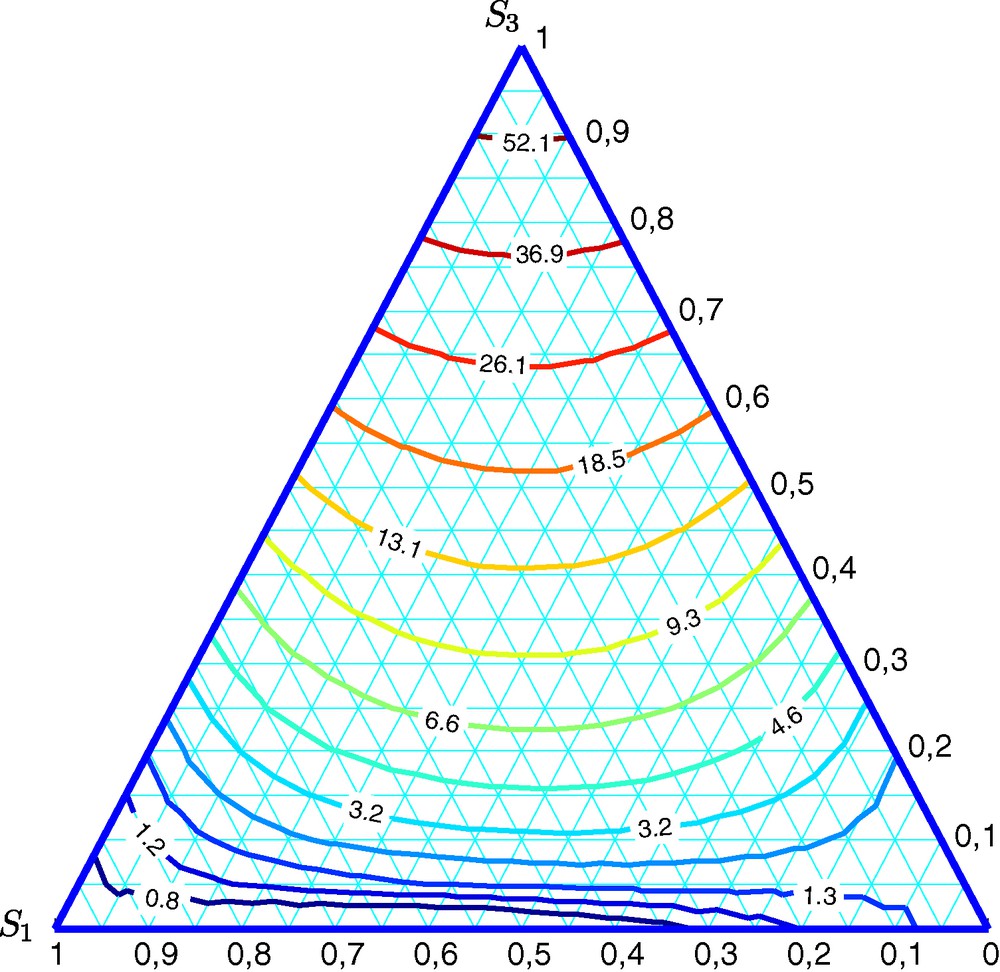
Global mobility d obtained with approach B.
Mobilité globale d obtenue suivant l’approche B.
5 Conclusion
In this article, we analysed two three-phase parameterisation approaches to assess the TD secondary variables required for efficient multiphase flow simulators using a global pressure formulation. Usually, experimental three-phase data are rarely investigated inside the three-phase water-oil-gas diagram (Bano et al., 2009; Oak et al., 1990). From a practical point of view, these two TD interpolations have given similar CPU times within the order of a second. They represent robust and innovative approaches for efficiently modelling three-phase flow equations. Both methods satisfy the TD condition and allow the three-phase compressible flow equation to be rewritten in a more suitable fractional form; see equations (6) and (8). However, by construction, the resulting two-phase water-gas data, such as the capillary pressure curve, differ between the original and the new TD interpolation. When flow takes place only in a two-phase water-gas system, TD three-phase data obtained by the optimization (approach A) might be significantly different from that derived using the finite element interpolation (approach B). It also may differ from the data from methods using classical capillary curves, such as the Van Genuchten model, as is often employed in the field of environmental sciences. As shown in Fig. 7, the finite element approach seems to be more suitable for explicitly taking into account two-phase capillary pressure and relative permeability data in a water-gas system. Furthermore, optimization parameters may be difficult to select. They depend on the governing parameters of the simulated cases (eg. viscosities, pressure levels, etc.) and more specifically initial values for the two relative permeability models used on the water-gas side optimization. Moreover, numerical tests (see approach A) showed that the global mobility field heavily depends on dynamic viscosity of the gas phase. Therefore, a finite element interpolation approach combined with a flow simulator seems to be better suited to generate three-phase flow variables than the optimization approach. In other words, the finite element approach appears to be a robust and efficient solution for three-phase flow simulation. At the reservoir scale, we can expect these differences to have little impact on the flow behaviour, as it is knwon that the shock saturation mainly dominates two phase flows. Note that in the TD approach, Chavent and Jaffré (1986) showed that the hyperbolicity condition is not fully verified particularly for large oil saturation values in the first Stone model. This condition should be satisfied by any three-phase data set if one wants small capillary pressure problems to be well posed for any values of volume factors. Besides, Stone's models are not TD compatible and therefore do not allow reformulation of the flow in a simplified way (see (6). Further research will be focussed on more systematic numerical flow comparisons with other three-phase correlations.
Acknowledgements
The authors would like to thank Professor Frédéric Delay from the University of Poitiers and the four other anonymous referees for their valuable comments and suggestions which helped improve the manuscipt significantly. Financial support for this research from the Programme National de Recherche en Hydrologie (INSU-CNRS) and the Agence De l’Environnement et de la Maîtrise de l’Energie (ADEME) is gratefully acknowledged. We would also like to thank ADEME and Burgéap SA for financing the PhD of R. di Chiara Roupert.