Fluctuation theory of ambient noise imaging

Josselin Garnier; George Papanicolaou

doi:10.1016/j.crte.2011.01.004

Internal geophysics/Applied geophysics

Fluctuation theory of ambient noise imaging
[Analyse des fluctuations pour l’imagerie par bruit ambiant]

Présenté par : Written on invitation of Editorial Board

Josselin Garnier ¹ ; George Papanicolaou ²

¹ Laboratoire de probabilités et modèles aléatoires et laboratoire Jacques-Louis Lions, université Paris VII, 75205 Paris cedex 13, France
² Mathematics Department, Stanford University, Stanford, CA 94304 United States

Comptes Rendus. Géoscience, Volume 343 (2011) no. 8-9, pp. 502-511.

Résumés

Anglais
Français

Travel time estimation and reflector imaging can be carried out using the cross correlations of signals generated by ambient noise sources and recorded at sensor arrays. We study here the mean and variance of the estimated quantities both with respect to the distribution of the noise sources and with respect to the distribution of the randomly scattering medium. In particular, we discuss the trade-off between resolution enhancement due to illumination diversification by scattering and the associated signal-to-noise ratio reduction, also due to scattering.

Il est possible d’estimer des temps de trajet et d’imager des réflecteurs, en utilisant les corrélations croisées de signaux émis par des sources de bruit ambiant et enregistrés par des réseaux de capteurs. Dans cette note, on étudie la moyenne et la variance de ces estimations vis-à-vis de la distribution des sources de bruit et vis-à-vis de la distribution du milieu aléatoire diffusant. En particulier on discute du compromis entre l’amélioration de la résolution et la réduction du rapport signal-sur-bruit, dues à la diffusion.

Métadonnées

Reçu le : 2010-08-30
Accepté le : 2011-01-25
Publié le : 2011-04-20

DOI : 10.1016/j.crte.2011.01.004

Keywords: Imaging, Seismic noise
Mot clés : Imagerie, Bruit sismique

Affiliations des auteurs :

Josselin Garnier ¹ ; George Papanicolaou ²

@article{CRGEOS_2011__343_8-9_502_0,
     author = {Josselin Garnier and George Papanicolaou},
     title = {Fluctuation theory of ambient noise imaging},
     journal = {Comptes Rendus. G\'eoscience},
     pages = {502--511},
     publisher = {Elsevier},
     volume = {343},
     number = {8-9},
     year = {2011},
     doi = {10.1016/j.crte.2011.01.004},
     language = {en},
}

TY  - JOUR
AU  - Josselin Garnier
AU  - George Papanicolaou
TI  - Fluctuation theory of ambient noise imaging
JO  - Comptes Rendus. Géoscience
PY  - 2011
SP  - 502
EP  - 511
VL  - 343
IS  - 8-9
PB  - Elsevier
DO  - 10.1016/j.crte.2011.01.004
LA  - en
ID  - CRGEOS_2011__343_8-9_502_0
ER  -

%0 Journal Article
%A Josselin Garnier
%A George Papanicolaou
%T Fluctuation theory of ambient noise imaging
%J Comptes Rendus. Géoscience
%D 2011
%P 502-511
%V 343
%N 8-9
%I Elsevier
%R 10.1016/j.crte.2011.01.004
%G en
%F CRGEOS_2011__343_8-9_502_0

Josselin Garnier; George Papanicolaou. Fluctuation theory of ambient noise imaging. Comptes Rendus. Géoscience, Volume 343 (2011) no. 8-9, pp. 502-511. doi : 10.1016/j.crte.2011.01.004. https://comptes-rendus.academie-sciences.fr/geoscience/articles/10.1016/j.crte.2011.01.004/

Version originale du texte intégral

1 Introduction

The Green's function of the wave equation in an inhomogeneous medium can be estimated by cross correlating signals emitted by ambient noise sources and recorded by a passive sensor array (Bardos et al., 2008; Colin de Verdière, 2009; Shapiro et al., 2005; Wapenaar and Fokkema, 2006; Weaver and Lobkis, 2001). The main result is that the cross correlation $C_{T} (τ, x_{1}, x_{2})$ of the signals u (t,x₁) and u (t,x₂), recorded at two sensors x₁ and x₂ defined by:

C_{T} (τ, x_{1}, x_{2}) = \frac{1}{T} \int_{0}^{T} u (t, x_{1}) u (t + τ, x_{2}) d t,

(1)

is related to the Green's function G(t,x₁,x₂) between x₁ and x₂. In a homogeneous medium and when the source of the waves is a space-time stationary random field that is delta correlated in space and time, it has been shown (Roux et al., 2005; Snieder, 2004) that the τ − derivative of the cross correlation of the recorded signals is proportional to the symmetrized Green's function between the sensors:

\partial_{τ} C_{T} (τ, x_{1}, x_{2}) \propto - [G (τ, x_{1}, x_{2}) - G (- τ, x_{1}, x_{2})] .

(2)

In an inhomogeneous medium and when the sources completely surround the region of the sensors the approximate identity (2) is still valid and it can be shown using the Helmholtz-Kirchhoff theorem (Garnier and Papanicolaou, 2009; Schuster, 2009; Wapenaar and Fokkema, 2006). This is true even with spatially localized noise source distributions provided the waves propagate within an ergodic cavity (Bardos et al., 2008). To summarize, when the ambient noise sources are well distributed around the sensors, the cross correlation as a function of the lag time τ has a peak at plus or minus the inter-sensor travel time

τ_{x_{1}, x_{2}}

. However, when the ambient noise sources have spatially limited support, the recorded signals are generated by wave energy flux coming from the direction of the noise sources, which results in an azimuthal dependence of travel time estimation process (Stehly et al., 2006). In general, travel time estimation by cross correlation of noise signals is possible when the line between the sensors is along the direction of the energy flux and difficult or impossible when it is perpendicular to it. This can be explained using a stationary phase analysis (Garnier and Papanicolaou, 2009; Godin, 2009; Snieder, 2004) and we present this result in Section 3.1. It is, however, possible to enhance the quality of travel time estimation by exploiting the enhanced directional diversity provided by the scattering of waves in a randomly scattering medium (Garnier and Papanicolaou, 2009; Stehly et al., 2008). We present and analyze this idea in Section 3.3.

Cross correlations of signals emitted by ambient noise sources and recorded by a passive sensor array can also be used for imaging of reflectors imbedded in the medium (Garnier and Papanicolaou, 2009, 2010; Gouédard et al., 2008). The data that is used for imaging is the cross correlation matrix ${(C (τ, x_{j}, x_{l}))}_{j, l = 1, \dots, N}$ between pairs of sensors of the passive array (x_j)_{j = 1,...,N}. In Section 4 we consider imaging functionals that use the cross correlation matrix to image the reflectors. The forms of these functionals are motivated by the analysis of the cross correlation matrix in the asymptotic regime where the coherence time of the sources is smaller than the typical travel times to be estimated and used. The imaging functionals can then be applied in general, in a smooth or randomly scattering medium.

For travel time estimation and reflector imaging we pay particular attention to the statistical stability of the estimation. There are two types of statistical stability in these problems:

• First there is the issue of statistical stability with respect to the distribution of the noise sources. This means that the empirical cross correlation C_T depends on the realizations of the signals generated by the ambient noise sources. However C_T is self-averaging (or statistically stable) in the sense that the time average in (1) over an interval of duration T tends to a statistical average when T is large enough, as shown in Section 2. Therefore, statistical stability relative to the distribution of the noise sources can be controlled through the choice of a long enough recording time-window or by stacking techniques;
• Second there is the issue of statistical stability with respect to the distribution of the scattering medium. This means that the cross correlation depends on the realization of the randomly scattering medium. It is not in general a self-averaging quantity. Indeed we will see in this note that fluctuations of the cross correlation due to the randomly scattering medium can have a large standard deviation that depends on the spectrum of the noise sources and on statistical properties of the scattering medium. Furthermore, statistical stability with respect to the distribution of the random medium cannot be controlled in general. In Sections 3.2 and 4.3 we analyze the trade-off between resolution enhancement and signal-to-noise ratio (SNR) reduction due to scattering by a random medium. We show in Section 3.3 and 4.4 that the use of iterated cross correlations can improve the SNR. We also carry out some simple numerical simulations to illustrate the results. They confirm that the theoretical predictions obtained by asymptotic analysis can be seen in realistic configurations.

2 Stability with respect to the noise source distribution

We consider the solution u of the scalar wave equation in a three-dimensional smooth medium with speed of propagation c(x):

\frac{1}{c^{2} (x)} \frac{\partial^{2} u}{\partial t^{2}} - Δ_{x} u = n (t, x) .

(3)

The term n(t,x) models a random field of noise sources. It is a zero-mean stationary (in time) random process with autocorrelation function

< n (t_{1}, y_{1}) n (t_{2}, y_{2}) > = F (t_{2} - t_{1}) K (y_{1}) δ (y_{1} - y_{2}) .

(4)

Here < > stands for statistical average with respect to the distribution of the noise sources. For simplicity we consider that the process n has Gaussian statistics.

The time distribution of the noise sources is characterized by the correlation function F(t₂–t₁), which is a function of t₂–t₁ only by time stationarity. The Fourier transform $\hat{F} (ω)$ of the time correlation function F(t) is a nonnegative, even, real-valued function proportional to the power spectral density of the sources (Bochner's theorem):

\hat{F} (ω) = \int F (t) e^{i ω t} d t .

(5)

The spatial distribution of the noise sources is characterized by the autocovariance function δ(y₁ − y₂)K(y₁). The process n is delta-correlated in space and K characterizes the spatial support of the sources. It is possible to consider a more general form for the spatial autocovariance function (Bardos et al., 2008). The analysis then requires the use of semi-classical methods but the results do not change qualitatively.

We denote by G(t,x,y) the time-dependent outgoing Green's function. It is the fundamental solution of the wave equation

\frac{1}{c^{2} (x)} \frac{\partial^{2} G}{\partial t^{2}} - Δ_{x} G = δ (t) δ (x - y),

(6)

starting from G(0, x, y) = ∂_tG(0, x, y) = 0 (and continued on the negative time axis by G(t, x, y) = 0, ∀t ≤ 0). When the medium is homogeneous with speed of propagation c₀, the time-dependent Green's function G(t, x, y) = A_x,yδ(t − T_x,y) where A_x,y = 1/(4π|x − y|) and T_x,y = |x − y|/c₀ is the travel time.

The empirical cross correlation of the signals recorded at x₁ and x₂ for an integration time T is defined by (1). It is a statistically stable quantity, in the sense that for a large integration time T, the empirical cross correlation C_T is independent of the realization of the noise sources. We have the following results (the first two items are proved in Garnier and Papanicolaou, 2009):

• The expectation of the empirical cross correlation C_T (with respect to the distribution of the sources) is independent of T:

< C_{T} (τ, x_{1}, x_{2}) > = C^{(1)} (τ, x_{1}, x_{2}),

(7)

where the statistical cross correlation C⁽¹⁾ is given by

C^{(1)} (τ, x_{1}, x_{2}) = \frac{1}{2 π} \int [\int \bar{\hat{G}} (ω, x_{1}, y) \hat{G} (ω, x_{2}, y) K (y) d y] \times \hat{F} (ω) e^{- i ω τ} d ω,

(8)

and

\hat{G} (ω, x, y)

is the time-harmonic Green's function (i.e. the Fourier transform of G(t, x, y)).

• The empirical cross correlation C_T is a self-averaging quantity:

C_{T} (τ, x_{1}, x_{2}) \overset{T \to \infty}{\to} C^{(1)} (τ, x_{1}, x_{2}),

(9)

in probability with respect to the distribution of the sources.

• The covariance of the empirical cross correlation C_T is:

C o v (C_{T} (τ, x_{1}, x_{2}), C_{T} (τ + Δ τ, x_{1}, x_{2})) = \frac{1}{2 π T} \int [\int \bar{\hat{G}} (ω, x_{1}, y) \hat{G} (ω, x_{2}, y) K (y) d y]^{2} \hat{F} {(ω)}^{2} e^{- i ω (2 τ + Δ τ)} d ω + \frac{1}{2 π T} \int [\int | \hat{G} (ω, x_{1}, y) |^{2} K (y) d y] [\int | \hat{G} (ω, x_{2}, y) |^{2} K (y) d y] \hat{F} {(ω)}^{2} e^{- i ω Δ τ} d ω,

(10)

when BT ≫ 1 (here B is the bandwidth of the noise sources). The first term in the right-hand side of (10) is of the same form as the square of the expectation, but the second term of the right-hand side is different. When the medium is homogeneous with speed of propagation c₀ and the distance from the source region (assumed here to be localized) to the sensors is L, then the variance of the fluctuations can be approximated by

V a r (C_{T} (τ, x_{1}, x_{2})) \approx \frac{1}{2^{9} π^{5} T L^{4}} {[\int K (y) d y]}^{2} \int \hat{F} {(ω)}^{2} d ω .

(11)

This shows that:

• all noise sources participate in the fluctuations of the empirical cross correlation (since the volume integral of the source function K appears in (11));
• the standard deviation of the fluctuations decays as (BT)^–1/2 (the square root of the integration time T times the noise bandwidth B) and as L^–2 (the square distance from the sources to the sensors).

Therefore errors may occur when the averaging time is not sufficient to ensure that time averages approximate statistical mean values (Gouédard et al., 2008). However, the integration time is usually not a limiting factor, therefore this error can be brought to an arbitariliy small value and we will neglect it in the following.

3 Travel time estimation

If we consider the expression (8) of the cross correlation when the noise sources surround the region of interest that contains the sensors, then the term in the square brackets can be computed by the Helmholtz-Kirchhoff identity: this identity yields that this term is proportional to the imaginary part of the Green's function and we then find that the derivative of the cross correlation is proportional to the symmetrized Green's function convoluted with the time correlation function of the noise sources (Garnier and Papanicolaou, 2009, Section 4.4):

\partial_{τ} C_{T} (τ, x_{1}, x_{2}) \propto - F * [G (\cdot, x_{1}, x_{2}) - G (- \cdot, x_{1}, x_{2})] (τ) .

(12)

Travel time estimation is then straightforward as the singular component of the Green's function G(τ, x₁, x₂) is concentrated at time lag τ equal to the travel time $T_{x_{1}, x_{2}}$ . When the noise sources are spatially localized the Helmholtz-Kirchhoff identity cannot be used and we address in this section travel time estimation in this situation.

3.1 Analysis in the high-frequency regime

We assume from now on that the decoherence time of the noise sources is much smaller than the typical travel time that we want to estimate. If we denote by ɛ the (small) ratio of these two time scales, then we can write the time correlation function F_ɛ of the noise sources in the form

F_{ε} (t_{2} - t_{1}) = F (\frac{t_{2} - t_{1}}{ε}),

(13)

where t₁ and t₂ are scaled relative to typical travel times. The hypothesis ɛ ≪ 1 is both natural and useful:

• in applications, such as surface wave tomography, noise records are first bandpass-filtered and then cross correlated (Shapiro et al., 2005). If the central frequency ω₀ of the filter is high enough so that the corresponding wavelength λ₀ is much smaller than the typical travel distance d, then we have ɛ = λ₀/d ≪ 1. As we will see below, the resolution by cross correlation is inversely proportional to the bandwidth, so the hypothesis ɛ ≪ 1 turns out to be natural in order to get some resolution (i.e. an estimate of the travel time with an accuracy smaller than the total travel time through the region);
• the Fourier transform of the time correlation function of the sources has the form ${\hat{F}}_{ε} (ω) = ε \hat{F} (ε ω)$ , so that the cross correlation (8) involves a product of Green's functions evaluated at high frequencies:
$C^{(1)} (τ, x_{1}, x_{2}) = \frac{1}{2 π} \iint \hat{F} (ω) K (y) \bar{\hat{G}} (\frac{ω}{ε}, x_{1}, y) \hat{G} (\frac{ω}{ε}, x_{2}, y) e^{- i ω \frac{τ}{ε}} d y d ω$ (14)

When ɛ ≪ 1 we can use a geometric asymptotics approximation for the Green's function

\hat{G} (\frac{ω}{ε}, x, y) ≃ A_{x, y} \exp (i \frac{ω}{ε} T_{x, y}),

(15)

and we find that the expression (14) has the form of a multiple integral with a smooth amplitude and a rapid phase. Therefore, a stationary phase analysis appears as an appropriate tool to study the cross correlations in the regime ɛ ≪ 1. For simplicity we assume in the following that the background medium is homogeneous with speed of propagation c₀. Then A_x,y = 1/(4π|x − y|) and T_x,y = |x − y|/c₀. Using stationary phase arguments one obtains the following expression for the cross correlation in the regime ɛ small:

\partial_{τ} C^{(1)} (τ, x_{1}, x_{2}) = \frac{c_{0}}{2} A_{x_{1}, x_{2}} [K_{x_{2}, x_{1}} F_{ε} (τ + T_{x_{1}, x_{2}}) - K_{x_{1}, x_{2}} F_{ε} (τ - T_{x_{1}, x_{2}})],

(16)

where

K_{x_{1}, x_{2}}

is the power released by the noise sources located along the ray starting from x₁ with the direction of x₁–x₂ (it is a piece of the ray joining x₁ and x₂):

K_{x_{1}, x_{2}} = \int_{0}^{\infty} K (x_{1} + \frac{x_{1} - x_{2}}{| x_{1} - x_{2} |} l) d l .

(17)

Note that $K_{x_{1}, x_{2}}$ is not zero only if the ray starting from x₂ and going through x₁ extends into the source region. In other words, sources located along the ray starting from x₁ with the direction of x₁–x₂ (resp. x₂–x₁) give rise to a singular component at $τ = T_{x_{1}, x_{2}}$ (resp. $τ = - T_{x_{1}, x_{2}}$ ). In Fig. 1a–b one can see a peak at $τ = T_{x_{1}, x_{j}}$ because the ray going through x₁ and x_j intersects the source region. In Fig. 1c–d one cannot see any peak at $τ = \pm T_{x_{1}, x_{j}}$ because the ray going through x₁ and x_j does not intersect the source region.

Fig. 1
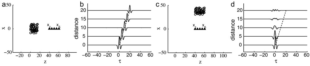
Travel time estimation in a homogeneous medium. The first configuration is plotted in Figure (a): the circles are the noise sources and the triangles are the sensors. Figure (b) plots the cross correlation C⁽¹⁾ between the pairs of sensors (x₁,x_j), j = 1,...,5, versus the distance $|x_{j} - x_{1}|$ . The second configuration is plotted in Figure (c) and Figure (d) plots the corresponding cross correlation C⁽¹⁾. Here $\hat{F} (ω) = ω^{2} \exp (- ω^{2})$ and c₀ = 1.
Estimation des temps de trajet dans un milieu homogène. La figure (a) est une esquisse de la première situation: les cercles sont les sources de bruit et les triangles sont les capteurs. La corrélation croisée C⁽¹⁾ entre les paires de capteurs (x₁,x_j), j = 1,...,5, est dessinée en fonction de la distance $|x_{j} - x_{1}|$ dans la figure (b). La figure (c) est une esquisse de la seconde situation et la figure (d) dessine la corrélation croisée correspondante. Ici $\hat{F} (ω) = ω^{2} \exp (- ω^{2})$ et c₀ = 1.

To summarize, when ɛ is small, the cross correlation C⁽¹⁾(τ, x₁, x₂) has singular components (at $τ = \pm T_{x_{1}, x_{2}}$ ) if and only if the ray going through x₁ and x₂ reaches into the source region, that is, into the support of the function K. The results (16), (17) also show that:

• only the noise sources located in a small tube around the ray joining x₁ and x₂ contribute to the singular components of C⁽¹⁾(τ, x₁, x₂) (this can be seen from the line integral (17));
• the widths of the peaks are determined by the bandwidth of the noise sources;
• the heights of the peaks do not depend on the distance from the sources to the sensor array.

This last property follows from the stationary phase analysis and is a consequence of two competing phenomena that cancel each other: on the one hand the geometric decay of the amplitude of the Green's function as a function of the distance from the sources to the sensors, and on the other hand the increase of the diameter of the small tube around the ray that contributes to the singular components.

3.2 Signal-to-noise ratio reduction and enhanced resolution due to scattering

In order to analyze the cross correlation technique in a scattering medium, we first introduce a model for the inhomogeneous medium. We assume that the medium has a homogeneous background speed c₀ and small and weak fluctuations responsible for scattering:

\frac{1}{c^{2} (x)} = \frac{1}{c_{0}^{2}} [1 + V (x)],

where V(x) is a random process with mean zero and covariance function of the form

E [V (x) V (x^{'})] = σ_{s}^{2} l_{s}^{3} ρ (x) δ (x - x^{'}) .

Here E stands for the expectation with respect to the distribution of the randomly scattering medium, σ_s is the standard deviation of the fluctuations of the speed of propagation, l_s is the correlation length of the fluctuations, and the function ρ(x) characterizes the spatial support of the scattering region. Note that we have assumed that the correlation length is small enough so that we can consider that the process V is delta-correlated.

To leading order in the scattering strength the average cross correlation is the sum of the unperturbed cross correlation $C_{0}^{(1)}$ (i.e. the cross correlation (8) in the absence of scattering) and of an additional term of the form:

E [C^{(1)} (τ, x_{1}, x_{2})] - C_{0}^{(1)} (τ, x_{1}, x_{2}) = \frac{1}{2 π} \iint ω^{4} {\hat{F}}_{ε} (ω) K^{ρ} (y) \bar{\hat{G}} (ω, x_{1}, y) \hat{G} (ω, x_{2}, y) e^{- i ω τ} d y d ω,

(18)

where

K^{ρ} (z) = ρ (z) \frac{σ_{s}^{2} l_{s}^{3}}{2^{4} π^{2} c_{0}^{4}} \int \frac{K (y)}{| y - z |^{2}} d y .

(19)

Note that the support of the function K^ρ is the support of ρ, i.e. the scattering region. K^ρ(z) is proportional to the total power reemitted from z by scattering. Eq. (18), which has the same form as (8) but with K^ρ instead of K, shows that the random scatterers play the role of secondary sources. The average cross correlation (18) possesses additional peaks at $τ = T_{x_{1}, x_{2}}$ (resp. $τ = - T_{x_{1}, x_{2}}$ ) due to the scattered waves provided that there are rays issued from the scattering region that goes through x₁ and then x₂ (resp. through x₂ and then x₁). Indeed in the high-frequency regime we find

E [\partial_{τ} C^{(1)} (τ, x_{1}, x_{2})] - \partial_{τ} C_{0}^{(1)} (τ, x_{1}, x_{2}) = \frac{c_{0}}{2} A_{x_{1}, x_{2}} [K_{x_{2}, x_{1}}^{ρ} F_{ε}^{(4)} (τ + T_{x_{1}, x_{2}}) - K_{x_{1}, x_{2}}^{ρ} F_{ε}^{(4)} (τ - T_{x_{1}, x_{2}})],

(20)

where

K_{x_{1}, x_{2}}^{ρ}

is defined as in (17) but in terms of K^ρ instead of K, and

F_{ε}^{(4)}

is the fourth-order derivative of F_ɛ. This shows that:

• all noise sources but only the scatterers along the ray joining x₁ and x₂ participate in the additional peaks;
• the heights of the additional peaks decay with the square distance from the sources to the scattering region.

To leading order in the scattering strength and in the high-frequency regime, we find using again stationary phase arguments that the variance of the fluctuations of the cross correlation is:

\int V a r (\partial_{τ} C^{(1)} (τ, x_{1}, x_{2})) d τ = \frac{σ_{s}^{2} l_{s}^{3}}{2^{11} π^{5} c_{0}^{2}} [\int ω^{4} {\hat{F}}_{ε} {(ω)}^{2} d ω] \int ρ (z) \frac{{(K_{z, x_{1}} - K_{z, x_{2}})}^{2} + K_{x_{1}, z}^{2} + K_{x_{2}, z}^{2}}{| z - x_{1} |^{2} | z - x_{2} |^{2}} d z .

(21)

This shows that:

• all noise sources and all scatterers participate in the fluctuations of the cross correlation due to the randomly scattering medium (and not only the ones along a particular ray);
• the standard deviation of the fluctuations decay with the square distance from the sources to the scattering region and with the square distance from the scattering region to the sensors;
• in terms of the noise bandwidth B, the standard deviation scales as B^1/2 while the amplitudes of the peaks scale as B, which shows that the relative fluctuations decay with the bandwidth.

The analysis of the mean and variance of C⁽¹⁾ therefore shows that scattering can enhance the directional diversity of the wave fields recorded by the sensors, which can help in travel time estimation, but it also increases the fluctuations of the cross correlation, which may make the additional peaks difficult to detect. The use of fourth-order cross correlations discussed in the next subsection is a way to increase the SNR of travel time estimation in randomly scattering media.

3.3 Use of fourth-order cross correlations

It is possible to estimate the travel time between two sensors x₁ and x₂ in a scattering medium by looking at the main peaks of a special fourth-order cross correlation $C_{T}^{(3)} (τ, x_{1}, x_{2})$ (C⁽³⁾ stands for Correlation of Coda of Correlation) (Stehly et al., 2008). This fourth-order cross correlation uses the data recorded by an array of auxiliary sensors x_a,k, k = 1,...,N_a, and it is evaluated as follows:

• calculate the cross correlations between x₁ and x_a,k and between x₂ and x_a,k for each auxiliary sensor x_a,k as in (1);
• calculate the coda (i.e. the tails) of these cross correlations:
$C_{T, c o d a} (τ, x_{a, k}, x_{l}) = C_{T} (τ, x_{a, k}, x_{l}) 1_{[T_{c 1}, T_{c 2}]} (| τ |), for l = 1,2, k = 1, \dots, N_{a};$
• cross correlate the tails of the cross correlations and sum them over all auxiliary sensors to form the coda cross correlation between x₁ and x₂:
$C_{T}^{(3)} (τ, x_{1}, x_{2}) = \sum_{k = 1}^{N_{a}} \int C_{T, c o d a} (τ^{'}, x_{a, k}, x_{1}) C_{T, c o d a} (τ^{'} + τ, x_{a, k}, x_{2}) d τ^{'} .$

This algorithm is parameterized by three important times:

• the time T is the integration time and it should be large so as to ensure statistical stability with respect to the distribution of the noise sources;
• the time T_c1 should be large enough so that the Green's functions ${(G (t, x_{a, k}, x_{1}))}_{t \in [T_{c 1}, T_{c 2}]}$ and ${(G (t, x_{a, k}, x_{2}))}_{t \in [T_{c 1}, T_{c 2}]}$ limited to [T_c1,T_c2] do not contain the contributions of the direct waves. This means that T_c1 depends on the index of the auxiliary sensor k and should be a little bit larger than $\max (T_{x_{a, k}, x_{1}}, T_{x_{a, k}, x_{2}})$ ;
• the time T_c2 should be large enough so that the Green's functions ${(G (t, x_{a, k}, x_{1}))}_{t \in [T_{c 1}, T_{c 2}]}$ and ${(G (t, x_{a, k}, x_{2}))}_{t \in [T_{c 1}, T_{c 2}]}$ limited to [T_c1,T_c2] contain the contributions of the incoherent scattered waves. This means that T_c2 should be of the order of the power delay spread.

The coda cross correlation $C_{T}^{(3)}$ is a self-averaging quantity and it is equal to the statistical coda cross correlation C⁽³⁾ as T → ∞:

C^{(3)} (τ, x_{1}, x_{2}) = \sum_{k = 1}^{N_{a}} \int \bar{{\hat{C}}_{c o d a}^{(1)}} (ω, x_{a, k}, x_{1}) {\hat{C}}_{c o d a}^{(1)} (ω, x_{a, k}, x_{2}) e^{- i ω τ} d ω,

C_{c o d a}^{(1)} (τ, x_{a, k}, x_{l}) = C^{(1)} (τ, x_{a, k}, x_{l}) 1_{[T_{c 1}, T_{c 2}]} (| τ |) .

The coda cross correlation C⁽³⁾ differs from the cross correlation C⁽¹⁾ in that the contributions of the direct waves are eliminated and only the contributions of the scattered waves are taken into account (note that some of the contributions of scattered waves are also eliminated, but only those which correspond to small additional travel times, which are also those which induce small directional diversity). Since scattered waves have more directional diversity than the direct waves when the noise sources are spatially localized, the coda cross correlation C⁽³⁾(τ, x₁, x₂) usually exhibits a stronger peak at lag time equal to the inter-sensor travel time $T_{x_{1}, x_{2}}$ (Garnier and Papanicolaou, 2009). In particular, in contrast with the cross correlation C⁽¹⁾, the existence of a singular component at lag time equal to the travel time $T_{x_{1}, x_{2}}$ does not require that the ray joining x₁ and x₂ reaches into the source region, but only into the scattering region.

We illustrate these results in Fig. 2 in which the five sensors are aligned perpendicularly to the energy flux coming from the noise sources and the cross correlation C⁽¹⁾(τ, x₁, x_j) does not have a peak at lag time equal to the travel time between the sensors x₁ and x_j, j = 1,...,5. However the ray going through the sensors x₁ and x_j intersects the scattering region and the coda cross correlation C⁽³⁾(τ, x₁, x_j) has a peak at lag time equal to the travel time between the sensors. The comparison between Fig. 2c, d also shows that the auxiliary sensors are necessary to get the peak of the coda cross correlation.

Fig. 2
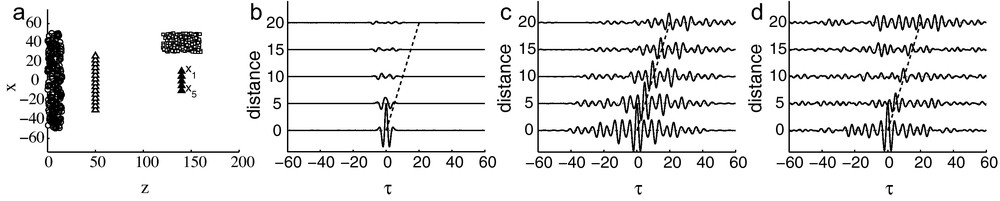
Travel time estimation in a scattering medium. The configuration is plotted in Figure (a): the circles are the noise sources, the squares are the scatterers, the triangles are the sensors, and the empty triangles are the auxiliary sensors. Figure (b) plots the cross correlation C⁽¹⁾ between the pairs of sensors (x₁,x_j), j = 1,...,5, versus the distance $|x_{j} - x_{1}|$ . Figure (c) plots the coda cross correlation C⁽³⁾ between the pairs of sensors when the auxiliary sensors are used. Figure (d) plots the coda cross correlation C⁽³⁾ when the auxiliary sensors are not used.
Estimation de temps de trajet dans un milieu diffusant. La figure (a) est une esquisse de la situation: les cercles sont les sources de bruit, les carrés sont les diffuseurs, les triangles pleins sont les capteurs et les triangles vides sont les capteurs auxiliaires. La corrélation croisée C⁽¹⁾ entre les paires de capteurs (x₁,x_j), j = 1,...,5, est dessinée en fonction de la distance $|x_{j} - x_{1}|$ dans la figure (b). La figure (c) dessine la corrélation croisée C⁽³⁾, lorsque les capteurs auxiliaires sont utilisés, et la figure (d) dessine la corrélation croisée C⁽³⁾, lorsque les capteurs auxiliaires ne sont pas utilisés.

4 Reflector imaging

In this section we show that cross correlations of signals emitted by ambient noise sources and recorded by a sensor array can also be used for imaging of reflectors. The data to be used for imaging is the matrix of cross correlations ${(C (τ, x_{j}, x_{l}))}_{j, l = 1, \dots, N}$ between pairs of sensors of an array ${(x_{j})}_{j = 1, \dots, N}$ . The objective is to image the reflectors buried in the medium. Here we consider the case in which there is only one reflector located at z_r. Note that it is often necessary to have available data sets ${(C (τ, x_{j}, x_{l}))}_{j, l = 1, \dots, N}$ and ${(C_{0} (τ, x_{j}, x_{l}))}_{j, l = 1, \dots, N}$ , with and without the reflector, respectively, so that we can compute the differential cross correlations ΔC = C − C₀ and migrate them. In general, but not always, the primary data set C cannot be used directly for imaging because peaks in the cross correlations due to the reflector may be very weak compared both to the peaks of the direct waves, at lag times equal to the inter-sensor travel times, as well as to the non-singular components due to the directionality of the energy flux (Garnier and Papanicolaou, 2009). In many applications where we want to image localized changes in the environment, such as in reservoir or volcano monitoring, both data sets are usually available.

4.1 Analysis in the high-frequency regime

By a stationary phase analysis and a Born approximation for the reflector the singular components of the differential cross correlations C⁽¹⁾(τ, x₁, x₂) can be identified (Garnier and Papanicolaou, 2010). This is important because this information will in turn allow us to determine the appropriate imaging functional that should be used to migrate the cross correlations. There are two main types of configurations of sources, sensors, and reflectors:

• the noise sources are spatially localized and the sensors are between the sources and the reflectors (Fig. 3a). We call this the daylight illumination configuration. In this configuration the singular components of the differential cross correlation are concentrated at lag times equal to (plus or minus) the sum of travel times $T_{x_{2}, z_{r}} + T_{x_{1}, z_{r}}$ ;
• the noise sources are spatially localized and the reflectors are between the sources and the sensors (Fig. 4a). We call this the backlight illumination configuration. In this configuration the singular components of the differential cross correlation are concentrated at lag times equal to the difference of travel times $T_{x_{2}, z_{r}} - T_{x_{1}, z_{r}}$ .

Fig. 3
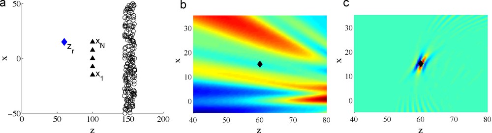
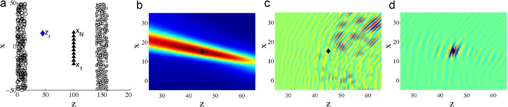
Passive sensor imaging in a homogeneous medium. The daylight illumination configuration is plotted in Figure (a): the circles are the noise sources, the triangles are the sensors, and the diamond is the reflector. Figure (b) plots the image obtained with the backlight imaging functional (25). Figure (c) plots the image obtained with the daylight imaging functional (24).
Imagerie passive dans un milieu homogène. La figure (a) est une esquisse de la situation: les cercles représentent les sources de bruit, les triangles sont les capteurs, et le losange représente le réflecteur. La figure (b) est l’image obtenue avec la fonction (25). La figure (c) est l’image obtenue avec la fonction (24).

Fig. 4
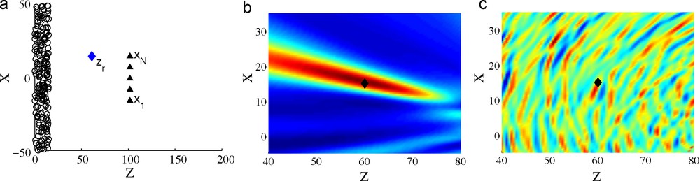
Passive sensor imaging in a homogeneous medium. The backlight illumination configuration is plotted in Figure (a). Figure (b) plots the image obtained with the backlight imaging functional (25). Figure (c) plots the image obtained with the daylight imaging functional (24).
Imagerie passive dans un milieu homogène. La figure (a) est une esquisse de la situation. La figure (b) est l’image obtenue avec la fonction (25). La figure (c) est l’image obtenue avec la fonction (24).

In the backlight imaging configuration, when ɛ is small, the differential cross correlation ΔC⁽¹⁾ has a unique singular contribution at lag time equal to the difference of travel times $T_{x_{2}, z_{r}} - T_{x_{1}, z_{r}}$ and it has the form:

Δ C^{(1)} (τ, x_{1}, x_{2}) = \frac{σ_{r} l_{r}^{3}}{32 π^{2} c_{0}} \frac{K_{z_{r}, x_{1}} - K_{z_{r}, x_{2}}}{| z_{r} - x_{1} | | z_{r} - x_{2} |} \partial_{τ} F_{ε} (τ - [T_{x_{2}, z_{r}} - T_{x_{1}, z_{r}}]),

(22)

where K_z,x is defined by (17). In the daylight illumination configuration, the differential cross correlation ΔC⁽¹⁾ has two singular contributions at lag times equal to plus or minus the sum of travel times

T_{x_{2}, z_{r}} + T_{x_{1}, z_{r}}

and it has the form:

Δ C^{(1)} (τ, x_{1}, x_{2}) = \frac{σ_{r} l_{r}^{3}}{32 π^{2} c_{0}} \frac{K_{x_{1}, z_{r}}}{| z_{r} - x_{1} | | z_{r} - x_{2} |} \partial_{τ} F_{ε} (τ - [T_{x_{2}, z_{r}} + T_{x_{1}, z_{r}}])

- \frac{σ_{r} l_{r}^{3}}{32 π^{2} c_{0}} \frac{K_{x_{2}, z_{r}}}{| z_{r} - x_{1} | | z_{r} - x_{2} |} \partial_{τ} F_{ε} (τ + [T_{x_{2}, z_{r}} + T_{x_{1}, z_{r}}]) .

(23)

Note that $K_{z_{r}, x_{j}}$ is not zero only if the ray going from x_j to z_r extends into the source region, which is the backlight illumination configuration, while $K_{x_{j}, z_{r}}$ is not zero only if the ray going from z_r to x_j extends into the source region, which is the daylight illumination configuration. Eq. (23) shows that:

• only the sources located along the rays joining x_j and z_r contribute to the singular components;
• the widths of the peaks are determined by the bandwidth of the noise sources;
• the heights of the peaks are inversely proportional to the square of the distance from the reflector to the sensor array, and they do not depend on the distance from the sources to the reflector or the sensor array.

4.2 Migration of cross correlations

As shown in the previous subsection, the cross correlation may have additional peaks at lag times that depend on the reflector location. This suggests that the reflector can be imaged by migrating the cross correlation matrix. This form of passive sensor array imaging depends in an essential way on the illumination configuration, that is, the relative positions of the sensors, the noise sources, and the reflector.

To form an image in a daylight illumination configuration (Fig. 3a), we propose to use the daylight imaging functional defined for a search point z^S in the image domain by:

I^{D} (z^{S}) = \sum_{j, l = 1}^{N} Δ C (T_{z^{S}, x_{l}} + T_{z^{S}, x_{j}}, x_{j}, x_{l}) .

(24)

This functional is built by evaluating each element of the cross correlation matrix at lag time equal to the sum of the travel times $T_{z^{S}, x_{l}} + T_{z^{S}, x_{j}}$ and by summing the migrated matrix elements over all pairs of sensors (it is therefore a Kirchhoff-type migration functional for the cross correlation matrix). The resolution analysis of the daylight imaging functional is carried out in (Garnier and Papanicolaou, 2010). The cross range resolution for a linear sensor array with aperture a is given by λ₀a/L_r. Here L_r is the distance between the sensor array and the reflector and λ₀ is the central wavelength. The range resolution for broadband noise sources is equal to c₀/B where B is the bandwidth of the noise sources. The range resolution for narrowband noise sources is $λ_{0} a^{2} / L_{r}^{2}$ .

To form an image in a backlight illumination configuration (Fig. 4a), we propose to use the backlight imaging functional defined for a search point z^S in the image domain by:

I^{B} (z^{S}) = \sum_{j, l = 1}^{N} Δ C (T_{z^{S}, x_{l}} - T_{z^{S}, x_{j}}, x_{j}, x_{l}) .

(25)

This functional is built by evaluating each element of the cross correlation matrix at lag time equal to the difference of the travel times $T_{z^{S}, x_{l}} - T_{z^{S}, x_{j}}$ and by summing the migrated matrix elements over all pairs of sensors. The cross range resolution is λ₀a/L_r while the range resolution is $λ_{0} a^{2} / L_{r}^{2}$ whatever the bandwidth, which means that the range resolution is very poor compared to the daylight imaging functional, because it exploits only differences of travel times, which are much less sensitive to the range than the sums of travel times (Garnier and Papanicolaou, 2010).

4.3 Signal-to-noise ratio reduction and enhanced resolution due to scattering

We here discuss the trade-off between resolution enhancement and SNR reduction due to scattering.

When the primary energy flux only gives a backlight illumination of the reflector and when there is no scattering, only the backlight imaging functional (25) can be used, which produces an elongated peak at the reflector location with poor range resolution. When there is scattering, the scatterers can play the role of secondary sources and they can provide a daylight illumination for the reflector. This happens provided there are rays issuing from the scattering region and going to the sensors and then to the reflector. Scattering can therefore lead to the appearance of a singular contribution in the cross correlation at lag time equal to (plus or minus) the sum of travel times and then the daylight imaging functional (24) can have a peak at the reflector location with good range resolution. However, the scattered waves also involve fluctuations in the cross correlations that can be larger than the additional peak exhibited here above. As a consequence, the peak in the daylight imaging functional (24) at the reflector location that we have just mentioned is usually buried in the contributions of the non-singular random components. This can be studied following the lines of Subsection 3.2 and this happens in the setup of Fig. 5, which we discuss in the next subsection.

Fig. 5
Passive sensor imaging in a scattering medium. The configuration is plotted in Figure (a): the circles are the noise sources, the squares are the scatterers, and the diamond is the reflector. Figure (b) plots the image obtained with the backlight imaging functional (25) applied with ΔC⁽¹⁾. Figure (c) plots the image obtained with the daylight imaging functional (24) applied with ΔC⁽¹⁾. Figure (d) plots the image obtained with the daylight imaging functional (24) applied with ΔC⁽³⁾.
Imagerie passive dans un milieu diffusant. La figure (a) est une esquisse de la situation: les cercles sont les sources de bruit, les carrés sont les diffuseurs, et le losange représente le réflecteur. La figure (b) est l’image obtenue avec la fonction (25) utilisée avec ΔC⁽¹⁾. La figure (c) est l’image obtenue avec la fonction (24) utilisée avec ΔC⁽¹⁾. La figure (d) est l’image obtenue avec la fonction (24) utilisée avec ΔC⁽³⁾.

4.4 Use of fourth-order cross correlations

We have noticed that the peaks produced by the scattered waves in the differential cross correlation ΔC⁽¹⁾(τ, x_j, x_l) and that are relevant to imaging of reflectors can be buried in fluctuations. This happens when the SNR of the peaks at lag time equal to (plus or minus) the sum of travel times $\pm (T_{x_{j}, z_{r}} + T_{x_{l}, z_{r}})$ is low. In this section we propose to use an iterated cross correlation technique that masks the contributions of the direct waves and increases the effective SNR of the peaks produced by the scattered waves. This technique was shown to be efficient for inter-sensor travel time estimation in Section 3.3. In the following we describe this technique for reflector imaging with secondary daylight illumination from scattering.

It is possible to form a special fourth-order cross correlation matrix $Δ C_{T}^{(3)} (τ, x_{j}, x_{l})$ between sensors ${(x_{j})}_{}$ from the differential cross correlations ΔC_T(τ, x_j, x_l) obtained from the recorded data. This is done as follows:

• calculate the coda (i.e. the tails) by truncation of the differential cross correlations:

Δ C_{T, c o d a} (τ, x_{j}, x_{l}) = Δ C_{T} (τ, x_{j}, x_{l}) 1_{[T_{c 1}, T_{c 2}]} (| τ |), for j, l = 1, \dots, N .

• cross correlate the tails of the differential cross correlations and sum them over all complementary sensors in the array to form the coda cross correlation between x_j and x_l:

Δ C_{T}^{(3)} (τ, x_{j}, x_{l}) = \sum_{k = 1, k {j, l}}^{N} \int Δ C_{T, c o d a} (τ^{'}, x_{k}, x_{j}) Δ C_{T, c o d a} (τ^{'} + τ, x_{k}, x_{l}) d τ^{'} .

(26)

The roles of the three parameters T, T_c1, and T_c2 are described in Subsection 3.3. The differential coda cross correlation $Δ C_{T}^{(3)}$ is a self-averaging quantity and it is equal to ΔC⁽³⁾ as T → ∞:

Δ C^{(3)} (τ, x_{j}, x_{l}) = \sum_{k = 1, k {j, l}}^{N} \int Δ \bar{{\hat{C}}_{c o d a}^{(1)}} (ω, x_{k}, x_{j}) Δ {\hat{C}}_{c o d a}^{(1)} (ω, x_{k}, x_{l}) e^{- i ω τ} d ω,

Δ C_{c o d a}^{(1)} (τ, x_{k}, x_{l}) = Δ C^{(1)} (τ, x_{k}, x_{l}) 1_{[T_{c 1}, T_{c 2}]} (| τ |) .

The time windowing is very important because it selects the contributions that we want to use for imaging the reflector at z_r. The asymptotic analysis of the functional ΔC⁽³⁾ can be carried out in the high-frequency regime using stationary phase arguments. It shows that the differential coda cross correlation ΔC⁽³⁾ has singular components at lag time equal to (plus or minus) the sum of travel times $\pm (T_{x_{1}, z_{r}} + T_{x_{2}, z_{r}})$ , and has less additional terms than the usual differential cross correlation studied in Subsection 4.3. As a consequence migration of the differential coda cross correlation using the daylight migration functional can produce an image of the reflector with a higher SNR.

In Fig. 5 we consider a situation in which the primary energy flux is backlight and scattering generates a secondary daylight illumination. The daylight imaging functional applied with ΔC⁽¹⁾ does not exhibit a clear peak at the reflector location (Fig. 5c) because of the strong fluctuations of the cross correlation at lag time equal to the sum of travel times. However, the daylight imaging functional applied with ΔC⁽³⁾ (Fig. 5d) gives a much better image. The overall result is that the backlight imaging functional I^B used with ΔC⁽¹⁾ has good cross-range resolution and SNR while the daylight imaging functional I^D used with ΔC⁽³⁾ has good range resolution and SNR.

5 Further results on cross correlation in scattering media

In this note we have shown that imaging with ambient noise sources in a random medium is statistically stable with respect to the noise source distribution, but it is usually not statistically stable with respect to the distribution of the random medium. It is, however, possible in some situations to exploit the enhanced diversity of the scattered waves in order to improve the resolution in travel time tomography or in reflector imaging without reducing too much the signal-to-noise ratio. This is especially true when using fourth-order cross correlations which tend to increase the signal-to-noise ratio.

These results were obtained here in a weakly scattering medium, in a high-frequency regime, but other propagation regimes can be analyzed. In Garnier and Sølna (2010b) the role of random scattering in the Green's function estimation is studied in the radiative transport regime. This work provides a bridge between the situation with a directional wave field and a fully equipartitioned field. In the radiative transport regime, scattering improves Green's function estimation by enhancing the directional diversity of the waves recorded by the sensors under the following conditions: first the sensors need to be close to each other (that is, closer than the mean free path), while the observation region can be far from the source region. Resolution is enhanced when the propagation distance from the sources to the observation region is larger than the mean free path. In Garnier and Sølna (2010a) and de Hoop and Sølna (2009) other regimes of propagation are considered (randomly layered media and random paraxial regime) which lead to similar conclusions. In Garnier and Sølna (2010a,b), de Hoop and Sølna (2009) as in the weakly scattering high-frequency regime discussed in this note, the important practical issue is the lack of statistical stability of the cross correlations with respect to the distribution of the random medium. In general, averaging over the medium is not possible but it may be possible to smooth or average over mid-points and offsets and to stabilize the data in order to invert for medium parameters in the case of simple, low-dimensional medium models. For instance a robust algorithm to detect an interface in the medium is proposed in Garnier and Sølna (2010a,b), de Hoop and Sølna (2009). The optimal way to combine data in space and frequency to obtain stable and high-resolution estimates remains an open problem.

Bibliographie

[Bardos et al., 2008] C. Bardos; J. Garnier; G. Papanicolaou Identification of Green's functions singularities by cross correlation of noisy signals, Inverse Problems, Volume 24 (2008), p. 015011

[Colin de Verdière, 2009] Y. Colin de Verdière Semiclassical analysis and passive imaging, Nonlinearity, Volume 22 (2009), p. R45-R75

[Garnier and Papanicolaou, 2009] J. Garnier; G. Papanicolaou Passive sensor imaging using cross correlations of noisy signals in a scattering medium, SIAM J. Imaging Sciences, Volume 2 (2009), pp. 396-437

[Garnier and Papanicolaou, 2010] J. Garnier; G. Papanicolaou Resolution analysis for imaging with noise, Inverse Problems, Volume 26 (2010), p. 074001

[Garnier and Sølna, 2010a] J. Garnier; K. Sølna Cross correlation and deconvolution of noise signals in randomly layered media, SIAM J. Imaging Sciences, Volume 3 (2010), pp. 809-834

[Garnier and Sølna, 2010b] J. Garnier; K. Sølna Background velocity estimation by cross correlation of ambient noise signals in the radiative transport regime, to appear in Commun, Math. Sci (2010)

[Godin, 2009] O.A. Godin Accuracy of the deterministic travel time retrieval from cross-correlations of non-diffuse ambient noise, J. Acoust. Soc. Am., Volume 126 (2009), p. EL183-EL189

[Gouédard et al., 2008] P. Gouédard; L. Stehly; F. Brenguier; M. Campillo; Y. Colin de Verdière; E. Larose; L. Margerin; P. Roux; F.J. Sanchez-Sesma; N.M. Shapiro; R.L. Weaver Cross-correlation of random fields: mathematical approach and applications, Geophysical Prospecting, Volume 56 (2008), pp. 375-393

[de Hoop and Sølna, 2009] M. de Hoop; K. Sølna Estimating a Green's function from field-field correlations in a random medium, SIAM J. Appl. Math., Volume 69 (2009), pp. 909-932

[Roux et al., 2005] P. Roux; K.G. Sabra; W.A. Kuperman; A. Roux Ambient noise cross correlation in free space: Theoretical approach, J. Acoust. Soc. Am., Volume 117 (2005), pp. 79-84

[Schuster, 2009] G.T. Schuster Seismic Interferometry, Cambridge University Press, Cambridge, 2009

[Shapiro et al., 2005] N.M. Shapiro; M. Campillo; L. Stehly; M.H. Ritzwoller High-resolution surface wave tomography from ambient noise, Science, Volume 307 (2005), pp. 1615-1618

[Snieder, 2004] R. Snieder Extracting the Green's function from the correlation of coda waves: A derivation based on stationary phase, Phys. Rev. E, Volume 69 (2004), p. 046610

[Stehly et al., 2008] L. Stehly; M. Campillo; B. Froment; R. Weaver Reconstructing Green's function by correlation of the coda of the correlation (C3) of ambient seismic noise, J. Geophys. Res., Volume 113 (2008), p. B11306

[Stehly et al., 2006] L. Stehly; M. Campillo; N.M. Shapiro A study of the seismic noise from its long-range correlation properties, Geophys. Res. Lett., Volume 111 (2006), p. B10306

[Wapenaar and Fokkema, 2006] K. Wapenaar; J. Fokkema Green's function representations for seismic interferometry, Geophysics, Volume 71 (2006), p. SI33-SI46

[Weaver and Lobkis, 2001] R. Weaver; O.I. Lobkis Ultrasonics without a source: Thermal fluctuation correlations at MHz frequencies, Phys. Rev. Lett., Volume 87 (2001), p. 134301

Commentaires - Politique

Ces articles pourraient vous intéresser

Reconstructing the Green's function through iteration of correlations

Bérénice Froment; Michel Campillo; Philippe Roux

C. R. Géos (2011)

Nouveaux développements de l’imagerie et du suivi temporel à partir du bruit sismique

Michel Campillo; Haruo Sato; Nikolai M. Shapiro; ...

C. R. Géos (2011)

Scattering enabled retrieval of Green's functions from remotely incident wave packets using cross correlations

Maarten V. de Hoop; Josselin Garnier; Sean F. Holman; ...

C. R. Géos (2011)