Evidence for a slow subsidence of the Tahiti Island from GPS, DORIS, and combined satellite altimetry and tide gauge sea level records

Abdelali Fadil; Lydie Sichoix; Jean-Pierre Barriot; Pascal Ortéga; Pascal Willis

doi:10.1016/j.crte.2011.02.002

Internal geophysics (Geodesy)

Evidence for a slow subsidence of the Tahiti Island from GPS, DORIS, and combined satellite altimetry and tide gauge sea level records

Presented by: Anny Cazenave

Abdelali Fadil ¹ ; Lydie Sichoix ¹; Jean-Pierre Barriot ¹; Pascal Ortéga ¹; Pascal Willis ^2,³

¹ Observatoire géodésique de Tahiti, BP 6570, 98702 Faa’a, Tahiti, French Polynesia
² Institut géographique national, direction technique, 2, avenue Pasteur, 94165 Saint-Mandé, France
³ Institut de physique du globe de Paris, Sorbonne Paris Cité, 35, rue Hélène-Brion, 75013 Paris cedex, France

Comptes Rendus. Géoscience, Volume 343 (2011) no. 5, pp. 331-341.

Abstracts

English
French

Monitoring vertical land motion is of crucial interest in observations of long-term sea level change and its reconstruction, but is among of the most, yet highly challenging, tasks of space geodesy. The aim of the paper is to compare the vertical velocity estimates of Tahiti Island obtained from five independent geophysical measurements, namely a decade of GPS and DORIS data, 17 years sea level difference (altimeter minus tide gauge (TG)) time series, ICE-5G (VM2 L90) Post-Glacial Rebound (PGR) model predictions, and coral reef stratigraphy. Except for the Glacial Isostatic Adjustment (GIA also known as PGR) model, all the techniques are in a good agreement and reveal a very slow subsidence of the Tahiti Island averaged at −0.5 mm/yr which is barely significant. Nevertheless, despite of that vertical motion, Tahiti remains an ideal location for the calibration of satellite altimeter measurements.

Supplementary Materials:
Supplementary material for this article is supplied as a separate file:

mmc1.pdf

Le suivi des déplacements verticaux absolus est un prérequis dans la reconstruction des variations à long terme du niveau de la mer, mais s’avère être l’une des tâches les plus difficiles de la géodésie spatiale. Nous comparons ici les estimations de la vitesse verticale de l’Île de Tahiti obtenues à partir de cinq mesures géophysiques indépendantes : dix ans de données GPS et DORIS ; dix-sept ans de mesures altimétriques différentielles (entre les séries temporelles d’altimétrie et de marégraphie) ; les prévisions du modèle ICE-5G (VM2 L90) du rebond postglaciaire (PGR) ; et pour finir la stratigraphie des récifs coralliens. Sauf pour l’ajustement isostatique postglaciaire (GIA, également connu sous l’acronyme PGR), toutes les techniques sont en bon accord et révèlent une subsidence lente de l’le de Tahiti que nous estimons à −0.5 mm/an, ce qui est à peine significatif. Malgré ce faible mouvement vertical, Tahiti reste un endroit idéal pour l’étalonnage des mesures altimétriques.

Compléments :
Des compléments sont fournis pour cet article dans le fichier séparé :

mmc1.pdf

Metadata

Received: 2010-09-08
Accepted: 2011-02-16
Published online: 2011-05-01

DOI: 10.1016/j.crte.2011.02.002

Keywords: Satellite geodesy, Sea level change, Vertical land motion
Mots-clés : Géodésie spatiale, Variations du niveau de la mer, Déplacements verticaux

Author's affiliations:

Abdelali Fadil ¹; Lydie Sichoix ¹; Jean-Pierre Barriot ¹; Pascal Ortéga ¹; Pascal Willis ^{2, 3}

¹ Observatoire géodésique de Tahiti, BP 6570, 98702 Faa’a, Tahiti, French Polynesia
² Institut géographique national, direction technique, 2, avenue Pasteur, 94165 Saint-Mandé, France
³ Institut de physique du globe de Paris, Sorbonne Paris Cité, 35, rue Hélène-Brion, 75013 Paris cedex, France

@article{CRGEOS_2011__343_5_331_0,
     author = {Abdelali Fadil and Lydie Sichoix and Jean-Pierre Barriot and Pascal Ort\'ega and Pascal Willis},
     title = {Evidence for a slow subsidence of the {Tahiti} {Island} from {GPS,} {DORIS,} and combined satellite altimetry and tide gauge sea level records},
     journal = {Comptes Rendus. G\'eoscience},
     pages = {331--341},
     publisher = {Elsevier},
     volume = {343},
     number = {5},
     year = {2011},
     doi = {10.1016/j.crte.2011.02.002},
     language = {en},
}

TY  - JOUR
AU  - Abdelali Fadil
AU  - Lydie Sichoix
AU  - Jean-Pierre Barriot
AU  - Pascal Ortéga
AU  - Pascal Willis
TI  - Evidence for a slow subsidence of the Tahiti Island from GPS, DORIS, and combined satellite altimetry and tide gauge sea level records
JO  - Comptes Rendus. Géoscience
PY  - 2011
SP  - 331
EP  - 341
VL  - 343
IS  - 5
PB  - Elsevier
DO  - 10.1016/j.crte.2011.02.002
LA  - en
ID  - CRGEOS_2011__343_5_331_0
ER  -

%0 Journal Article
%A Abdelali Fadil
%A Lydie Sichoix
%A Jean-Pierre Barriot
%A Pascal Ortéga
%A Pascal Willis
%T Evidence for a slow subsidence of the Tahiti Island from GPS, DORIS, and combined satellite altimetry and tide gauge sea level records
%J Comptes Rendus. Géoscience
%D 2011
%P 331-341
%V 343
%N 5
%I Elsevier
%R 10.1016/j.crte.2011.02.002
%G en
%F CRGEOS_2011__343_5_331_0

Abdelali Fadil; Lydie Sichoix; Jean-Pierre Barriot; Pascal Ortéga; Pascal Willis. Evidence for a slow subsidence of the Tahiti Island from GPS, DORIS, and combined satellite altimetry and tide gauge sea level records. Comptes Rendus. Géoscience, Volume 343 (2011) no. 5, pp. 331-341. doi : 10.1016/j.crte.2011.02.002. https://comptes-rendus.academie-sciences.fr/geoscience/articles/10.1016/j.crte.2011.02.002/

Version originale du texte intégral

1 Introduction

The Tahiti Island, located in French Polynesia in the South Central Pacific Ocean (Fig. 1), is an inactive volcano that belongs to the Society hotspot chain. This volcanic line lies on a 74 Ma old seafloor and moves in agreement with the northwestward motion of the Pacific Plate. The geomorphological evolution of this ∼1.5 Ma old edifice is characterized by: (1) a volcanic construction with two-shield stage; and (2) erosive processes including giant catastrophic landslides common for many intra-oceanic volcanoes (Clouard et al., 2001; Hildenbrand et al., 2008). This volcanic complex is undergoing a postshield erosion phase dominated by the rainfall and windward effects of tropical climate as well as the long-term dissection guided by structural geological discontinuities of the eruptive system (Hildenbrand et al., 2008). There is also evidence that Tahiti is subsiding since at least the last 20 ka. Indeed, the Integrated Ocean Drilling Program Tahiti Sea Level expedition around the edifice revealed expanded stratigraphic reef sections that developed in response to subsidence at relatively low rates −0.4 to −0.15 mm/yr (Bard et al., 1996; Cabioch et al., 1999; Camoin et al., 2007; Montaggioni et al., 1997).

Fig. 1
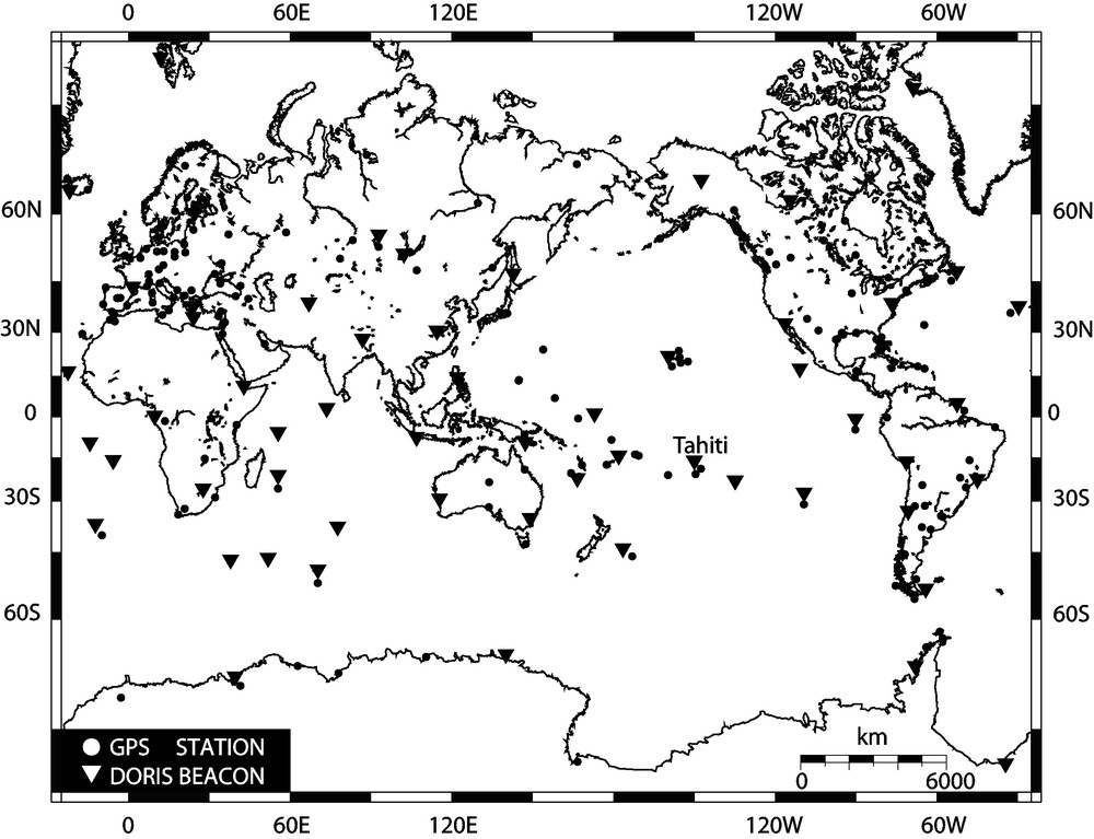
Geographical locations of the GPS stations involved in the GAMIT-GLOBK processing. DORIS beacons are indicated by triangles. At the Observatoire Géodésique de Tahiti, two GPS stations (THTI and TAH1), and DORIS beacon (PAUB) are co-located. At the Papeete port, PAPE GPS station and tide gauge are also co-located. In the NW Coast of Tahiti, FAA1 GPS station is maintained by Météo-France weather service. Neither FAA1 nor PAPE are included in the MIT reprocessed products.
Situations géographiques des stations GPS traitées à l’aide du logiciel GAMIT-GLOBK. Les balises DORIS sont indiquées par des triangles. Deux stations GPS (THTI et TAH1) et une balise DORIS (PAUB) sont co-localisées à l’Observatoire Géodésique de Tahiti. La station GPS (PAPE) et un marégraphe sont aussi co-localisés dans le port de Papeete. Située sur le littoral nord-ouest de Tahiti, la station GPS (FAA1) est maintenue par Météo France. Ni les observations de FAA1, ni celles de PAPE ne sont incluses dans les produits retraités de MIT.

This article aims to search for reconciling the coral reef stratigraphy estimates and the present study of the present-day vertical land motion of the Tahiti Island using GPS, DORIS, satellite altimetry, and tide gauge observations. The crustal uplift or subsidence rate is an important component not only for absolute sea level reconstruction but one needs it to account for in landscape evolution modeling, in particular, it must be included in the mass balance relationship. Such estimates may also provide new constraints for studies of the mechanical behavior of the oceanic lithosphere that deforms in response to surface loads.

With the significant improvements in GPS, DORIS, Satellite Laser Ranging (SLR), and Very Long Baseline Interferometry (VLBI) global networks and data analysis (e.g., Collilieux et al., 2007; King et al., 2008; Willis et al., 2009), height time series of geodetic stations are used extensively to: (1) investigate many geophysical processes such as local crustal deformation, sea-level changes, and glacial isostatic adjustment (GIA); (2) to validate and improve atmospheric, oceanic, and hydrological loading models; and (3) to strengthen the terrestrial reference frame representation.

More recently, on a regional and global scale, GPS and DORIS have achieved a level of maturity suitable for the comparison of high-precision vertical velocity fields to independent vertical rates derived from TG's only (Bouin and Wöppelmann, 2010), and from combined altimetry and TG data (e.g., Cazenave et al., 1999; Kuo et al., 2004; Ray et al., 2010). In a few cases, vertical DORIS and GPS results were also compared to postglacial models (e.g., Amalvict et al., 2009; Kierulf et al., 2009; King et al., 2010).

The OGT (Observatoire Géodésique de Tahiti) is one of the few geodetic observatories continuously operating three co-located space geodetic techniques: two GPS stations (THTI and TAH1), a DORIS beacon (PAUB), and an SLR system (THTL). We take advantage of the availability of 12 years of GPS and DORIS observations, 17 years of satellite altimetry data, and 35 years of TG sea level records to monitor the vertical displacement of the Tahiti Island using different software packages. Furthermore, direct comparison with independent source measurements based on coral reef stratigraphy (e.g., Bard et al., 1996, Pirazzoli and Montaggioni, 1988), and GIA models (e.g., Peltier, 2004) is also of great importance. We should, however, mention that a single measure of absolute gravimetry was made at the OGT observatory in June 2003 by the École et Observatoire des Sciences de la Terre (EOST) of Strasbourg (France).

Although, SLR is the most appropriate, among the space geodetic techniques, to accurately determine the vertical component (Degnan, 1993), the THTL time series have unfortunately undergone many gaps due to hardware failures and weather conditions, and thus are deemed insufficient in this study as this large number of breaks would create some significant uncertainties in the derived velocity, depending on the type of noise involved (Williams et al., 2004).

The satellite geodesy data used and their processing strategies are first described. The results are then presented and discussed.

2 Data sets and analysis

2.1 GPS vertical motion estimation approaches

The GPS data come from the International GNSS Service (IGS) stations (Dow et al., 2009), including Tahiti IGS stations (Fig. 1), and cover the time span from the beginning of 1998 to the end of 2009. Two strategies and software packages are used to process the GPS data. In the first strategy, an analysis of GPS phase data from over 300 stations is performed by MIT analysis center using GAMIT-GLOBK software (Herring et al., 2009; King and Bock, 2006) in a two-step network approach (Dong et al., 1998), and in a consistent way all over the considered data span.

In the first step, GPS phase observations are used from each day to estimate station coordinates, tropospheric zenith delays, horizontal gradients, and orbital and Earth Orientation Parameters (EOPs). Those daily products are submitted for ITRF2008 (Altamimi et al., 2011), and made publicly available at (ftp://everest.mit.edu/pub/MIT_GLL/).

In the second step, we use the loosely constrained estimates of station coordinates, orbits, and EOPs and their covariance matrix from each day, as quasi-observations in a Kalman filter to estimate a consistent set of coordinates and velocities.

To account for time-correlated sources of error in the station position estimates, including monument instability and signatures in the time series that may be due to errors in modeling the orbits or atmosphere, we calculate a unique noise model for each station. The algorithm used to model the data noise spectrum assumes that each time series can be adequately modeled using a First-Order Gauss Markov (FOGM) process noise described in the following equation (Gelb, 1974):

φ_{x x} (τ) = σ^{2} e^{- β | τ |}

where φ_xx(τ) is the FOGM autocorrelation function, σ² is the long-term variance, and β⁻¹ is the correlation time. Since GLOBK uses a random walk (RW) process noise model (which is a special case of the FOGM model where the correlation time β⁻¹ is infinite, we estimate a RW process noise model for each station from its time series (Fig. 2) by averaging the residuals over increasingly longer intervals (Herring et al., 2009). These RW process noise values are then used in the forward run of the GLOBK Kalman filter (using the same data set used in the time series) to estimate site velocities and realistic uncertainties.

Fig. 2
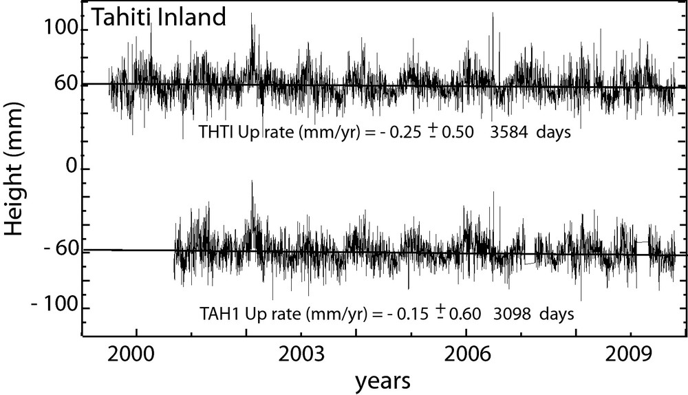
Height time series of THTI and TAH1 GPS stations derived from 07-HPT GAMIT-GLOBK daily solutions with respect to ITRF2005 reference frame. The time series are conventionally offset by 120 mm for clarity. The Linear trends and uncertainties are estimated with respect to white + flicker noise error models using CATS software (Williams, 2008).
Séries temporelles de la composante verticale des stations GPS (THTI et TAH1) résultant des solutions 07-HPT journalières de GAMIT-GLOBK, suivant le repère de référence ITRF2005. Les séries temporelles sont arbitrairement décalées de 120 mm pour mieux distinguer les profils. La tendance linéaire et les incertitudes sont estimées selon le modèle de bruit blanc + scintillation en utilisant le logiciel CATS (Williams, 2008).

The terrestrial reference frame of our 14-HPT velocity estimates is defined in the second step, in which generalized constraints are applied (Dong et al., 1998) while estimating Helmert's parameter transformations (HPT: three translations, three rotations, and scale factor and their rates of change) between our loosely constrained GPS analysis and the known ITRF2005 (Altamimi et al., 2007a) positions and velocities of 60 IGS stations. The obtained vertical GPS velocities with associated uncertainties are provided in the appendix in the electronic supplement (Appendix A).

In Fig. 3, we compare the GLOBK daily solutions (07-HPT) and the GLOBK weekly combined solution (14-HPT) shown in Appendix A. The mean difference between the two solutions is 0.09 ± 0.45 mm/yr. Although more than 97% of the 07-HPT vertical velocities agree with the 14-HPT vertical velocities within ± 1.0 mm/yr, there are a few stations for which the difference between the two solutions exceeds 1 mm/yr (e.g., GOUG, QAQ1, TSKB, USUD. [Appendix A]). This discrepancy may be due to, but not limited to the reference frame scale factor and its associated rate estimation.

Fig. 3
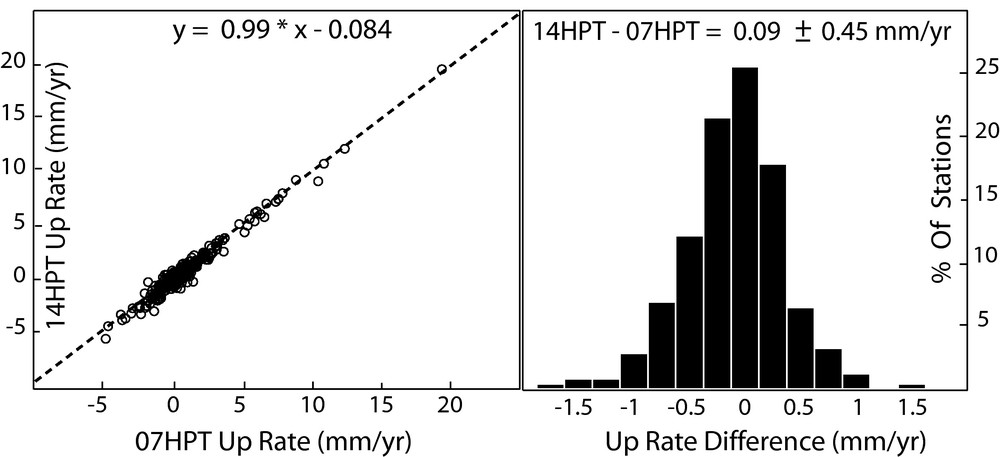
Comparison between the 07-HPT and 14-HPT height rate solutions by a linear fit and a histogram of the velocity difference (see Appendix A).
Comparaison entre les solutions de déplacement vertical 07-HPT et 14-HPT par ajustement linéaire et histogramme des différences de vitesse (voir Appendix A).

In the second strategy, only GPS data from FAA1, PAPE, TAH1, and THTI are processed with respect to the Precise Point Positioning (PPP) mode (Zumberge et al., 1997) of GIPSY-OASIS II (Webb and Zumberge, 1995) using JPL reprocessed products (ftp://sideshow.jpl.nasa.gov/pub/JPL_GPS_Products/Final/). We estimate station positions and clocks, phase biases, and tropospheric delays and horizontal tropospheric gradients. The a priori zenith hydrostatic delay (ZHD) is calculated based on the station height and thus regarded as constant, while the zenith wet delay (ZWD) and the horizontal tropospheric gradients (north G_N and east G_E) are modeled as Random Walk (RW) variables with variance of 3 $cm / \sqrt{h}$ for ZWD and 0.3 $cm / \sqrt{h}$ for G_N and G_E, and are estimated every 5 min as time-dependent parameters (Bar-Sever et al., 1998). The resulting daily solutions are aligned to the ITRF2005 reference frame using Helmert's parameter transformations (JPL x-files) (Table 1).

	GIPSY-OASIS II PPP MODE
Site	07-HPT Hgt Rate (mm/yr)	Data Span (yrs)
FAA1	−0.60 ± 1.60	4.02
PAPE	−0.40 ± 0.80	6.85
TAH1	−0.40 ± 0.60	9.70
THTI	−0.25 ± 0.50	10.85

The estimated site positions are projected in the local north, east and up components (Fig. 4) (usually this reference frame is referred as the NEU frame), cleaned to remove outliers using TSVIEW software (Herring, 2003), and analyzed using CATS software (Williams, 2008) for their noise properties, linear velocities, and periodic signals.

Fig. 4
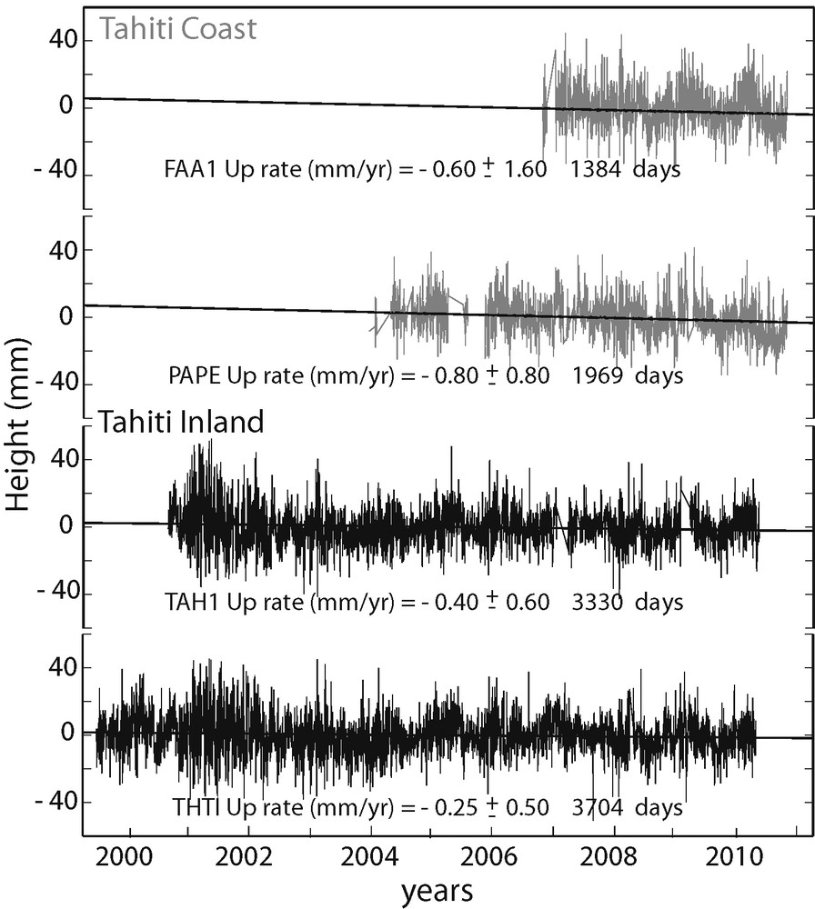
Height time series of FAA1, PAPE, TAH1 and THTI GPS stations derived from GIPSY-OASIS II PPP daily solutions with respect to ITRF2005 reference frame. The Linear trends and uncertainties are estimated using white + flicker noise error models (see text).
Séries temporelles de la composante verticale des stations GPS (FAA1, PAPE, TAH1 et THT1) résultant des solutions journalières de GIPSY-OASIS II PPP suivant le repère de référence ITRF2005. Les tendances linéaires et les incertitudes sont estimées selon le modèle de bruit blanc+ scintillation (voir texte).

It is now well known that the measurement noise associated with GPS positions is time correlated (e.g., Langbein and Johnson, 1997; Mao et al., 1999; Williams, 2003). In addition to white noise, the main process affecting GPS position time-series is almost a flicker noise (Amiri-Simkooei et al., 2007). Therefore, the model parameters (linear terms, annual and semi-annual periodic signals, and their associated uncertainties) are estimated using a white + flicker noise error models (Table 1).

Solid Earth and pole tide corrections following the IERS Conventions 2003 (McCarthy and Petit, 2004), ocean loading corrections using the FES2004 ocean tide model (Lyard et al., 2006), antenna phase center models (Schmid et al., 2007), and the Global Mapping Function (GMF) (Boehm et al., 2006) are taken into account in both software packages.

2.2 DORIS vertical motion estimation approach

DORIS is a French tracking system originally designed for precise orbitography of altimeter satellites (e.g., Willis et al., 2006). It is an uplink Doppler system with a dense and homogeneous tracking network (Fig. 1), allowing almost continuous observation for Low Earth Orbiting (LEO) satellites. It quickly became very useful for high-precision geodesy, including determination of vertical crustal motions (e.g., Mangiarotti et al., 2001; Ray et al., 2010; Soudarin et al., 1999).

DORIS data over 1993–2009 on all available satellites (SPOT2, SPOT3, SPOT4, SPOT5, TOPEX-Poseidon, Envisat) are processed by the IGN group in a free-network approach using the GIPSY-OASIS II software (Willis et al., 2010a). Jason-1 data are not used in the current solution due to the problem related to the South Atlantic Anomaly (Lemoine and Capdeville, 2006; Willis et al., 2004). Daily stations positions and EOP are combined on a weekly basis, projected and transformed into the ITRF2005 reference frame using 07-HPT estimation strategy.

The DORIS beacon (PAPB), initially installed in 1995, has been moved by a few hundred meters in 1998 to the OGT observatory building (PAQB). It has been upgraded to a third generation one (PATB) on October, 3^rd, 2007 (Fagard, 2006). The Starec antenna, and supporting plate and tower were changed. On November, 18^th, 2009, the station became the fourth Master Beacon in the DORIS network (PAUB). While the name is different (PATB and PAUB), in such a case, the antenna and its reference point remain the same. The clock used to time tag the DORIS measurements is changed to a better frequency standard. The GPS station THTI is located a few meters away (DX = −1.119 m, DY = 6.358 m, DZ = −2.363 m). However, the GLOSS #140 tide gauge is located on the coast about 6 km away (DX = 623.406 m, DY = −3,773.553 m, DZ = 4,636.646 m). GLOSS stands Global sea level observing system and is a worldwide programme for tide gauge observations (Woodworth et al., 2009).

Weekly station position time series were used for PAQB and PATB DORIS stations (Fig. 5). These solutions are derived from the latest IGN/JPL solutions known as ignwd09 (Willis et al., 2010a) and made available at the International DORIS Service (IDS) (Tavernier et al., 2002; Willis et al., 2010b) (ftp://doris.ign.fr/pub/doris/products/sinex_series/ignwd) and (ftp://cddis.gsfc.nasa.gov/pub/doris/products/sinex_series/ignwd). We do not consider PAPB located a few hundred meters from the OGT observatory since there may have local effects, and PAUB because it had too little data available at the time of this study (some months more that do not change the slope itself, but need to introduce a potential bias change of equipment). So it will be useful in the future.

Fig. 5
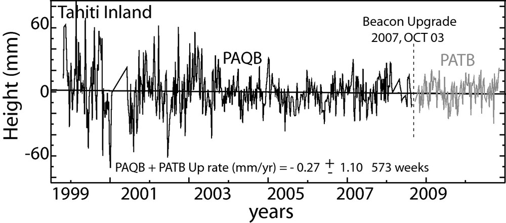
Height time series of (PAQB + PATB) DORIS beacon derived from ignwd09 IGN/JPL weekly solutions with respect to the ITRF2005 reference frame. The Up rate indicates the linear trend. Antenna change on October, 3^rd, 2007 (dashed line) presented an offset of (10.04 ± 2.30) mm in the considered time series.
Série temporelle de la composante verticale de la balise DORIS (PAQB + PATB) résultant des solutions hebdomadaires ignwd09 de l’IGN/JPL, suivant le repère de référence ITRF2005. « Up rate » indique la tendance linéaire. Le changement d’antenne (3 octobre 2007, en ligne pointillée) a créé un saut de 10,04 ± 2,30 mm dans la série temporelle considérée.

The ignwd09 solution strengths are essentially related to the new models used and the analysis strategy adopted for the whole processing period. Strictly speaking, improvements come from the new gravity field model GGM03S (Tapley et al., 2005), the solar radiation pressure fixing (Gobinddass et al., 2009a,b), the hourly atmospheric drag parameter estimation (Gobinddass et al., 2010), the tropospheric Global Mapping Function (GMF) (Boehm et al., 2006), and the 10° degrees elevation cut-off angle.

2.3 Vertical land motion from altimetry data and tide gauge records

The Tide gauges (TG) constrain the relative sea level (RSL) change, which is the variation in the position of the sea surface relative to the solid earth. Given the absolute (geocentric) sea level rate (ASL) (i.e. with respect to the earth's center of mass within a well-defined terrestrial reference frame), it might be possible to estimate the vertical motion ${\dot{H}}_{T G}$ of the benchmarks to which TG's are referenced, and then ${\dot{H}}_{T G}$ can be written as:

{\dot{H}}_{T G} = A S L - R S L

The RSL trend is estimated from Papeete TG data. Used here are monthly mean sea levels from the archive of the University of Hawaii Sea Level Center (UHSLC) from July 1975 through December 2009 (Fig. 6), a seven years extension of the Revised Local Reference (RLR) data set of the Permanent Service for Mean Sea Level (PSMSL) (Woodworth and Player, 2003). Both UHSLC and PSMSL records are checked and corrected for local datum changes.

Fig. 6
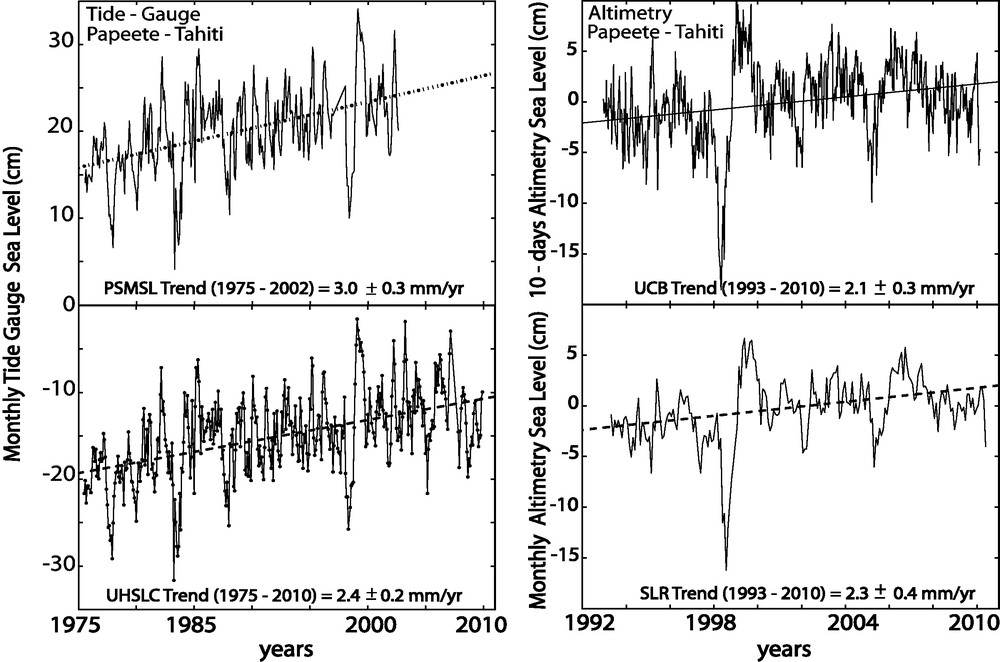
Left: Monthly Papeete (Tahiti) tide gauge sea level time series computed by PSMSL for the period (1975–2002), and recently by UHSLC for the period (1975–2010). Time series are shifted for clarity. Right: Sea level time series extracted from near-global gridded arrays of altimetric data every 10 days from UCB (http://sealevel.colorado.edu), and monthly from CSIRO (SLR) (http://www.cmar.csiro.au/sealevel/). The standard errors associated with the trends are derived from the time series using a white noise model only using CATS software (Williams, 2008). The El Niño events (1982–1983 and 1998–1999) are clearly apparent in the time series.
À gauche : Séries temporelles mensuelles du niveau de la mer du marégraphe de Papeete (Tahiti), calculées par PSMSL pour la période 1975–2002, et plus récemment par UHSLC pour la période (1975–2010). Les séries temporelles sont arbitrairement décalées pour mieux distinguer les profils. À droite : Séries temporelles du niveau de la mer extraites des grilles globales d’altimétrie, avec un pas de temps de 10 jours provenant de UCB, (http://sealevel.colorado.edu), et avec un pas de temps mensuel de CSIRO (SLR) (http://www.cmar.csiro.au/sealevel/). Les incertitudes associées aux tendances linéaires sont calculées d’après un modèle de bruit blanc en utilisant le logiciel CATS (Williams, 2008). Les événements El Niño (1982–1983 et 1998–1999) apparaissent nettement dans les séries temporelles.

The ASL trend can be regarded as the mean value of the absolute 20th century global sea level (AGSL) which is estimated from a large number of a globally well-distributed TG's with complete long term records and corrected for vertical land motion using the most recent GIA models (e.g., Peltier, 2004). Following this approach, Bindoff et al. (2007) found an AGSL value of 1.8 ± 0.5 mm/yr for the period 1961–2003, which is consistent with previous estimated rates (Church and White (2006), 1.7 ± 0.3 mm/yr, and Douglas (2001), 1.8 ± 0.5 mm/yr). Bouin and Wöppelmann (2010) supposed that the difference between the RSL trend measured by an individual TG and the global mean value AGSL is mainly due to the TG vertical motion and not to local ASL variations that are significantly different from 1.8 ± 0.5 mm/yr.

The ASL trend can be also derived from satellite altimetry measurements. In fact, the University of Colorado at Boulder (UCB) Sea Level Change (Leuliette et al., 2004) and the Australian CSIRO Sea Level Rise (SLR) provide 10 days and monthly near-global gridded arrays of altimetric time series respectively. Time series are computed from TOPEX/Poseidon (T/P), Jason-1, and Jason-2, which have monitored the same ground track since 1992. In average, the vertical velocity of Papeete TG is −0.2 ± 0.2 mm/yr relative to the ASL trends computed from The CSIRO and UCB altimetry time series (Table 2).

Table 2

Comparaison entre déplacements verticaux du marégraphe de Papeete ( ${\dot{H}}_{T G}$ ), obtenus dans notre étude et ceux issus d’autres travaux. WT-IB et WO-IB représentent l’effet du Baromètre Inverse. La correction IB n’est pas appliquée au marégraphe de Papeete, puisque Ponte (2006) a montré que ce signal était négligeable (d’environ 0,1 mm/an pour les séries temporelles de l’altimétrie de CSIRO), mais il est important de la prendre en considération dans le cas de Papeete. L’incertitude de ${\dot{H}}_{T G}$ est associée à la série temporelle de RSL.

ASL (mm/yr)	ASL Ref.	RSL (mm/yr)	RSL Ref.	RSL Data Span	${\dot{H}}_{T G}$ (mm/yr)	Source
2.3 ± 0.4	CSIRO (SLR) WT-IB	2.4 ± 0.2	UHSLC	1975–2010	−0.1 ± 0.2	This Study
2.2 ± 0.4	CSIRO (SLR) WO-IB	2.4 ± 0.2	UHSLC	1975–2010	−0.2 ± 0.2	This Study
2.1 ± 0.3	UCB WT-IB	2.4 ± 0.2	UHSLC	1975–2010	−0.3 ± 0.2	This Study
1.8 ± 0.5	Bindoff et al. (2007)	3.0 ± 0.3	PSMSL	1975–2002	−1.2 ± 0.3	Bouin and Wöppelmann (2010)
1.7 ± 0.3	Church and White (2006)	1.8 ± 0.5	Church et al. (2006)	1950–2002	−0.1 ± 0.5	This Study
1.8 ± 0.5	Ray et al. (2010)	2.5 ± 0.5	Ray et al. (2010)	1995–2009	−0.7 ± 0.5	Ray et al. (2010)

The ASL and RSL trends can also be taken from a reconstruction of global mean sea level using TG's sea level time series. Church and White (2006) made a reconstruction back to 1870 and found a sea level rise from January 1870 to December 2004 of 195 mm, and a 20th century ASL trend of 1.7 ± 0.3 mm/yr. Church et al. (2006), on shorter global sea level reconstruction (52 years), reported that an RSL of Papeete TG is to be at the level of 1.8 ± 0.5 mm/yr, which yields a subsidence rate consistent with CSIRO and UCB data (Table 2).

To compute the vertical land motion, Ray et al. (2010) followed the approach developed by Mitchum (1998) to monitor the stability of satellite altimeters with TG's. It consisted of differencing the TG sea level time series with an equivalent from satellite altimetry, while assuming that the difference will be dominated by vertical land motion at the TG benchmark, provided that both instruments measure an identical ocean signal (Fig. 7). Based on this approach, the height rate of Papeete TG is −0.7 ± 0.5 mm/yr which is, within one sigma uncertainty, consistent with rates derived from CSIRO and UCB data, but we note however that Ray et al. (2010) ASL trend is slightly lower than CSIRO and UCB, thing that may be due to, but not limited to intersatellite calibration biases (e.g., Leuliette et al., 2004). Indeed, if we consider only the T/P satellite, the vertical land motion of Papeete TG is in the order of −0.2 ± 0.9 mm/yr (Fig. 7).

Fig. 7
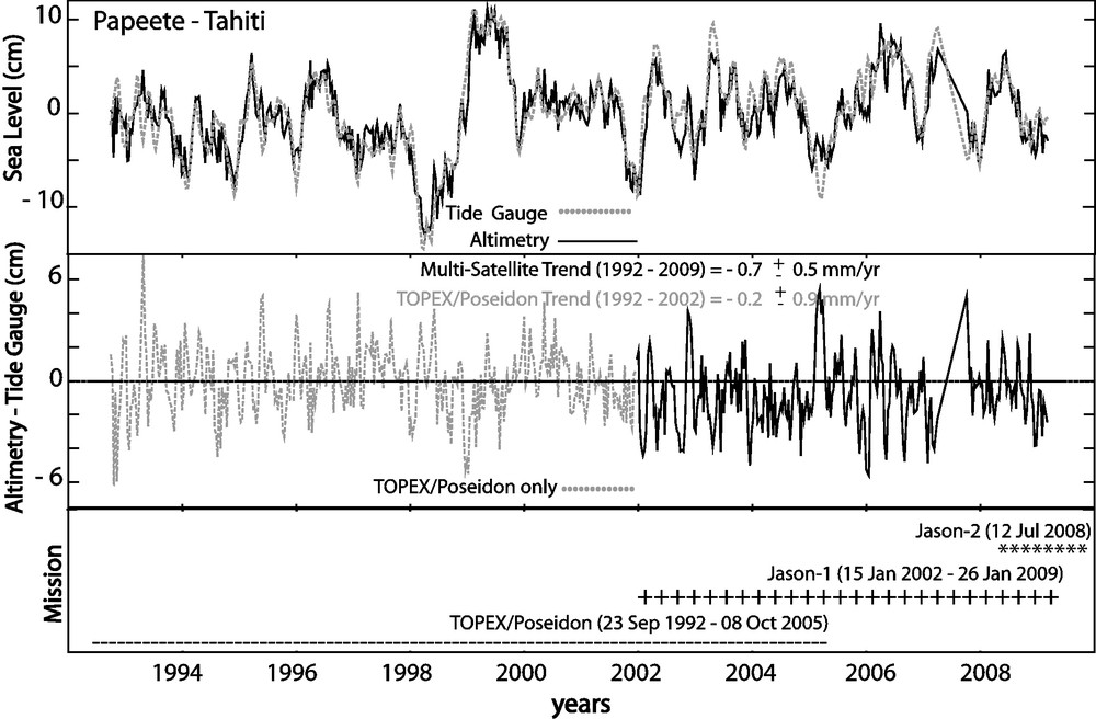
(Top) Altimetric and tide gauge sea level at Papeete, Tahiti island. (Middle) Difference between altimetric and tide gauge sea level time series, each point representing 10-day estimate. Multi-satellite trend is for the entire time series, while TOPEX/Poseidon trend ends at the Jason-1 first cycle (15 Jan 2002). (Bottom) Satellite mission start and end dates.
(En haut) : Séries temporelles du niveau de la mer de Papeete (Tahiti), à partir de l’altimétrie et du marégraphe. (Au milieu) : Différence entre ces deux séries temporelles, avec un intervalle de temps de 10 jours. La tendance « multi-satellites » représente la série temporelle complète, tandis que celle de TOPEX/Poséidon se termine au premier cycle de Jason-1 (15 janvier 2002). (En bas) : Début et fin des missions des satellites.

All Papeete TG vertical rates reported in Table 2 are consistent except the vertical rate that came from Bouin and Wöppelmann (2010). The main cause for this discrepancy is due to the difference between the UHSLC and PSMSL RSL's (which is about −0.6 mm/yr).

3 Vertical motion rates comparison

The estimated vertical rates based on GPS, DORIS, Satellite altimetry, tide gauge, coral stratigraphy, and GIA are shown in Table 3.

Table 3

Déplacements verticaux estimés à partir de GPS, de DORIS, du niveau de la mer, de la stratigraphie et de GIA. GG et GOA se réfèrent aux logiciels GAMIT-GLOBK et GIPSY-OASIS II. La vitesse de subsidence −0,5 mm/an est la moyenne des vitesses verticales des stations TAH1, THTI, PAPE et FAA1. CATREF est le logiciel développé par le centre d’analyse IGN (Altamimi et al., 2007b). Dist. représente la distance entre la technique de mesure donnée et le marégraphe de Papeete.

Data		Hgt Rate (mm/yr)	Dist. (km)
GPS	THTI: GG and GOA	−0.25 ± 0.50	6
GPS	TAH1: GG and GOA	−0.30 ± 0.60	6
GPS	THTI: CATREF/ITRF2008	−0.04 ± 0.20	6
GPS	FAA1: GOA	−0.60 ± 1.60	5
GPS	PAPE: GOA	−0.80 ± 0.80	0
DORIS	PAQB + PATB: GOA	−0.27 ± 1.10	6
TG Sea level	Papeete: GLOSS #140	−0.20 ± 0.30	0
Stratigraphy	Pirazzoli and Montaggioni (1988)	−0.15	2
Stratigraphy	Bard et al. (1996)	−0.25	2
GIA	Peltier (2004): ICE-5G (VM2 L90)	+0.17	–

Vertical velocities for Tahiti inland GPS stations (THTI and TAH1) are similar following the 14-HPT and 07-HPT estimation algorithm, with respect to GAMIT-GLOBK and GIPSY-OASIS II softwares (Appendix A and Table 1). Coastal GPS stations (FAA1 and PAPE) show slightly greater vertical land motion values than the inland ones (Table 1), but this could be explained by the nature of the land where the GPS stations were deployed: the site of FAA1 was an ancient ‘motu’ called Tahiri, a tiny sandy-coral island, before the International Airport of Faa’a was built in the 1960s whereas the PAPE station was co-located on the tide gauge pier so directly above the lagoon. Of course, differential movements exist within a volcano, and here, this could be due to local instable type of land. However, we believe the overall submillimeter rate, an order of magnitude found in previous geological studies for several inactive oceanic volcanoes in postshield stage, here obtained by the GPS estimates, is a precious indication of the vertical motion of the inner and coastal parts of the Island of Tahiti.

We also attempt to compare the 07-HPT GLOBK height rates with the ITRF2008, which includes DORIS, SLR, and VLBI techniques (Fig. 8). The number of common sites is 206. More than 95% of the 07-HPT vertical velocities agree with the ITRF2008 within ± 1.5 mm/yr, which confirm the consistency between the 07-HPT and the ITRF2008 vertical velocity fields.

Fig. 8
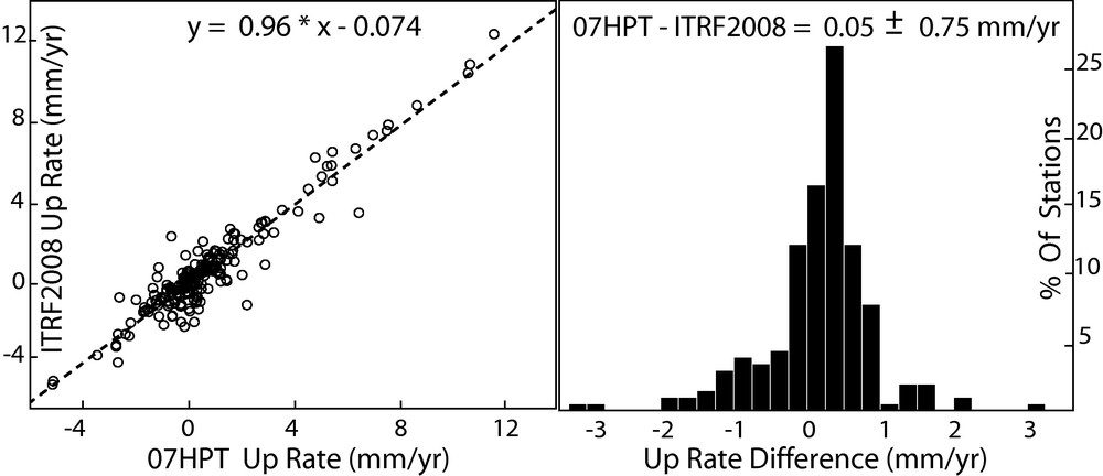
Comparison between the first release of the ITRF2008 vertical rate and the 07-HPT height rate solution. The linear trend and the histogram of the velocity difference are based on 206 GPS stations.
Comparaison entre les vitesses verticales de la première version de l’ITRF2008 et de la solution 07-HPT. Le calcul de la tendance linéaire et de l’histogramme des différences de vitesse prend en compte 206 stations GPS.

In particular, THTI is almost fixed following the ITRF2008 (Table 3), which is understood if we know already that present-day uncertainty in the ITRF reference frame scale factor is to be of order 0.1 ppb/yr, which translates to about 0.6 mm/yr in the vertical.

It must be noted that the DORIS vertical rate is in excellent agreement with the GPS-derived rate, while no attempt was done to due the DORIS terrestrial reference frame toward the GPS terrestrial reference frame, except to express both results independently into ITRF2005. Furthermore, recent vertical DORIS rates were provided for high-latitude tracking stations in Norway (Kierulf et al., 2009) and in Antarctica (Amalvict et al., 2009), for which more DORIS data are available due to the accumulation of satellite tracks of almost polar orbits (SPOTs and Envisat). For Tahiti, less data are available due to its latitude, and DORIS data are less numerous than for high-latitude stations. Vertical results may then be more difficult to obtain in Tahiti. Finally, the specific of the Tahiti station in a tropical area does not seem to degrade the derived vertical velocity. This probably comes from the way the tropospheric parameters were estimated in the GPS and DORIS data processing.

Moreover, Tahiti GPS subsidence is also very consistent with vertical motion derived from other measurements that are independent to reference frame scale factor, mainly the stratigraphy and the TG sea level. Vertical rates obtained from Tahiti corals sea-level records are not below −0.44 mm/yr and do not exceed −0.15 mm/yr (Bard et al., 1996, Cabioch et al., 1999; Camoin et al., 2007, Montaggioni et al., 1997; Pirazzoli and Montaggioni, 1988) (Table 3). Papeete TG vertical land motion supports this within one sigma uncertainty.

The predicted present-day radial motion of + 0.17 mm/yr from the ICE-5G (VM2 L90) PostGlacial Rebound model represents a slow uplift for the study area corresponding to the ‘far-field’ component of the solid Earth deformation in response to ice sheets mass redistribution causing changes in sea level (i.e. surface ocean loading). Consequently, any redistribution of mass on or within the Earth will perturb the geopotential and thus affect the ocean surface. Our GPS vertical motion rates (mean value of four estimates is −0.5 mm/yr, see Table 3) may reflect the sum of local effect (land compaction), effects of volcano loading and eventually neighbour loads and thermal plate contraction plus the GIA component.

We also need to point out that the implicit terrestrial reference frame used for geophysical models, such as GIA, may not be rigorously the same of the various ITRFs (Argus et al., 2010). However, as the large geocenter drifts are usually observed in the Z component, this frame difference will not affect the vertical velocity of this specific location in French Polynesia. However, for plate motion discussion, such imprecision in terrestrial reference frames should be taken into account.

4 Discussion and conclusion

Given such a low subsidence rate, there remains at least one important signal to investigate carefully in the future. In fact, space geodetic applications necessitate to model the tropospheric delays (related to atmospheric water vapor content or refractivity) as good as possible to obtain highly accurate positioning estimates. The models commonly used in the existing orbitography software packages cannot help to reconstruct complex refractivity fields which are likely to occur during extreme weather events such as storms and intense precipitations, in particular in the tropical Tahiti Island. Indeed, Hobiger et al. (2009) showed significant improvement in terms of GPS station height repeatabilities using a fine-mesh numerical weather model. In addition, the long-term atmospheric contribution can have a significant impact on the estimated linear trends of the vertical component. Nilsson and Elgered (2008) reported, for numerous GPS sites in Finland and Sweden, linear trends of zenith wet delays for 10-year periods reaching annual submillimetric rates in absolute values. As pointed out by Trenberth et al. (2003), these trends also tend to be higher in the Pacific Ocean than in Europe.

The above overall estimates of vertical land motion for Tahiti (mean value of −0.5 mm/yr, see Table 3) provide solid evidence on the present low subsidence rate which turns to be consistent with the rates independently derived from geological and coral reef records (Bard et al., 1996, Leroy, 1994, Montaggioni et al., 1997; Pirazzoli and Montaggioni, 1988). Note that the coral reef records concern the Last Glacial Maximum and Holocene reefs. To discuss the reliability of such estimate, we comment the results obtained for the Hawaiian GPS sites. This is justified by the similar geological settings characterizing Big Island-Kauai and Mehetia-Maupiti Islands sequences, given the age of the oceanic lithosphere at the time of volcanic loading and the 0 to 4-6 Ma hotspot tracks, while the two volcanic alignments have differences in terms of dimension, spatial distribution or volcanic formation rate. First the HILO, MKEA and UPO1 sites located in the Big Island (Appendix A), a large active volcano, exhibit well similar relatively high subsidence rates (−2.5 to −1.5 mm/yr) presented in previous work by Caccamise et al. (2005) using GPS data as well as geological study by Moore (1987); second, the other Hawaiian stations located in inactive volcanoes (HLNC, LHUE, KOK1), except the KOKB and MAUI sites, show clear submillimeter rates. The interesting point is that the postshield erosional Hawaiian Islands and Tahiti which ages are greater than 1.5 Ma old are rather subsiding at submillimeter rate. Instead, Caccamise et al.’s (2005) estimates from short 6-year time span gave millimeter rates probably less reliable than ours. Considering the volcanic evolution of oceanic islands, the construction is often completed in less than 1–3 Myr for the Hawaiian and Tahitian Islands (this can be greater than 12 Myr as for the Canarian Islands (e.g., Carracedo, 1999). There are three phases, the shield-stage that builds up the bulk of the volcano structure during a few of hundred thousands of years accompanied eventually by huge landslides, the transition called the postshield capping stage and the posterosional stage. The differential subsidence rate is somehow related to the evolutionary stages but possibly modulated by plume-plate interaction and/or flexural lithospheric deformation caused by surrounding loads (Watts and ten Brink, 1989; Watts and Zhong, 2000; Wessel and Keating, 1994; Zhong and Watts, 2002) and erosional mass redistributions, the thermal cooling contribution being negligible for relatively old plates. Finally, the estimates of magnitudes of the vertical motion are in good agreement with the conclusions of the recent studies on the history of the subsidence of the Maui-Nui Complex (Maui, Molokai, Lanai and Kahoolawe) and Hawaii Island, based on submerged terraces that are mostly drowned reefs developed over the past 2 Ma (Faichney, 2010; Faichney et al., 2010). Faichney (2010) estimated the initial subsidence rates around 1 mm/yr for the Maui-Nui Complex but also supported that the Maui-Nui complex (since the initial stage) slowly subsides as the lithosphere flexes in response to the volcanic loading of the complex itself and the Big Island of Hawaii.

Acknowledgments

We thank CalTech/JPL for providing the GIPSY-OASIS II and MIT/EAPS for GAMIT-GLOBK. Figures were produced using Generic Mapping Tools (Wessel and Smith, 1995). We also thank the IGS and IDS centers for GPS and DORIS products Noll (2010). Satellite altimetry time series were obtained from CSIRO (SLR) and UCB, as well as Tide Gauge data from PSMSL and UHSL Sea level difference (Altimetry - TG) computed by Richard D. Ray from NASA GSFC (Ray et al., 2010). We are grateful to anonymous reviewers for their careful and constructive reviews. This work was supported by the Agence Nationale de la Recherche (ANR Contrat État Polynésie Française 2006) and the Centre National d’Études Spatiales (CNES DAR OGT 2008). Part of this work is based on observations from the DORIS system. This paper is IPGP contribution number 3107.

References

[Altamimi et al., 2007a] Altamimi, Z., Collilieux, X., Legrand, J., Garayt, B., Boucher, C., 2007a. ITRF2005: a new release of the International Terrestrial Reference Frame based on time series of station positions and Earth Orientation Parameters. J. Geophys. Res., 112, B09401, doi:10.1029/2007JB004949.

[Altamimi et al., 2007b] Altamimi, Z., Sillard, P., Boucher, C., 2007b. CATREF software: Combination and Analysis of Terrestrial Reference Frames. Release and Documentation of May 2007, Institut Géographique National, Paris, France.

[Altamimi et al., 2011] Altamimi, Z., Collilieux, X., Métivier, L., 2011. ITRF2008: an improved solution of the international terrestrial reference frame. J. Geod., 85 (5), . | DOI

[Amalvict et al., 2009] M. Amalvict; P. Willis; G. Wöppelmann; E.R. Ivins; M.N. Bouin; L. Testud; J. Hinderer Stability of the East Antarctic station Dumont d’Urville from long-term geodetic and geophysical observations, Polar Res., Volume 28 (2009) no. 2, pp. 193-202

[Amiri-Simkooei et al., 2007] Amiri-Simkooei, A.R., Tiberius, C.C.J.M., Teunissen, P.J.G., 2007. Assessment of noise in GPS coordinate time series: methodology and results. J. Geophys. Res., 112, B07413, doi:10.1029/2006JB004913.

[Argus et al., 2010] D.F. Argus; R.G. Gordon; M.B. Helin; C. Ma; R. Eanes; P. Willis; W.R. Peltier; S. Owen The angular velocities of the plates and the velocity of the Earth's center from space geodesy, Geophys. J. Int., Volume 180 (2010) no. 3, pp. 916-960

[Bar-Sever et al., 1998] Y.E. Bar-Sever; P.M. Kroger; J.A. Borjesson Estimating horizontal gradients of tropospheric path delay with a single GPS receiver, J. Geophys. Res., Volume 103 (1998) no. B3, pp. 5019-5035

[Bard et al., 1996] E. Bard; B. Hamelin; L. Montaggioni; G. Cabioch; G. Faure; F. Rougerie Deglacial sea-level record from Tahiti corals and the timing of global meltwater discharge, Nature, Volume 382 (1996), pp. 241-244

[Bindoff et al., 2007] N.L. Bindoff; J. Willebrand; V. Artale; A. Cazenave; J. Gregory; S. Gulev; K. Hanawa; C. LeQuere; S. Levitus; Y. Nojiri; C.K. Shum; L.D. Talley; A.S. Unnikrishnan Observations: oceanic climate change and sea level (S. Solomon; D. Qin; M. Manning; M. Marquis; K. Averyt; M.M.B. Tignor; H.L. Miller; Z. Chen, eds.), Climate change 2007: The physical science basis. Contribution of Working Group first to the fourth assessment report of the intergovernmental panel on climate change, Cambridge University Press, New York, 2007, pp. 385-432

[Boehm et al., 2006] Boehm, J., Niell, A.E., Tregoning, P., Schuh, H., 2006. The Global Mapping Function (GMF): A new empirical mapping function based on numerical weather model data. Geophys. Res. Lett., 33 (7), L07304.

[Bouin and Wöppelmann, 2010] M.N. Bouin; G. Wöppelmann Land motion estimates from GPS at tide gauges: a geophysical evaluation, Geophys. J. Int., Volume 180 (2010), pp. 193-209

[Cabioch et al., 1999] G. Cabioch; G. Camoin; L. Montaggioni Postglacial growth history of a French Polynesian barrier reef tract, central Pacific, Sedimentology, Volume 46 (1999), pp. 985-1000

[Caccamise et al., 2005] Caccamise, D.J., II, Merrifield, M.A., Bevis, M., Foster, J., Firing, Y.L., Schenewerk, M.S., Taylor, F.W., Thomas, D.A., 2005. Sea level rise at Honolulu and Hilo, Hawaii: GPS estimates of differential land motion. Geophys. Res. Lett., 32, L03607, doi:10.1029/2004GL021380.

[Camoin et al., 2007] G.F. Camoin; Y. Iryu; D.B. McInroy; and the IODP Expedition 310 Scientists IODP Expedition 310 reconstructs sea level, climatic, and environmental changes in the South Pacific during the last deglaciation, Sci. Drill., Volume 5 (2007), pp. 4-12

[Carracedo, 1999] J.C. Carracedo Growth, structure, instability and collapse of Canarian volcanoes and comparisons with Hawaiian volcanoes, J. Volcanol. Geotherm. Res., Volume 94 (1999), pp. 1-19

[Cazenave et al., 1999] Cazenave, A., Dominh, K., Ponchaut, F., Soudarin, L., Crétaux, J.F., Le Provost, C., 1999. Sea level changes from TOPEX-Poseidon altimetry and tide gauges, and vertical crustal motions from DORIS. Geophys. Res. Lett., 26(14), 2077-2080, doi:10.1029/1999GL900472.

[Church and White, 2006] Church, J.A., White, N.J., 2006. A 20th century acceleration in global sea level rise. Geophys. Res. Lett., 33, L01602, doi:10.1029/2005GL024826.

[Church et al., 2006] Church, J.A., White, N.J., Hunter, J.R., 2006. Sea level rise at tropical Pacific and Indian Ocean islands. Global and Planetary Change, 53, 155-168, doi:10.1016/j.glopacha.2006.04.001.

[Clouard et al., 2001] V. Clouard; A. Bonneville; P.Y. Gillot A giant landslide on the southern flank of Tahiti Island, French Polynesia. Geophys. Res. Lett., Volume 28 (2001), pp. 2253-2256

[Collilieux et al., 2007] Collilieux, X., Altamimi, Z., Coulot, D., Ray, J., Sillard, P., 2007. Comparison of very long baseline interferometry, GPS, and satellite laser ranging height residuals from ITRF2005 using spectral and correlation methods. J. Geophys. Res., 112, B12403, doi:10.1029/2007JB004933.

[Degnan, 1993] J. Degnan Millimeter accuracy Satellite Laser Ranging: a review (D. Smith; D. Turcotte, eds.), American Geophysical Union (AGU), Geodynamics Series Contributions of Space Geodesy to Geodynamics, 25, Crustal Dynamics, Washington, DC, 1993, pp. 733-762

[Dong et al., 1998] D. Dong; T.A. Herring; R.W. King Estimating regional deformation from a combination of space and terrestrial geodetic data, J. Geod., Volume 72 (1998), pp. 200-211

[Douglas, 2001] B.C. Douglas Sea level change in the era of the recording tide gauge (B.C. Douglas; M.S. Kearney; S.P. Leatherman, eds.), Sea Level Rise, Academic Press, San Diego, 2001, pp. 37-64

[Dow et al., 2009] J.M. Dow; R.E. Neilan; C. Rizos The International GNSS Service in a changing landscape of Global Navigation Satellite System, J. Geod., Volume 83 (2009) no. 3–4, pp. 191-198

[Fagard, 2006] Fagard, H., 2006. Twenty years of evolution for the DORIS permanent network: from its initial deployment to its renovation. J. Geod., 80 (8–11), 429-456, doi:10.1007/s00190-006r-r0084-2.

[Faichney, 2010] Faichney, I.D.E., 2010. The Geology of the submerged reefs in the Maui-Nui Complex, Hawaii. James Cook University, PhD thesis, 215 p.

[Faichney et al., 2010] Faichney, I.D.E., Webster, J.M., Clague, D.A., Paduan, J.B., Fullagar, P.D., 2010. Unraveling the tilting history of the submerged reefs surrounding Oahu and the Maui Nui Complex, Hawaii. Geochem. Geophys. Geosyst., 11, Q07002, doi:10.1029/2010GC003044.

[Gelb, 1974] A. Gelb Applied Optimal Estimation, MIT Press, Cambridge, Mass, 1974

[Gobinddass et al., 2009a] Gobinddass, M.L., Willis, P., de Viron, O., Sibthorpe, A., Zelensky, N.P., Ries, J.C., Ferland, R., Bar-Sever, Y.E., Diament, M., 2009a. Systematic biases in DORIS-derived geocenter time series related to solar radiation pressure mis-modeling. J. Geod., 83(9), 849-858, doi:10.1007/s00190-009r-r0303-8.

[Gobinddass et al., 2009b] Gobinddass, M.L., Willis, P., Sibthorpe, A.J., Zelensky, N.P., Lemoine, F.G., Ries, J.C., Ferland, R., Bar-Sever, Y.E., de Viron, O., Diament, M., 2009b. Improving DORIS geocenter time series using an empirical rescaling of solar radiation pressure models. Adv. Space Res., 44(11), 1279-1287, doi:10.1016/j.asr.2009.08.004.

[Gobinddass et al., 2010] Gobinddass, M.L., Willis, P., Menvielle, M., Diament, M., 2010. Refining DORIS atmospheric drag estimation in preparation of ITRF2008. Adv. Space Res., 46(12), 1566-1577, doi:10.1016/j.asr. 2010.04.004.

[Herring, 2003] T.A. Herring Matlab Tools for viewing GPS velocities and time series, GPS solutions, Volume 7 (2003) no. 3, pp. 194-199

[Herring et al., 2009] T.A. Herring; R.W. King; S. McClusky GLOBK: Global Kalman filter VLBI and GPS analysis program. Version 10.3, Massachusetts Institute of Technology, Cambridge, 2009

[Hildenbrand et al., 2008] A. Hildenbrand; P.Y. Gillot; C. Marlin Geomorphological study of long-term erosion on a tropical volcanic ocean island: Tahiti-Nui (French Polynesia), Geomorphology, Volume 93 (2008) no. 3–4, pp. 460-481

[Hobiger et al., 2009] T. Hobiger; S. Shimada; S. Shimizu; R. Ichikawa; Y. Koyama; T. Kondo Improving GPS positioning estimates during extreme weather situations by the help of fine-mesh numerical weather models, J. Atmos. Solar-Terrestrial Phys., Volume 72 (2009) no. 2–3, pp. 262-270 (Feb. 2010)

[Kierulf et al., 2009] H.P. Kierulf; B. Pettersen; D.S. McMillan; P. Willis The kinematics of Ny-Alesund from space geodetic data, J. Geodyn., Volume 48 (2009) no. 1, pp. 37-46

[King et al., 2008] King, M.A., Watson, C.S., Penna, N.T., Clarke, P., 2008. Subdaily signals in GPS observations and their effect at semiannual and annual periods. Geophys. Res. Lett., 35, L03302, doi:10.1029/2007GL032252.

[King et al., 2010] M.A. King; Z. Altamimi; J. Boehm; M. Bos; R. Dach; P. Elosegui; F. Fund; M. Hernandez-Pajares; D. Lavallee; P.J.M. Verveira; R.E.M. Riva; P. Steigenberger; T. van Dam; L. Vittuari; S.D.P. Williams; P. Willis Improved constraints on models of glacial isostatic adjustment, A review of the contribution of ground-based geodetic observations, Surv. Geophys., Volume 31 (2010) no. 5, pp. 465-507

[King and Bock, 2006] R.W. King; Y. Bock Documentation for GAMIT analysis software, release 10.3, Massachusetts Institute of Technology, Cambridge, 2006

[Kuo et al., 2004] Kuo, C.Y., Shum, C.K., Braun, A., Mitrovica, J.X., 2004. Vertical crustal motion determined by satellite altimetry and tide gauge data in Fennoscandia. Geophys. Res. Lett., 31, L01608, doi:10.1029/2003GL019106.

[Langbein and Johnson, 1997] J. Langbein; H. Johnson Correlated errors in geodetic time series: implications for time dependent deformation, J. Geophys. Res., Volume 102 (1997) no. B1, pp. 591-603

[Lemoine and Capdeville, 2006] Lemoine, J.M., Capdeville, H., 2006. A corrective model for Jason-1 DORIS Doppler data in relation to the South Atlantic Anomaly. J. Geod., 80 (8-11), 507-523, doi:10.1007/s00190-006r-r0068-2.

[Leroy, 1994] Leroy, I., 1994. Évolution des volcans en système de point chaud: Ile de Tahiti, Archipel de la Société (Polynésie Française). PhD thesis, Université Paris-Sud, 271.

[Leuliette et al., 2004] E.W. Leuliette; R.S. Nerem; G.T. Mitchum Calibration of TOPEX/Poseidon and Jason altimeter data to construct a continuous record of mean sea level change, Marine Geod., Volume 27 (2004) no. 1–2, pp. 79-94

[Lyard et al., 2006] F. Lyard; F. Lefevre; T. Letellier; O. Francis Modelling the global ocean tides: modern insights from FES2004, Ocean Dyn., Volume 56 (2006), pp. 394-415

[Mao et al., 1999] A. Mao; C.G.A. Harrison; T.H. Dixon Noise in GPS coordinate time series, J. Geophys. Res., Volume 104 (1999) no. B2, pp. 2797-2816

[Mangiarotti et al., 2001] S. Mangiarotti; A. Cazenave; L. Soudarin; J.F. Crétaux Annual vertical crustal motions predicted from surface mass redistribution and observed by space geodesy, J. Geophys. Res., Volume 106 (2001) no. B3, pp. 4277-4291 (doi:10.1029/2000JB900347)

[McCarthy and Petit, 2004] McCarthy, D.D., Petit, G., 2004. IERS Conventions (2003). (IERS Technical Note; 32) Frankfurt am Main: Verlag des Bundesamts für Kartographie und Geodäsie, 2004. 127 p., paperback, ISBN 3-89888r-r884-3.

[Mitchum, 1998] G.T. Mitchum Monitoring the stability of satellite altimeters with tide gauges, J. Atmos. Ocean Technol., Volume 15 (1998) no. 3, pp. 721-730

[Montaggioni et al., 1997] L. Montaggioni; G. Cabioch; G. Camoin; E. Bard; A. Ribaud-Laurenti; G. Faure; P. Déjardin; J. Récy Continuous record of reef growth over the past 14 k.y. on the mid-Pacific island of Tahiti, Geology, Volume 25 (1997), pp. 555-558

[Moore, 1987] J.G. Moore Subsidence of the Hawaiian ridge, U. S. Geol. Surv. Prof. Pap., Volume 1350 (1987), pp. 85-100

[Nilsson and Elgered, 2008] Nilsson, T., Elgered, G., 2008. Long-term trends in the atmospheric water vapor content estimated from ground-based GPS data. J. Geophys. Res., 113, D19101, doi:10.1029/2008JD010110.

[Noll, 2010] C.E. Noll The Crustal Dynamics Data Information System. A resource to support scientific analysis using space geodesy, Adv. Space Res., Volume 45 (2010) no. 12, pp. 1421-1440

[Peltier, 2004] W.R. Peltier Global Glacial Isostasy and the Surface of the Ice-Age Earth: The ICE-5G (VM2) Model and GRACE, Ann. Rev. Earth Planet. Sci., Volume 32 (2004), pp. 111-149

[Pirazzoli and Montaggioni, 1988] P.A. Pirazzoli; L.F. Montaggioni Holocene sea-level changes in French Polynesia, Palaeogeogr. Palaeoclimatol., Palaeoecol., Volume 68 (1988), pp. 153-175

[Ponte, 2006] R.M. Ponte Low frequency sea level variability and the inverted barometer effect, J. Atmos. Ocean Technol., Volume 23 (2006) no. 4, pp. 619-629

[Ray et al., 2010] R.D. Ray; B.D. Beckley; F.G. Lemoine Vertical crustal motion derived from satellite altimetry and tide gauges, and comparisons with DORIS, Adv. Space Res., Volume 45 (2010) no. 12, pp. 1510-1522

[Schmid et al., 2007] Schmid, R., Steigenberger, P., Gendt, G., Ge, M., Rothacher, M., 2007. Generation of a consistent absolute phase center correction model for GPS receiver and satellite antennas. J. Geod., 81(12), 781-798, doi:10.1007/s00190-007-0148-y.

[Soudarin et al., 1999] Soudarin, L., Crétaux, J.F., Cazenave, A., 1999. Vertical crustal motions from the DORIS space-geodesy system. Geophys. Res. Lett., 26 (9), 1207-1210, doi:10.1029/1999GL900215.

[Tapley et al., 2005] B. Tapley; J. Ries; S. Bettadpur; D. Chambers; M. Cheng; F. Condi; B. Gunter; Z. Kang; P. Nagel; R. Pastor; T. Pekker; S. Poole; F. Wang GGM02: an improved Earth gravity field model from GRACE, J. Geod., Volume 79 (2005) no. 8, pp. 467-478

[Tavernier et al., 2002] G. Tavernier; L. Soudarin; K. Larson; C. Noll; J.C. Ries; P. Willis Current status of the DORIS Pilot Project and the International DORIS Service, Adv. Space Res., Volume 30 (2002) no. 2, pp. 151-156

[Trenberth et al., 2003] K.E. Trenberth; A. Dai; R.M. Rasmussen; D.B. Parsons The changing character of precipitation, Bull. Am. Meterol. Soc., Volume 84 (2003), pp. 1205-1217

[Watts and ten Brink, 1989] A.B. Watts; U.S. ten Brink Crustal structure, flexure, and subsidence history of the Hawaiian Islands, J. Geophys. Res., Volume 94 (1989), pp. 10473-10500

[Watts and Zhong, 2000] A.B. Watts; S.J. Zhong Observations of flexure and the rheology of oceanic lithosphere, Geophys. J. Int., Volume 142 (2000) no. 3, pp. 855-875

[Webb and Zumberge, 1995] Webb, F.H., Zumberge, J.F., 1995. An introduction to GIPSY-OASIS-II precision software from the analysis of data from the Global Positioning System. Rep. JPL D-11088, Pasadena, Calif.

[Wessel and Keating, 1994] P. Wessel; B.H. Keating Temporal variations of flexural deformation in Hawaii, J. Geophys. Res., Volume 99 (1994), pp. 2747-2756

[Wessel and Smith, 1995] P. Wessel; W.H.F. Smith New version of generic mapping tools released, EOS Trans. Am. Geophys. Union, Volume 76 (1995), p. 329

[Williams, 2003] S.D.P. Williams The effect of coloured noise on the uncertainties of rates estimated from geodetic time series, J. Geod., Volume 76 (2003), pp. 483-494

[Williams, 2008] Williams, S.D.P., 2008. CATS: GPS coordinate time series analysis software. GPS Solutions, 12 (2), 147-153, doi:10.1007/s10291-007r-r0086-4.

[Williams et al., 2004] Williams, S.D.P., Bock, Y., Fang, P., Jamason, P., Nikolaidis, R.M., Prawirodirdjo, L., Miller, M., Johnson, D.J., 2004. Analysis of continuous GPS time series. J. Geophys. Res., 109 (B3), art. B03412.

[Willis et al., 2004] Willis, P., Haines, B., Berthias, J.P., Sengenes, P., Le Mouel, J.L., 2004. Behavior of the DORIS/Jason oscillator over the South Atlantic Anomaly. C. R. Geoscience, 336 (9), 839-846, doi:10.1016/j.crte.2004.01.004.

[Willis et al., 2006] Willis, P., Jayles, C., Bar-Sever, Y.E., 2006. DORIS, from altimetric missions orbit determination to geodesy. CR Geoscience, In: Special Issue, Observing the Earth from Space, A. Cazenave, C. Boucher (Eds.), 338 (14-15), pp. 968-979, doi: 10.1016/j.crte.2005.11.013.

[Willis et al., 2009] Willis, P., Ries, J.C., Zelensky, N.P., Soudarin, L., Fagard, H., Pavlis, E.C., Lemoine, F.G., 2009. DPOD2005: Realization of a DORIS terrestrial reference frame for precise orbit determination. Adv. Space Res., 44 (5), 535-544. doi:10.1016/j.asr.2009.04.018.

[Willis et al., 2010a] P. Willis; C. Boucher; H. Fagard; B. Garayt; M.L. Gobinddass Contributions of the French Institut Géographique National (IGN) to the International DORIS Service, Adv. Space Res., Volume 45 (2010) no. 12, pp. 1570-1580

[Willis et al., 2010b] P. Willis; H. Fagard; P. Ferrage; F.G. Lemoine; C.E. Noll; R. Noomen; M. Otten; J.C. Ries; M. Rothacher; L. Soudarin; G. Tavernier; J.J. Valette The International DORIS Service. Toward maturity, Adv. Space Res., Volume 45 (2010) no. 12, pp. 1408-1420

[Woodworth and Player, 2003] P.L. Woodworth; R. Player The Permanent Service for Mean Sea Level: an update to the 21st century, J. Coast. Res., Volume 19 (2003), pp. 287-295

[Woodworth et al., 2009] P.L. Woodworth; L.J. Rickard; B. Perez A Survey of European sealevel infrastructure, Natural Hazards Earth Sci., Volume 9 (2009) no. 3, pp. 927-934

[Zhong and Watts, 2002] S.J. Zhong; A.B. Watts Constraints on the dynamics of mantle plumes from uplift of Hawaiian islands, Earth Planet. Sci. Lett., Volume 203 (2002), pp. 105-116

[Zumberge et al., 1997] J.F. Zumberge; M.B. Heflin; D.C. Jefferson; M.M. Watkins; F.H. Webb Precise Point Positioning for the efficient and robust analysis of GPS data from large networks, J. Geophys. Res., Volume 102 (1997), pp. 5005-5017

Comments - Policy