

1 Introduction
The use of ambient noise to extract surface wave empirical Green's functions (EGFs) and to infer Rayleigh (Sabra et al., 2005; Shapiro and Campillo, 2004; Shapiro et al., 2005) and Love wave (Lin et al., 2008) group and phase speeds in continental areas is now well established. Phase and group velocity tomography to produce dispersion maps have been performed around the world (e.g. US: Bensen et al., 2008; Ekström et al., 2009; Moschetti et al., 2007; Asia: Cho et al., 2007; Fang et al., 2010; Kang and Shin, 2006; Li et al., 2009; Yang et al., 2010; Yao et al., 2006, 2009; Zheng et al., 2008, 2010a; Europe: Villaseñor et al., 2007; Yang et al., 2007; New Zealand and Australia: Arroucau et al., 2010; Lin et al., 2007; Saygin and Kennett, 2010; Ocean bottom and islands: Gudmundsson et al., 2007). Ambient noise tomography is typically performed at periods from about 8 s to 40 s, but the method has been applied successfully at global scales above 100 s period (Nishida et al., 2009). It has also been used to obtain information about attenuation (Lin et al., in press; Prieto et al., 2009) and body wave (Gerstoft et al., 2008; Landes et al., 2010; Roux et al., 2005; Zhan et al., 2010) and overtone signals have also been recovered (Nishida et al., 2008). Numerous three-dimensional models of the crust and uppermost mantle have emerged from surface wave analyses for isotropic shear velocity structure (e.g. US: Bensen et al., 2009; Liang and Langston, 2008; Moschetti et al., 2010b; Stachnik et al., 2008; Yang et al., 2008b; Yang et al., 2011; Asia: Guo et al., 2009; Nishida et al., 2008; Sun et al., 2010; Yao et al., 2008; Zheng et al., 2010b; Europe: Li et al., 2010; Stehly et al., 2009; New Zealand and Australia: Behr et al., 2010; Ocean bottom and islands: Brenguier et al., 2007; Harmon et al., 2007; Africa: Yang et al., 2008a), radial anisotropy (Moschetti et al., 2010a), and azimuthal anisotropy (Lin et al., 2011a; Yao et al., 2010). EGFs have also been applied to improve epicentral locations (Barmin et al., 2011) and infer empirical finite frequency kernels for surface waves (Lin and Ritzwoller, 2010).
The pace of these developments has been accelerated by the fact that once a surface wave EGF has been estimated by cross-correlating long time series of ambient noise recorded at a pair of stations, traditional methods of surface wave measurement, tomography, and inversion designed for application to earthquake records can be brought to bear on the result. These methods, however, largely have been developed to apply to observations obtained at single seismological stations. In this paper, we discuss a new method to utilize ambient noise within the context of a large-scale array such as the EarthScope USArray Transportable Array (Fig. 1), temporary deployments of large numbers of seismometers such as PASSCAL and USArray Flexible Array experiments, and international analogs of the US efforts (e.g., the Virtual European Broadband Seismograph Network, the rapidly growing seismic infrastructure in China sometimes referred to as ChinArray, and so on). Such extensive seismic arrays increasingly are becoming the preferred means to image high-resolution earth structures, and new methods are needed to exploit their capabilities.
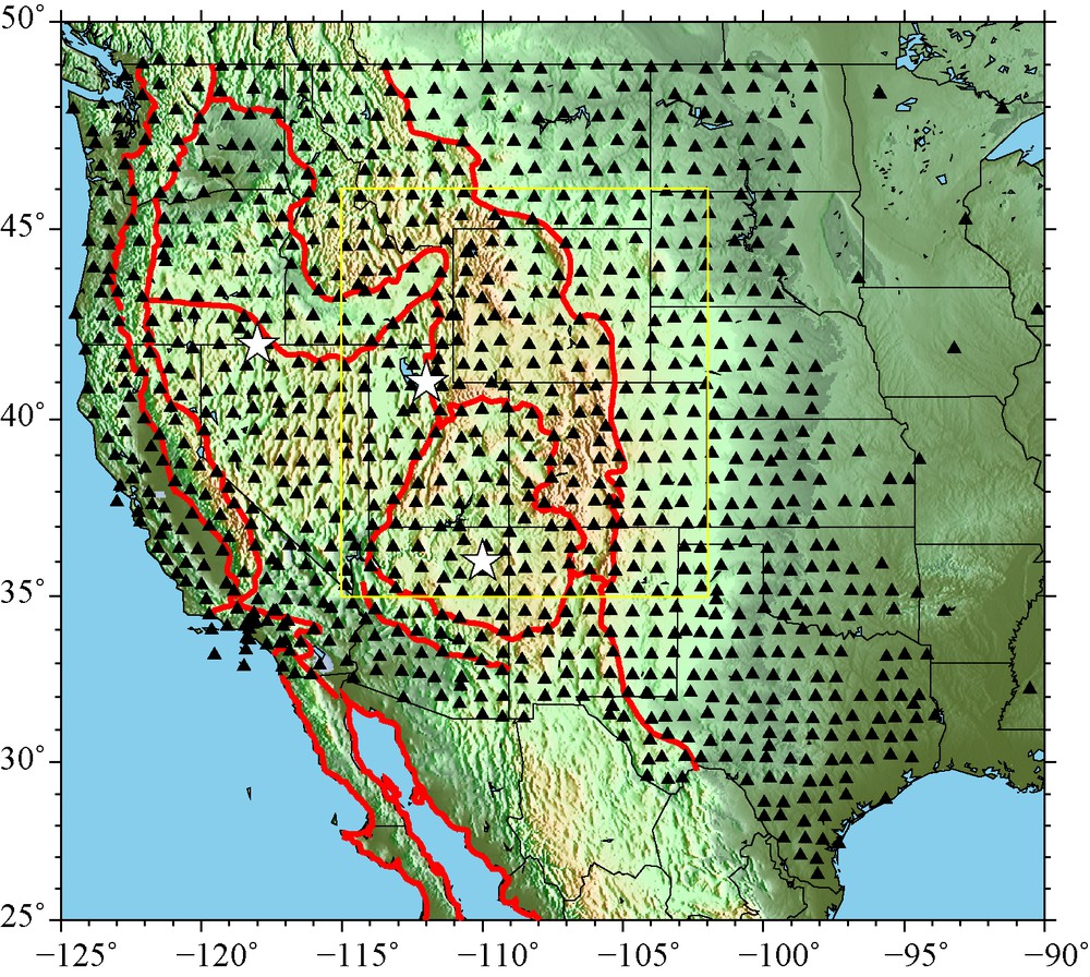
There are 1021 EarthScope USArray Transportable Array and Permanent Array stations (black triangles) used in this study. Locations of geographical points for data results presented in the paper are shown with stars, red contours denote tectonic regions, and the yellow rectangle outlines the location of the results shown on Fig. 11.
Il y a 1021 stations des Earthscope USArray, Transportable Array et Permanent Array (triangles noirs) utilisées dans cette étude. Les localisations des points géographiques dont les données sont présentées dans l’article sont représentées par des étoiles. Les contours rouges matérialisent les régions tectoniques, et le rectangle jaune, la zone d’où proviennent les résultats présentés sur la Fig. 11.
The ambient noise array methods that are discussed here still are based on the computation of EGFs between every pair of stations in the array and the measurement of inter-station phase travel times as a function of period (Bensen et al., 2007). Time domain (Bensen et al., 2007) and spatial autocorrelation (Ekström et al., 2009) methods yield similar travel time estimates (Tsai and Moschetti, 2010). However, for each target station, the set of EGFs to all other stations is used to compute the travel time field of the surface wavefield across a map encompassing the array. In this case, the eikonal equation (Shearer, 2009) can be used to estimate the wave slowness and apparent direction for every location on the map. At each location and frequency, measurements from different target stations can be combined to estimate the azimuthal dependence of the wave speed, which allows an estimate of isotropic and azimuthally anisotropic velocities with rigorous uncertainties. We refer to this procedure as “eikonal tomography” (Lin et al., 2009) because of its basis in the eikonal equation. Eikonal tomography is described in section 2, as are results of its application to data from the EarthScope USarray across the western US. Examples of 3D Vs model results across the western US determined from ambient noise are contained in section 3.
There are several advantages of eikonal tomography compared with traditional tomographic methods (Barmin et al., 2001). Eikonal tomography accounts for ray bending but is not iterative, naturally generates uncertainties at each location in the tomographic maps, provides a direct (potentially visual) means to evaluate the azimuthal dependence of wave speeds, applies no ad hoc regularization because no inversion is performed, and is computationally very fast. There are approximations, however. The method is based on 2D wave propagation stemming from its background in the 2D wave equation, discards a term from the equation that accounts for finite frequency effects, and the method is essentially ray theoretic. We present evidence in section 4 that discarding the amplitude dependent term to derive the eikonal equation is justified at the periods where ambient noise tomography is typically performed (< 40 s). The theoretical background for many of the results presented here is described in greater detail by Lin et al. (2009, 2011a) and Lin and Ritzwoller (in press a,b).
2 Eikonal tomography
Shearer (2009) shows that from the 2D scalar wave equation, the modulus of the gradient of the wave travel time
| (1) |
| (2) |
The eikonal tomography method is based on computing the gradient of the observed travel time surfaces,
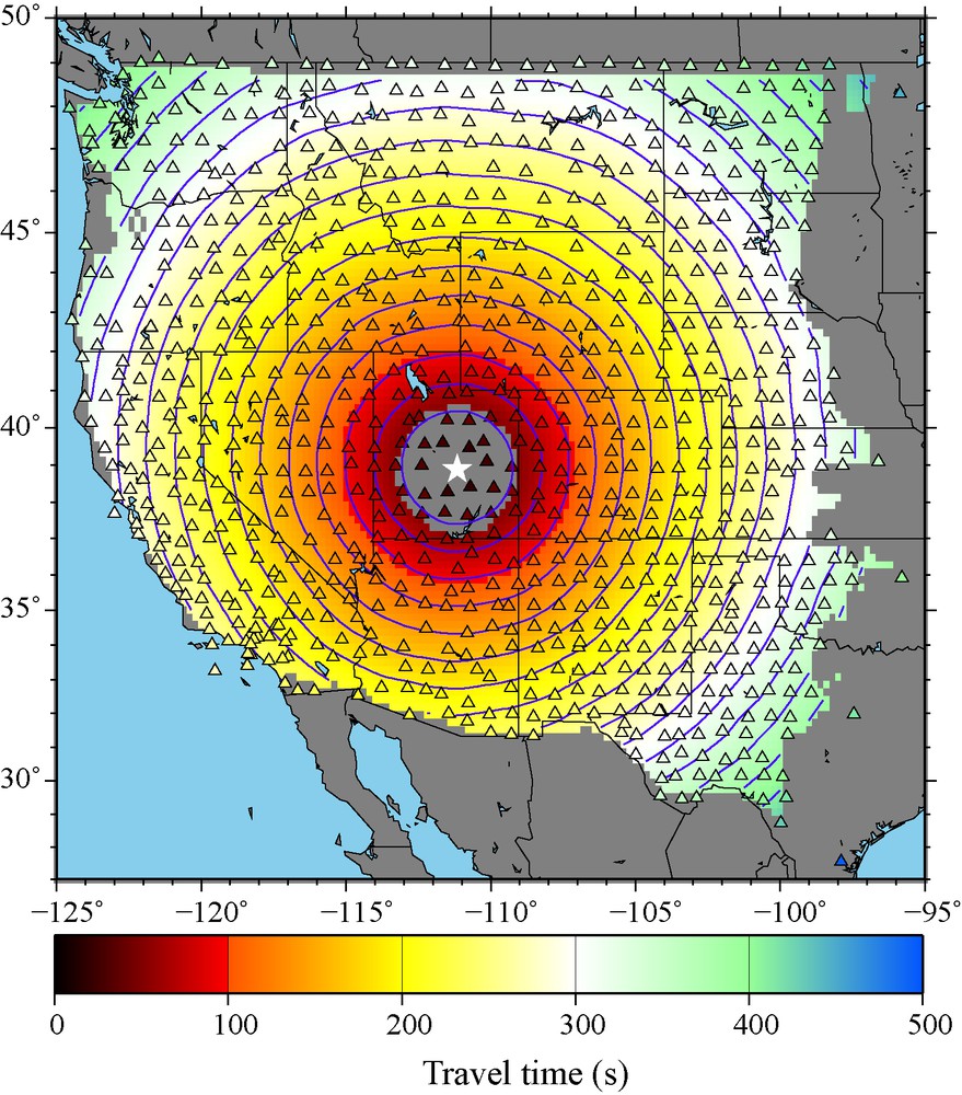
The 24 s Rayleigh wave phase travel time surface computed from ambient noise empirical Green's functions across the western US based on central station (USArray, Transportable Array) Q16A in Utah. Travel time lines are presented in increments of wave period. The map is truncated within two wavelengths of the central station and where the travel times are not well determined. Station Q16A operated simultaneously with the 843 stations shown, but only for a short time near the western and eastern boundaries of the map. Masquer
The 24 s Rayleigh wave phase travel time surface computed from ambient noise empirical Green's functions across the western US based on central station (USArray, Transportable Array) Q16A in Utah. Travel time lines are presented in increments of wave period. The ... Lire la suite
Surface d’isovaleur des temps de trajet de la phase d’onde de Rayleigh à 24 s, calculée d’après les fonctions de Green empiriques du bruit ambiant, à travers l’Ouest des État-Unis, et basée sur la station centrale Q16A dans l’Utah (USArray, Transportable Array). Les lignes de valeur du temps de trajet sont présentées par incrémentation d’une période de l’onde. La carte est tronquée dans deux longueurs d’onde autour de la station centrale et là où les trajets temporels ne sont pas bien déterminés. La station Q16A fonctionne simultanément avec les 843 présentées, mais seulement pour une période courte près des limites occidentale et orientale de la carte. Masquer
Surface d’isovaleur des temps de trajet de la phase d’onde de Rayleigh à 24 s, calculée d’après les fonctions de Green empiriques du bruit ambiant, à travers l’Ouest des État-Unis, et basée sur la station centrale Q16A dans l’Utah (USArray, ... Lire la suite
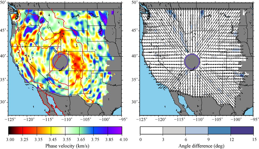
The local (a) phase speed and (b) ray direction inferred from the gradient of the 24 s period Rayleigh wave travel time map shown on Fig. 2 for central TA station Q16A. In (b), the angular difference between the observed and radial directions is shown with the background colour.
Vitesse locale de phase (a) et (b) direction du rayonnement déduite du gradient de la carte de trajet temporel de l’onde de Rayleigh à la période de 24 s, présentée sur la Fig. 2, pour la station centrale TA Q16A. En (b), la différence entre directions radiales et observées est matérialisée par la couleur du fond de la figure.
To estimate azimuthal anisotropy for each location, all measurements from the nine nearby grid nodes with 0.6°C separation (3 × 3 grid with target point at the centre) are combined to estimate the azimuthal variation of the phase speeds. This is shown for two locations in Fig. 4 in which measured speeds are averaged in each 20°C azimuthal bin and plotted as 1σ (standard deviation) error bars. These error bars derive from the scatter in the measurements across nine adjacent grid nodes and provide a rigorous estimate of the random component of uncertainty in the phase speed as a function of azimuthal angle ψ. Based on theoretical expectations for a weakly anisotropic medium (Smith and Dahlen, 1973) and the observation of 180° periodicity in the azimuthally dependent phase speed measurements (e.g., Fig. 4), we fit, as a function of position and frequency, the following functional form to the observed variation of wave speed with azimuth
| (3) |
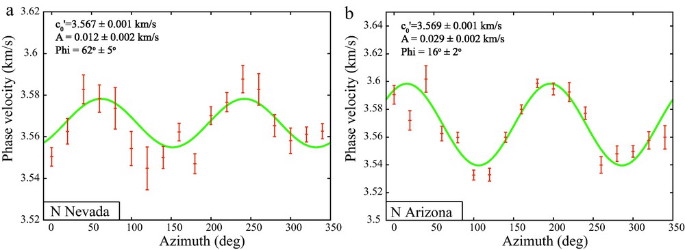
Phase speeds as a function of azimuthal angle and averaged in each 20° bin for the 24 s Rayleigh wave are plotted as 1σ (standard deviation) error bars for example points in (a) Nevada (242°E, 42°N) and (b) Arizona (250°E, 36°N), identified with stars on Fig. 1. The best-fitting 2ψ curve (Eq. (3)) is presented as the green line in each panel. Estimated values with 1 standard deviation errors for
Phase speeds as a function of azimuthal angle and averaged in each 20° bin for the 24 s Rayleigh wave are plotted as 1σ (standard deviation) error bars for example points in (a) Nevada (242°E, 42°N) and (b) Arizona (250°E, 36°N), ... Lire la suite
Les vitesses de phase en tant que fonction de l’azimut, et moyennées tous les 20° pour l’onde de Rayleigh à 24 s sont représentées avec des barres d’erreurs d’1σ (écart type) pour des points choisis au Nevada (242°E, 42°N) et en Arizona (250°E, 36°N) et matérialisés par des étoiles sur la Fig. 1. La courbe 2ψ de meilleur ajustement (Eq. (3)) est représentée, dans chaque panneau, par la ligne verte. Les valeurs estimées, avec des erreurs d’un écart type, pour
Les vitesses de phase en tant que fonction de l’azimut, et moyennées tous les 20° pour l’onde de Rayleigh à 24 s sont représentées avec des barres d’erreurs d’1σ (écart type) pour des points choisis au Nevada (242°E, 42°N) et en ... Lire la suite
When measurements of phase slowness and propagation direction are taken simultaneously from all of the stations across USArray, much more stable results emerge than those that appear in Fig. 3a. For example, the 24 s Rayleigh wave isotropic phase speed map (c0) is shown in Fig. 5a and the amplitudes (A) and fast directions (φ) of the 2ψ component of anisotropy are shown in Fig. 5b. Figs. 3a and 5a should be contrasted. No explicit smoothing or damping has been applied in constructing Fig. 5a. The greater smoothness of Fig. 5a compared with Fig. 3a results from averaging all the measurements at each point (from different central stations) over azimuth. Spatial variations of the azimuthal anisotropy are also smooth and amplitudes typically rise only to several percent. Examples of uncertainties in the variables (c0, A, and φ) are shown in map form for the 24 s Rayleigh wave in Fig. 6. These matters are described in greater detail by Lin et al. (2009).
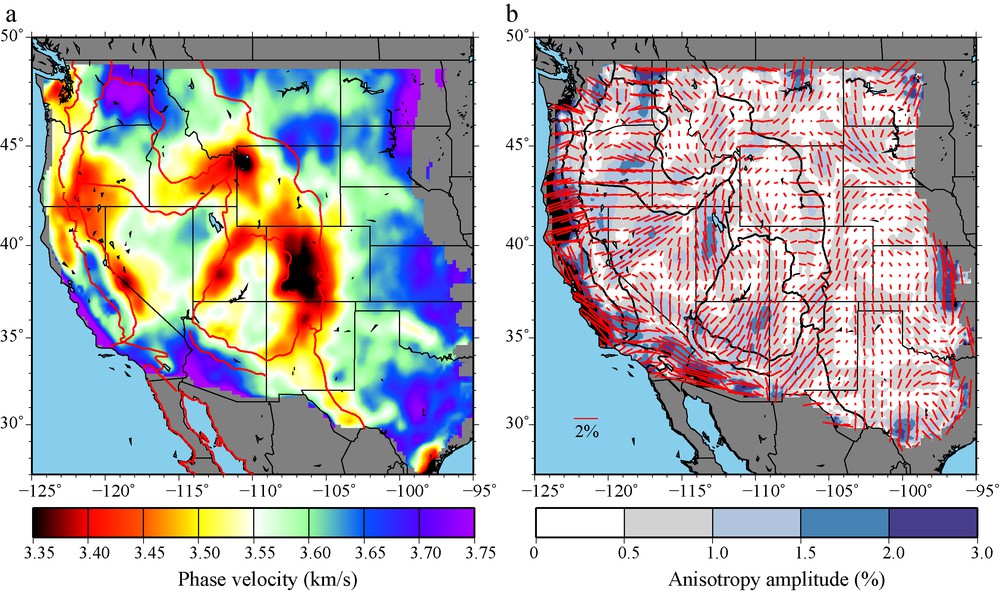
(a): the 24 s Rayleigh wave isotropic phase speed map taken from ambient noise by averaging all local phase speed measurements at each point on the map; (b): the amplitudes and fast directions of the 2ψ component of the 24 s Rayleigh wave phase velocities. The amplitude of anisotropy is identified with the length of the bars, which point in the fast-axis direction, and is colour-coded in the background. At 24 s period, Rayleigh wave anisotropy reflects conditions in a mixture of the crust and uppermost mantle. Masquer
(a): the 24 s Rayleigh wave isotropic phase speed map taken from ambient noise by averaging all local phase speed measurements at each point on the map; (b): the amplitudes and fast directions of the 2ψ component of the 24 s ... Lire la suite
(a) : carte de vitesse de phase isotrope de l’onde de Rayleigh à 24 s, obtenue à partir du bruit ambiant, en moyennant toutes les mesures locales de vitesse de phase à chaque point de la carte ; (b) : amplitudes et directions rapides de la composante 2ψ des vitesses de l’onde de Rayleigh à 24 s. L’amplitude de l’anisotropie est déterminée par la longueur des barres qui pointent dans la direction d’axe rapide, et est indiquée en couleur dans le fond de la figure : à la période de 24 s, l’anisotropie de l’onde de Rayleigh reflète des conditions de mélange de la croûte et de la partie la plus externe du manteau. Masquer
(a) : carte de vitesse de phase isotrope de l’onde de Rayleigh à 24 s, obtenue à partir du bruit ambiant, en moyennant toutes les mesures locales de vitesse de phase à chaque point de la carte ; (b) : amplitudes et directions rapides ... Lire la suite
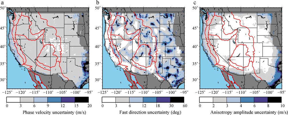
Uncertainties in (a) the isotropic Rayleigh wave phase speed in metre per second, (b) the 2ψ fast-axis direction in degrees, and (c) the amplitude of the 2ψ component of anisotropy (in m/s) for the 24 s Rayleigh wave. Uncertainties are estimated at each point based on the scatter of measurements over azimuth and by fitting Eq. (3) to results such as those shown on Fig. 4.
Incertitudes de la vitesse de phase isotrope de l’onde de Rayleigh en mètre par seconde (a), la direction d’axe rapide 2ψ en degrés (b) et l’amplitude de la composante 2ψ d’anisotropie en mètre par seconde (c), pour l’onde de Rayleigh à 24 s. Les incertitudes sont estimées à chaque point, en se basant sur la dispersion des mesures sur l’azimuth et par l’ajustement de l’Eq. (3) aux résultats tels que ceux présentés sur la Fig. 4.
3 Inversion for isotropic and azimuthally anisotropic 3D Vs models
Isotropic and azimuthally anisotropic dispersion maps and uncertainties, such as those shown in Figs. 5 and 6, provide data to infer a 3D model of shear wave speeds within the earth. The vertical resolution and depth extent of the model will depend on the frequency band of the measurements. Ambient noise tomography typically produces maps to periods as short as 6 to 8 s, although shorter period maps have been constructed in some studies (Yang et al., 2011). This means that structures in the shallow crust (top 5–10 km) can be resolved. Ambient noise tomography, however, rarely extends to periods above 30 to 40 s at regional scales, although long baseline measurements do extend to much longer periods (Bensen et al., 2008, 2009). The variation of the azimuthally dependent phase speed measurements increases dramatically at the longer periods. Thus, ambient noise alone typically constrains structures only to depths of 50 to 80 km. Deeper structures must be constrained with dispersion information from earthquakes as shown, for example, by Lin and Ritzwoller (in press b), Lin et al. (2011a), Moschetti et al. (2010a, 2010b) and Yang et al. (2008b).
Examples of Rayleigh wave phase speed maps from ambient noise at periods of 10 s and 30 s are shown in Fig. 7. Some of the features revealed by these maps have been observed before and were discussed previously by Lin et al. (2008), Moschetti et al. (2010a, 2010b), and Lin et al. (2011a). But the maps in Fig. 7 extend east of the Rocky Mountains, which now reveals new information about the transition from the tectonically deformed western US to the stable mid-continent region. Comparison with similar maps constructed using teleseismic earthquakes, such as those shown in Fig. 7c,f, plays an important role in establishing the reliability of the maps derived from ambient noise, both for isotropic (Yang and Ritzwoller, 2008) and azimuthally anisotropic variables. The 30 s period isotropic Rayleigh wave speeds in Fig. 7b (ambient noise) and Fig. 7c (earthquakes) differ on average by less than 0.1%, where the earthquake derived map is slightly faster, but the difference diminishes systematically as the number of earthquakes increases. The rms difference between these two isotropic maps is about 1%. The rms difference between the fast directions of azimuthal anisotropy determined from ambient noise and earthquakes for the 30 s map is about 25° and the standard deviation of differences in the amplitude of anisotropy is about 0.6%.
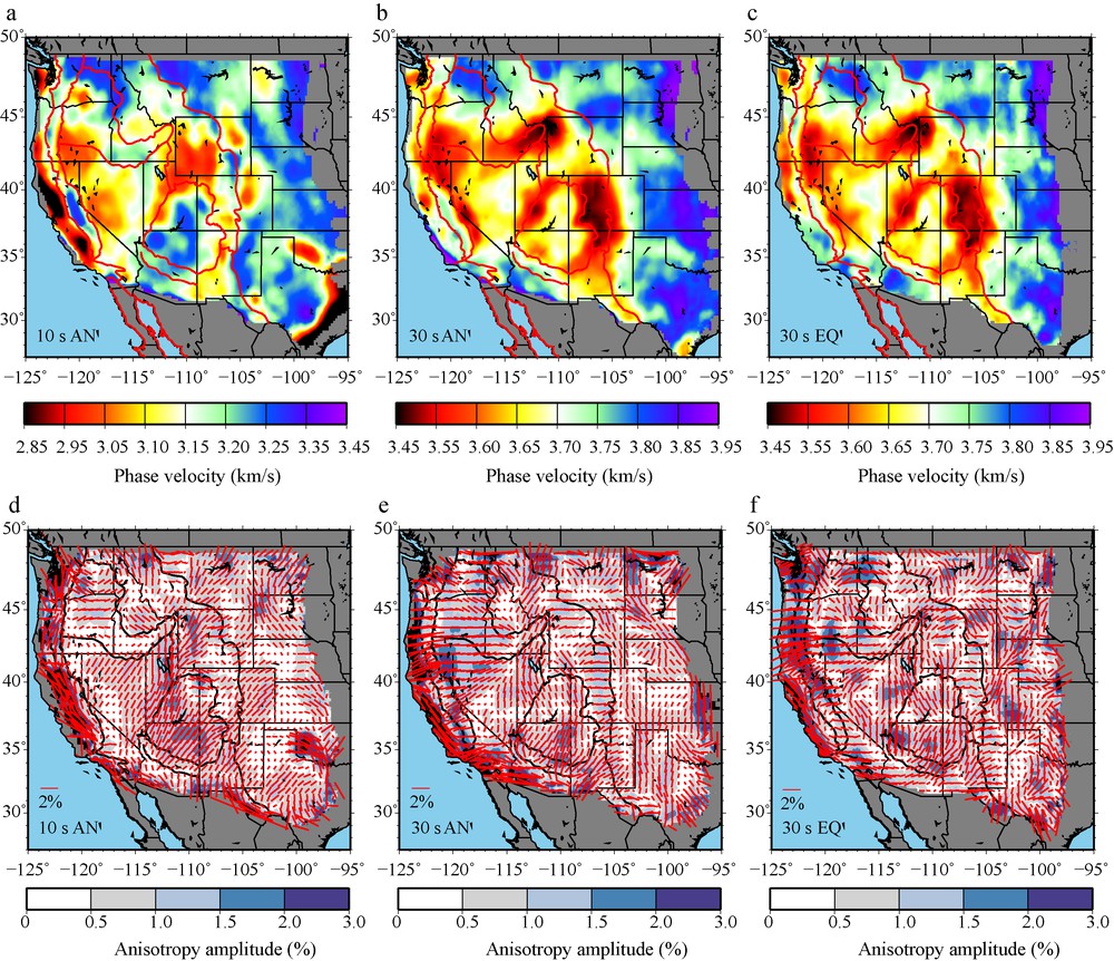
(a) and (b): isotropic maps for the 10 s and 30 s period Rayleigh wave phase speed observed via eikonal tomography applied to ambient noise by averaging all measurements at each location, similar to Fig. 5a; (d) and (e): azimuthal anisotropy from ambient noise also at 10 s and 30 s period, similar to Fig. 5b; (c) and (f): maps of the isotropic Rayleigh wave speed and azimuthal anisotropy at 30 s period observed from teleseismic earthquakes via eikonal tomography (Lin and Ritzwoller, in press a), presented for comparison with (b) and (e). Masquer
(a) and (b): isotropic maps for the 10 s and 30 s period Rayleigh wave phase speed observed via eikonal tomography applied to ambient noise by averaging all measurements at each location, similar to Fig. 5a; (d) and (e): azimuthal anisotropy ... Lire la suite
Cartes isotropes (a) et (b) de la vitesse de phase de l’onde de Rayleigh à 10 s et 30 s, observée par tomographie de l’eikonal, appliquée au bruit ambiant, en moyennant toutes les mesures à chaque localisation, comme en Fig. 5a ; (d) et (e) : anisotropie azimuthale à partir du bruit ambiant pour les périodes 10 s et 30 s, comme sur la Fig. 5b ; (c) et (f) : cartes de vitesse de l’onde isotrope de Rayleigh et d’anisotropie azimuthale à la période de 30 s, observées à partir de tremblements de terre télésismiques par tomographie de l’eikonal (Lin et Ritzwoller, sous presse a), présentées pour comparaison avec (b) et (e). Masquer
Cartes isotropes (a) et (b) de la vitesse de phase de l’onde de Rayleigh à 10 s et 30 s, observée par tomographie de l’eikonal, appliquée au bruit ambiant, en moyennant toutes les mesures à chaque localisation, comme en Fig. 5a ; ... Lire la suite
At 10 s period, several sedimentary basins clearly appear east of the Rocky Mountains: the Permian Basin in west Texas, the Anadarko Basin east of the Texas Panhandle, the Denver Basin in eastern Colorado, the Powder River Basin in eastern Wyoming, and the Williston Basin in western North Dakota. Although this region is on average faster than the western US, the maps display significant variability in the Great Plains even at 30 s period. Most of this variability at 30 s period is due to variations in crustal structure and thickness, which heretofore has been poorly understood. Love wave maps also have been constructed (Lin et al., 2008; Moschetti et al., 2010a), but are not shown here.
Both linearized (Yang et al., 2008a, 2008b) and Monte-Carlo (Lin et al., 2011a; Moschetti et al., 2010a, 2010b; Shapiro and Ritzwoller, 2002) methods to invert local Rayleigh and Love wave dispersion curves for a 3D Vs model are now well established. Example local dispersion curves for a point in northern Nevada are presented in Fig. 8. These include the anisotropic dispersion curves (Fig. 8b,c) discussed by Lin et al. (2011a). In these curves, below 25 s period ambient noise measurements are used alone, between 25 s and 45 s period, ambient noise and earthquake measurements are averaged, and above 45 s period earthquake measurements are used alone. At this location and many others across the western US, measurements of Rayleigh wave anisotropic amplitude and fast direction differ between short and long periods. This indicates that anisotropy differs between the crust and uppermost mantle, but these curves can be fit by a model in which crustal and uppermost mantle anisotropy are simple but distinct. Examples of crustal and uppermost mantle isotropic Vs wave speeds and azimuthal anisotropy are shown in Fig. 9, which is discussed in detail by Lin et al. (2011a). Uncertainty estimates for these model parameters derive from the Monte-Carlo inversion.
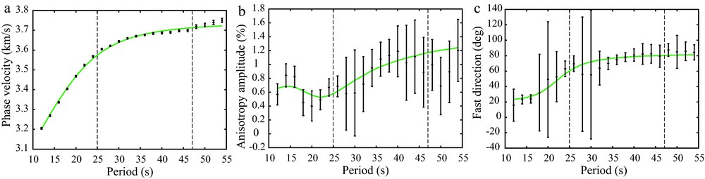
Isotropic and azimuthally anisotropic dispersion curves in northern Nevada for the location shown with a star in Fig. 1. Only ambient noise measurements are used at periods below 25 s, ambient noise and earthquake measurements are averaged between 25 s and 45 s period, and only earthquake measurements are used above 45 s period. Phase velocity is presented in km/s, anisotropy amplitude in percent, and the fast direction of anisotropy in degrees east of north. Measurement uncertainties are presented with one standard deviation error bars. Additional scaling as described in Lin et al. (in press) is applied to the uncertainties of anisotropy measurements based on the misfit to the data by Eq. (3). The best-fitting curves based on the isotropic and anisotropic inversions are presented as the continuous line in each panel. Masquer
Isotropic and azimuthally anisotropic dispersion curves in northern Nevada for the location shown with a star in Fig. 1. Only ambient noise measurements are used at periods below 25 s, ambient noise and earthquake measurements are averaged between 25 s and ... Lire la suite
Courbes de dispersion isotrope et azimuthalement anisotrope dans le Nord du Nevada, repéré par une étoile sur la Fig. 1. Seules les mesures de bruit ambiant sont utilisées aux périodes de moins de 25 s, les mesures de bruit ambiant et de tremblements de terre sont moyennées pour les périodes entre 25 et 45 s, et seules les mesures de tremblements de terre sont utilisées pour les périodes de plus de 45 s. La vitesse de phase est donnée en km/s, l’amplitude de l’anisotropie en pourcent, et la direction rapide d’anisotropie en degrés vers l’est depuis le nord. Les incertitudes dans les mesures sont présentées par des barres d’erreur d’un écart type. Une normalisation additionnelle, comme celle décrite par Lin et al. (in press) est appliquée aux incertitudes des mesures d’anisotropie, basées sur leur inadaptation aux données par rapport à l’Eq. (3). Les courbes de meilleur ajustement, basées sur les inversions isotropes et anisotropes sont représentées par une ligne dans chaque panneau. Masquer
Courbes de dispersion isotrope et azimuthalement anisotrope dans le Nord du Nevada, repéré par une étoile sur la Fig. 1. Seules les mesures de bruit ambiant sont utilisées aux périodes de moins de 25 s, les mesures de bruit ambiant ... Lire la suite
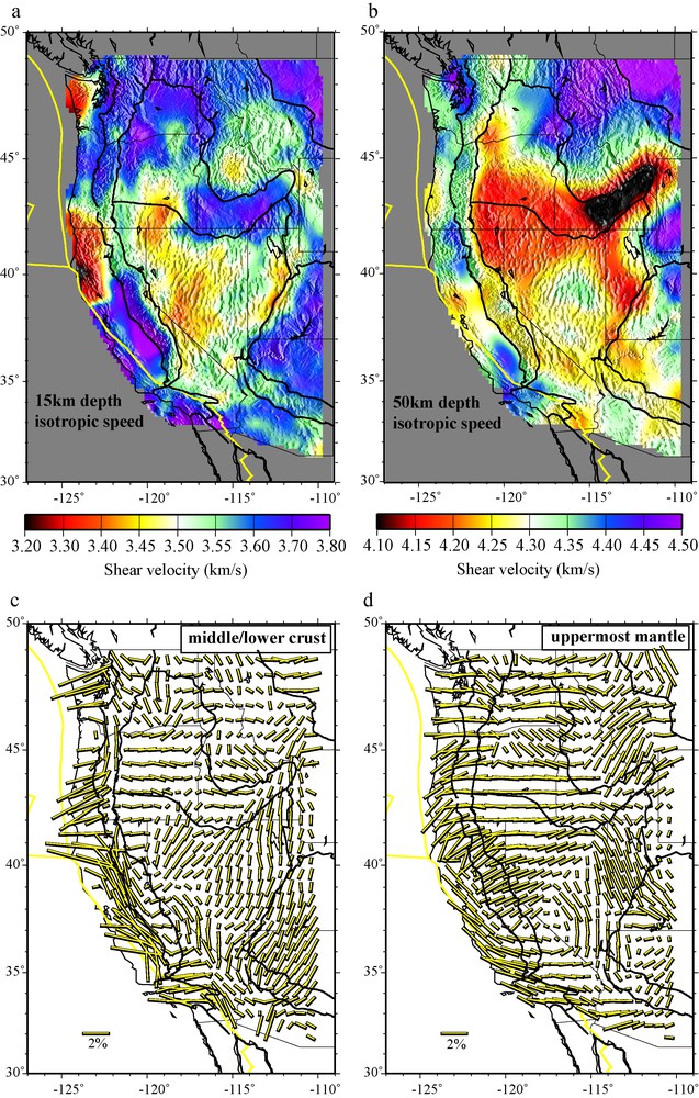
3D model results: (a): isotropic Vs velocity in the crust; (b): isotropic Vs velocity in the uppermost mantle; (c): azimuthal anisotropy in the middle to lower crust; and (d): anisotropy in the uppermost mantle. Results are taken from the model of Lin et al. (2011a).
Résultats du modèle 3D : (a) : vitesse isotrope Vs dans la croûte ; (b) : vitesse isotrope Vs dans le manteau supérieur ; (c) : anisotropie azimuthale dans la partie moyenne et inférieure de la croûte ; (d) : anisotropie dans le manteau supérieur. Les résultats sont extraits du modèle de Lin et al. (2011a).
4 The effect of approximations
The derivation of the eikonal equation, Eq. (2), involves discarding the Laplacian term ∇2A / Aω2. This may be justified by considering it to be a ray theoretic (high frequency) approximation, but may also be valid if the amplitude field were sufficiently smooth; for example, if the length scale of the tomography is sufficiently large or isotropic structures are sufficiently smooth in the region. Thus, for global scale applications, rejection of this term may be justified. But, in ambient noise tomography, spatial length-scales are typically regional or local, not global (This is also increasingly true in earthquake studies; Lin and Ritzwoller, in press a,b; Pollitz, 2008; Pollitz and Snoke, 2010; Yang and Forsyth, 2006; Yang et al., 2008b). For this reason, in ambient noise tomography, the validity of the rejection of the Laplacian term will depend on the local smoothness of the medium and also will be frequency dependent.
To determine the relative size of the Laplacian term compared with the first (gradient) term on the right of Eq. (1), it would be best to compute it from amplitude observations just as the gradient term is computed from travel time observations. This is not so simple, however. In processing ambient noise (Bensen et al., 2007), amplitudes are typically normalized in the time domain by a running mean or one-bit normalization and spectra are commonly whitened. In addition, the amplitude of the ambient noise wavefield is neither isotropic nor stationary, but depends on excitation that varies with azimuth and season. Although, in principle, processing artifacts can be overcome or circumvented (Lin et al., in press; Prieto et al., 2009), doing so is beyond the scope of this paper.
The rejection of the Laplacian term, however, has an effect on apparent phase (or travel time) information that can be discerned in the observed azimuthal distribution of apparent phase speeds. Lin and Ritzwoller (in press a) discuss this in detail for earthquake data and show that discarding this term introduces an apparent 1ψ bias in the azimuthal distribution of phase speeds in regions with strong lateral structural gradients. Although their discussion is for earthquake waves, the physical significance of the Laplacian term is the same for ambient noise wavefields. Thus, observation of a 1ψ term in the azimuthal distribution of phase speeds is evidence that the Laplacian term may be important for the fidelity of both the isotropic and anisotropic components of local phase velocity. Conversely, lack of observation of a 1ψ component is evidence that the Laplacian term and, thus, isotropic bias of inferred anisotropy is small and the use of the eikonal equation is justified.
Lin and Ritzwoller (in press a) discuss how backscattering near strong structural contrasts causes the 1ψ term. The details of the effect will depend on the shape of the anomaly, so smaller bias terms may also exist for the 0ψ, 2ψ, 3ψ, etc. components of local phase speed as Bodin and Maupin (2008) discuss. To diagnose the presence of a 1ψ term, we modify Eq. (3) to include the term
Fig. 10 presents examples of the apparent distribution of phase speed as a function of azimuth for periods of 10 s, 30 s, and 60 s for a point in northern Utah based on eikonal tomography with ambient noise measurements. At 10 s and 30 s periods, only the 2ψ component is strong. However, at 60 s period, in addition to larger error bars due to the stronger scatter caused by lower signal-to-noise ratio at longer periods for ambient noise, the 1ψ component is dominant and is much stronger than the 2ψ component at any period. While lower signal-to-noise ratios at longer periods can prevent the extraction of meaningful 2ψ azimuthal anisotropy information, the existence of strong 1ψ signal is evidence of systematic bias in estimates of both isotropic and anisotropic variables. The size of the observed 1ψ component across the centre of our study region, where we have measurements from all azimuths and isotropic structures are particularly complex, is shown on Fig. 11 at several periods. The amplitude of this component is small at 10 s and 30 s period even though isotropic anomalies are strong. At 60 s period, however, the 1ψ component has a large amplitude surrounding many of the prominent isotropic velocity anomalies (Fig. 11c,f). Around low velocity anomalies, such as the Snake River Plain anomaly seen in the 60 s map in Fig. 11c, the fast directions of the 1ψ component point radially outward from the isotropic anomaly. Around high velocity anomalies, such as that in Wyoming (Fig. 11c), the fast directions of the 1ψ component point radially inward toward the isotropic anomaly. This provides the diagnosis that the 1ψ signal arises from backscattering in the neighbourhood of a velocity contrast.
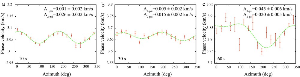
Rayleigh wave phase speeds determined from ambient noise as a function of azimuthal angle and averaged in each 20° azimuthal bin are plotted as 1σ (standard deviation) error bars at periods of 10 s, 30 s, and 60 s for the point in northern Utah shown with a star on Fig. 1. The green dashed line is the best fitting 1ψ and 2ψ curve. The 1ψ component is small at periods below ∼40 s, but dominates the azimuthal dependence of phase velocities at 60 s period. The 1ψ component is spurious, resulting from the apparent phase velocity increase or decrease caused by backscattering near the station. Masquer
Rayleigh wave phase speeds determined from ambient noise as a function of azimuthal angle and averaged in each 20° azimuthal bin are plotted as 1σ (standard deviation) error bars at periods of 10 s, 30 s, and 60 s for the point ... Lire la suite
Les vitesses de phase de l’onde de Rayleigh, déterminées à partir du bruit ambiant comme une fonction de l’angle azimuthal et moyennées tous les 20° sur l’azimuth, sont représentées avec des barres d’erreur d’1σ (déviation standard) pour les périodes 10, 30 et 60 s sur l’exemple du Nord de l’Utah matérialisé par une étoile sur la Fig. 1. La ligne verte en tiretés représente le meilleur ajustement des courbes 1ψ et 2ψ (Eq. (3)). La composante 1ψ est faible pour les périodes au-dessous de 40 s, mais domine la dépendance azimuthale de vitesses de phase pour la période de 60 s. La composante 1ψ est parasite, résultant de la croissance ou de la décroissance apparente de la vitesse de phase causée par la rétrodiffusion près de la station. Masquer
Les vitesses de phase de l’onde de Rayleigh, déterminées à partir du bruit ambiant comme une fonction de l’angle azimuthal et moyennées tous les 20° sur l’azimuth, sont représentées avec des barres d’erreur d’1σ (déviation standard) pour les périodes 10, ... Lire la suite
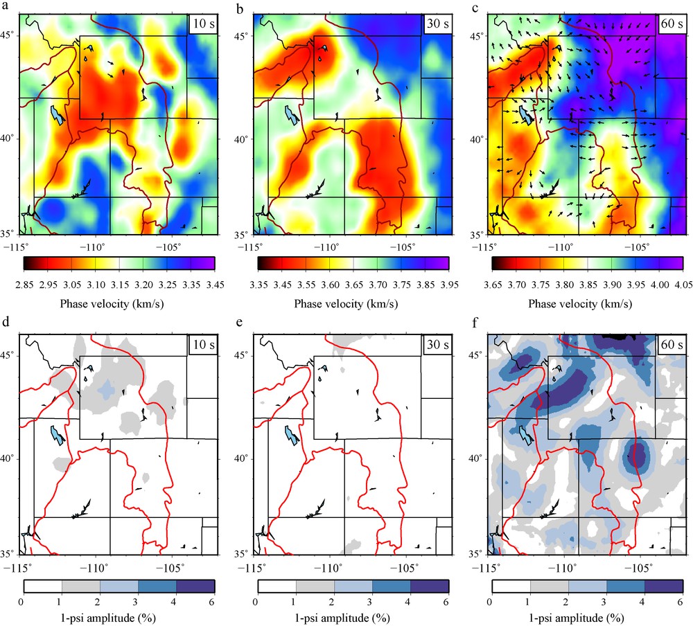
(a)–(c): maps of isotropic Rayleigh wave speeds at 10 s, 30 s, and 60 s period (presented in km/s) determined from ambient noise where the orientation of the 1ψ component of Rayleigh phase speed is over-plotted with an arrow pointing in the fast-direction. Arrows are plotted only if the peak-to-peak amplitude of the 1ψ component is at least 2%. At 60 s, arrows point away from slow isotropic anomalies and toward fast anomalies. (d)–(f) Amplitude of the 1ψ component of phase speed, presented in percent. Strong amplitudes surround the principal isotropic anomalies at 60 s period. Masquer
(a)–(c): maps of isotropic Rayleigh wave speeds at 10 s, 30 s, and 60 s period (presented in km/s) determined from ambient noise where the orientation of the 1ψ component of Rayleigh phase speed is over-plotted with an arrow pointing in the ... Lire la suite
(a)–(c) : cartes de vitesses isotropes de l’onde de Rayleigh aux périodes de 10, 30 et 60 s (présentées en km/s), déterminées à partir du bruit ambiant. L’orientation de la composante 1ψ de la vitesse de phase de Rayleigh est sur-ajoutée, avec une flèche pointant dans la direction rapide. Les flèches sont représentées seulement si l’amplitude pic-à-pic de la composante 1ψ est au moins de 2 %. À 60 s, les flèches s’écartent des anomalies isotropes lentes et pointent vers les anomalies rapides. (d)–(f) : amplitude de la composante 1ψ de la vitesse de phase, donnée en pourcent. Les fortes amplitudes entourent les anomalies isotropes principales pour la période 60 s. Masquer
(a)–(c) : cartes de vitesses isotropes de l’onde de Rayleigh aux périodes de 10, 30 et 60 s (présentées en km/s), déterminées à partir du bruit ambiant. L’orientation de la composante 1ψ de la vitesse de phase de Rayleigh est sur-ajoutée, avec ... Lire la suite
The observation of a gradual increase of the 1ψ component of Rayleigh wave phase velocities at periods above about 40 s is evidence for systematic bias in estimates of isotropic and anisotropic structures. Thus, above 50 s period, ignoring the Laplacian term in eikonal tomography is invalid in regions with strong lateral gradients in the isotropic wave speeds. Below 40 s period, which is the focus of most ambient noise studies, the 1ψ term is largely negligible, even where structural gradients are exceptionally strong. The introduction of measurements obtained from earthquakes (Lin et al., 2011a) helps to reduce uncertainties in the directionally dependent phase speed measurements and improves the azimuthal coverage particularly near the periphery of the map. It does not mitigate the near-station backscattering effect at periods above 50 s, however (Lin and Ritzwoller, in press a). It is possible and considerably easier to retain the Laplacian term in Eq. (1) for earthquake measurements, because of the loss of amplitude information in obtaining ambient noise measurements. Thus, in the context of regional scale structures such as those resolved in the western US, above 50 s period the Laplacian term in Eq. (1) should be retained to ensure the accuracy of the amplitude of isotropic structures and to minimize bias in the 2ψ component of azimuthal anisotropy. This is done for earthquakes waves by Lin and Ritzwoller (in press b).
5 Conclusions
The development and growth of dense, large-scale seismic continental arrays, such as deployments that are now in place in China, Europe, and the US (e.g., EarthScope USarray), present the unprecedented opportunity to map the substructure of continents at a resolution that appeared to be impossible before their deployment. To capitalize on the investments that these and similar arrays represent, new methods of seismic tomography need to be developed to wring from the arrays more information, better information, and qualitative and quantitative assessments of the accuracy of the information. We present here a discussion of one such method, called eikonal tomography, which is designed to exploit information contained in surface waves that compose ambient noise. We argue that the eikonal tomography method extracts information from ambient noise at high resolution about isotropic wave speeds as well as azimuthal anisotropy at periods from less than 10 s to about 40 s. The information at the short period end of this band often provides unique constraints on crustal structure as surface waves below 20 s period are difficult to observe in many locations with earthquake sources and teleseismic body wave do not determine crustal structures well. In addition, eikonal tomography provides meaningful uncertainty estimates about all measured quantities.
Perhaps the greatest challenge to face new methods designed to exploit the emerging continental arrays will be to mitigate the effects of complexities in the seismic wavefield on the inferred quantities. This is particularly true if relatively subtle influences on the wavefield, such as azimuthal anisotropy, are the intended inferred observable. In particular, wavepath bending or refraction, scattering and multipathing on the way to the array (for teleseismic earthquakes) which are often called non-planar wave effects, wavefield effects within the array (such as wavefront healing and backscattering near an observing station), and azimuthal variations in excitation of the wavefield all can affect the observed phase speed of the wavefield and introduce spurious or apparent effects unless they are accounted for explicitly in the data processing and inversion procedures.
Eikonal tomography explicitly tracks wavefields and, therefore, accounts for wavepath bending that is particularly important near sharp structural contrasts and at short periods. But, it is a ray theoretic method and, therefore, does not model structural or wavefield effects away from the ray. However, by its very nature, the inter-station ambient noise wavefield, in contrast with earthquakes, is free from effects external to the array. Wavefield complexities such as wavefront healing and near-station backscattering potentially are important for ambient noise, however, and eikonal tomography, defined by Eq. (2) here, does not explicitly account for it. We present evidence that below 40 s period imaging methods based on ambient noise can ignore wavefield complexities, such as wavefront healing and near-station back scattering. Above ∼50 s period, however, they become increasingly important both for ambient noise and earthquake wavefields. In this case, eikonal tomography will need to be modified to include the second term in Eq. (1), which is based on the amplitude of the observed wavefield. This Laplacian term is deceptively simple, but it accounts for a wide array of wavefield effects, including wavefield complexities arising within the array (or outside the array for earthquake observations) as well as azimuthal variations in excitation. Its application, however, requires that amplitudes be well defined so that instruments must be well calibrated and processing procedures cannot result in the degradation or loss of information about amplitudes.
The retention of the Laplacian term in Eq. (1) with earthquake data is relatively straightforward and is discussed by Lin and Ritzwoller (in press b). Standard ambient noise data processing, however, typically loses amplitude information. Therefore, to apply eikonal tomography above ∼50 s period and retain the Laplacian term in Eq. (1) will require that these procedures be modified so that, at the very least, the effects of data selection and of various normalizations in the time and frequency domain are understood and can be effectively undone. This is an area of active research and is discussed further by Lin et al. (in press). Another approach to model non-ray theoretic effects would be to employ empirical finite frequency sensitivity kernels. Lin and Ritzwoller (2010) describe such an approach in detail.
Acknowledgments
The authors thank two anonymous reviewers for constructive comments. Instruments [data] used in this study were made available through EarthScope (www.earthscope.org; EAR-0323309), supported by the National Science Foundation. The facilities of the IRIS Data Management System, and specifically the IRIS Data Management Centre, were used for access to waveform and metadata required in this study. The IRIS DMS is funded through the US National Science Foundation (NSF) and specifically the GEO Directorate through the Instrumentation and Facilities Program of the National Science Foundation under Cooperative Agreement EAR-0552316. This work has been supported by NSF grants EAR-0711526 and EAR-0844097.
Vous devez vous connecter pour continuer.
S'authentifier