

1 Introduction
Ambient noise or coda-wave cross-correlation has been used to estimate surface-wave propagation (Green's functions) between receivers (Campillo and Paul, 2003; Shapiro and Campillo, 2004), and therefore has been widely used for surface-wave tomography to investigate crustal structure all over the world (Bensen et al., 2008; Cho et al., 2007; Ekström et al., 2009; Fang et al., 2010; Huang et al., 2010; Lin et al., 2008; Moschetti et al., 2007; Sabra et al., 2005; Saygin and Kennett, 2010; Shapiro et al., 2005; Stehly et al., 2009; Yao et al., 2006, 2008; Zheng et al., 2008; Yang et al., 2007). Most previous ambient-noise studies are restricted to continental regions due to the relative scarcity of seismic measurements from the seafloor. Moreover, land-based ambient-noise studies typically only extract fundamental-mode surface waves, with the notable exceptions of Nishida et al. (2008) and Brooks et al. (2009) who observed higher-mode surface waves in Japan and New Zealand, respectively. Harmon et al. (2007) first applied ambient-noise cross-correlation methods to data recorded by ocean-bottom seismographs (OBSs). They utilized the dispersion characteristics of the fundamental and first higher-mode Rayleigh waves to determine crust and uppermost mantle structure at the GLIMPSE experiment site on 3-8-Myr-old lithosphere at 11–16°S on the East Pacific Rise.
In this study we apply ambient noise analysis to vertical-component broadband data recorded by 28 OBSs deployed at the Quebrada/Discovery/Gofar (QDG) transform faults region on the East Pacific Rise (EPR) south of the equator (Fig. 1A). The ambient-noise cross-correlation functions reveal clear surface (Scholte-Rayleigh) wave propagation between each station pair, both for the fundamental mode in the broad period band 2–30 s and for the first higher mode in the period band 3–7 s. The surface-wave dispersion characteristics are used to invert for the 1-D average shear-velocity structure of the crust and uppermost mantle in this region.

A. Bathymetry (Langmuir and Forsyth, 2007; Pickle et al., 2009) and location of 28 broadband ocean bottom seismometers (OBS) (white triangles) around the Quebrada/Discovery/Gofar (QDG) transform faults region on the eastern Pacific Rise (EPR) south of the equator. In the upper left corner of (A), the red rectangle depicts the location of the OBS array. B–E. Show the ray path coverage for the fundamental-mode phase-velocity measurements at four different periods (4 s, 8 s, 15 s, and 25 s). The blue triangles in (B–E) show the location of the OBS sites. The black line in (A) or the red line in (B–E) shows the location of the EPR mid-ocean ridge and QDG transform faults.
A. Bathymétrie (Langmuir et Forsyth, 2007 ; Pickle et al., 2009) et localisation des 28 ocean bottom seismometers (OBSs) large bande (triangles blancs) autour de la région des failles transformantes Quebrada/Discovery/Gofar (QDG) le long de la dorsale Pacifique Est (EPR) au sud de l’équateur. Dans le coin en haut à gauche de (A), le rectangle rouge montre la localisation du réseau d’OBSs. B–E. Montrent la couverture des rais pour la mesure de la vitesse de phase du mode fondamental pour quatre périodes (4 s, 8 s, 15 s et 25 s). Les triangles bleus dans (B–E) montrent la localisation des OBSs. La courbe noire dans (A) et la rouge dans (B–E) montrent la localisation de la dorsale océanique Pacifique Est et des failles transformantes QDG.
2 Data and analysis
A one-year passive deployment of OBSs was carried out from December of 2007 to January of 2009 at the QDG transform fault system in order to better understand the mechanical processes that control earthquake nucleation and the relative partitioning of seismic and aseismic slip on oceanic transform faults. The QDG transform fault system is located on the equatorial EPR (Lat: 3.6–4.8°S, Lon: 107–102°W; Fig. 1) (McGuire, 2008; Pickle et al., 2009). The vertical-component data from 28 broadband sensors (Guralp CMG-3T seismometers) are used for the ambient noise analysis presented in this paper (Fig. 1A).
2.1 Ambient noise cross-correlation functions
We apply a band-pass filter in four period bands (1–5.5 s, 4.5–10.5 s, 9.5–20.5 s, 19.5–30.5 s) to one-day long data segments (vertical component). Since the seismometers are of identical type, we did not correct for the instrument response. Subsequently, we apply one-bit cross-correlation to the filtered data in each period band (Shapiro and Campillo, 2004) and the obtained cross-correlation is filtered again in the same period band to suppress energy outside this band generated by the non-linear one-bit normalization. The daily CFs in the four period bands are then stacked to form the broad band daily CFs (between 1 and 30.5 s period). Using one-bit cross-correlation directly in a broad period band (e.g., 1–30 s period band) would have resulted in (1) an insufficient removal of earthquake signals in the 10–30 s period band as the noise energy is mainly in the secondary microseism band (5–10 s period band) at the ocean bottom; and (2) a more peaky CF spectrum as using one-bit normalization in narrow bands is a way to whiten the CF. Finally, we sum daily CFs to form the yearly CFs. Fig. 2 shows all yearly CFs band-pass filtered in four period bands: 1–5 s, 5–10 s, 10–20 s, and 20–30 s. Signals associated with surface wave propagation appear clearly in each period band.
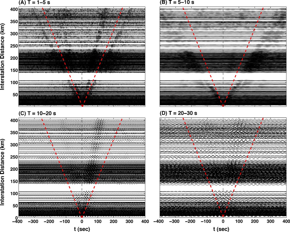
Yearly cross-correlation functions (CFs) for all OBS station pairs in four period bands: (A) 1–5 s; (B) 5–10 s; (C) 10–20 s; and (D) 20–30 s. The positive-time lag CFs correspond to propagation of energy with back azimuth 90–270°, i.e., for station pairs with azimuth between −90° and 90°. The negative-time lag CFs are therefore for station pairs with azimuth between 90° and 270°. The dashed line corresponds to horizontal propagation speed of 1.6 km/s.
Fonctions de corrélation (CFs) annuelles pour toutes les paires d’OBS dans quatre bandes de périodes : (A) 1–15 s ; (B) 5–10 s ; (C) 10–20 s et (D) 20–30 s. Les temps positifs des CFs correspondent à une propagation de l’énergie avec un rétro-azimut entre 90° et 270°, i.e. pour des paires de stations avec un azimut entre −90° et 90°. Les temps négatifs correspondent ainsi à des paires de stations présentant un azimut entre 90° et 270°. La ligne pointillée correspond à une vitesse de propagation horizontale de 1,6 km/s.
Rayleigh waves, which are a type of interface wave propagating along the boundary of an elastic layered medium with a free surface, are commonly observed on the vertical and radial components of land seismic stations (Aki and Richards, 2002). However, in marine (or underwater) seismic experiments with receivers on the seabed, the free surface is replaced by a fluid (water) layer and the interface wave propagating near the fluid-solid interface is usually named a Scholte wave, in contrast with a Rayleigh wave that propagates near the air-solid interface or a Stoneley wave that propagates near a solid-solid interface (Ewing et al., 1957). In marine exploration seismology, Scholte waves are widely used to investigate shallow-water submarine sedimentary structure (see Socco et al. (2010) for a review; Bohlen et al., 2004). In the long-period or long-wavelength limit, the water layer can be neglected and the Scholte wave can be regarded as a Rayleigh wave (Bohlen et al., 2004). However, the surface waves recovered from ambient noise cross-correlation are quite sensitive to the 3 km seawater layer, in particular in the period band 2–10 s. So we call the recovered surface waves (on the vertical component) Scholte-Rayleigh waves throughout the text.
Similar to Harmon et al. (2007), we observe both the fundamental mode and the first higher-mode Scholte-Rayleigh waves in CFs in the 1–5 s and 5–10 s period bands (Fig. 2A and B). The fundamental-mode waves in these two period bands appear time-symmetric. In the 10–20 s and 20–30 s period bands (Figs. 2C and D) we only observe the fundamental mode. In the 10–20 s period band (Fig. 2C) the amplitude of the positive-time CFs is larger than that of the negative-time part, implying more energy propagating from WSW direction. In the 20–30 s period band (Fig. 2D) the CFs are nearly symmetric.
2.2 Dispersion analysis
To enhance the signal to noise ratio of the recovered surface waves and suppress the effect of non-isotropic distribution of noise sources on the recovery of surface-wave Green's function, we stack the positive-time lag CFs and the time-reversed versions of the negative-time lag CFs to form the stacked CFs, which are called the “symmetric component” CFs (Yang et al., 2007). In a 2-D case, when the incidence of the plane waves in a homogeneous elastic medium is isotropic, the CF differs from the real displacement Green's function by a π/2 phase advance (Harmon et al., 2008; Sanchez-Sesma and Campillo, 2006; Tsai, 2009). That is, the phase of the CF equals that of the velocity Green's function (i.e., time derivative of the displacement Green's function). Under the assumption of dominant 2-D plane-wave (surface-wave) incidence (Harmon et al., 2008; Nakahara, 2006), we correct for the π/2 phase shift by taking the Hilbert transform of each symmetric component CF in the time domain in order to obtain the surface wave displacement empirical Green's function (EGFs) between two stations.
Following a traditional frequency-time analysis via the multiple filtering technique (Dziewonski et al., 1969) we construct the velocity-period spectrogram for each EGF and then measure the group-velocity dispersion for the Scholte-Rayleigh wave fundamental and higher modes by picking the peak of the envelope function of the narrow-band filtered signal (Fig. 3). Yao et al. (2006) used the tapered boxcar window within a fixed group-velocity window [v1 v2] (with v1 < v2, e.g., [2 5] km/s) to window the EGF, corresponding to windowing the EGF with the tapered time-domain window within [L/v2 L/v1] with L the propagation distance. For phase-velocity analysis the windowed EGFs were then narrow-band-pass filtered at various frequencies. This is appropriate if the EGF is predominated by fundamental-mode surface waves, but in this study the EGFs within the period band 1–5 s and 5–10 s clearly show both the fundamental mode and the first higher mode surface waves (Fig. 2A, B).

Period-velocity spectrogram (background image) for group velocity dispersion frequency-time analysis (FTAN) from the EGF between the stations D02 and D05. Red and blue colors show for high and low amplitudes, respectively. For each period in the spectrogram, the amplitude has been normalized. The fundamental and the first higher mode group-velocity dispersion curves are shown as the light-blue solid and open circles, respectively. The fundamental and the first higher mode phase velocity dispersion curves for the same path, measured by time-variable filtering analysis, are shown as the green solid and open triangles, respectively.
Spectrogramme période/vitesse (image de fond) utilisé pour l’étude de la dispersion de la vitesse de groupe par analyse temps-fréquence (FTAN) à partir de l’EGF pour les stations D02 et D05. La couleur rouge (resp. bleue) indique une forte (resp. faible) amplitude. L’amplitude est normalisée entre les périodes du spectrogramme. La courbe de dispersion de la vitesse de groupe du mode fondamental (resp. premier mode supérieur) est indiquée par les cercles pleins (resp. vides) bleu clair. La courbe de dispersion de la vitesse de phase du mode fondamental (resp. premier mode supérieur) pour le même trajet, mesurée à l’aide d’une méthode de filtrage à temps variable, est indiquée par des triangles pleins (resp. vides) verts.
In order to avoid contamination of phase-velocity measurements of one surface wave mode by another we adopt a time-variable filtering technique (Landisman et al., 1969) for phase-velocity dispersion analysis. For each period (T) of interest we use a period-dependent (tapered) boxcar window between group velocities [v1(T) v2(T)] to window the EGF in the time domain; subsequently, the windowed EGF for that period of interest is narrow-band-pass filtered using the phase-velocity image-analysis technique (Yao et al., 2006). Based on the average group-velocity dispersion curve obtained for each mode (Fig. 3) we design the group-velocity window [v1(T) v2(T)] for each period and each mode of interest such that it is centered around the signal of one surface wave mode and outside the main signal window of the other mode. With the time-variable filtering technique and phase velocity image analysis we obtain the phase velocity dispersion curve from the EGF for each surface wave mode.
We use the far-field expression of the time harmonic surface wave displacement Green's function to calculate the phase velocities (Appendix A and Yao et al., 2006). The phase difference (travel time difference) between the exact Green's function and the far-field asymptotic Green's function is negligible (less than 0.3%) when propagation distance r > λ, where λ is the wavelength (Appendix A, Fig. A). This estimate is based on the assumption of perfect recovery of the surface-wave Green's function from ambient noise correlation. In reality, however, uneven distribution of ambient noise sources may result in imperfect recovery of the Green's function, and therefore systematic bias of phase velocities (Froment et al., 2010; Harmon et al., 2010; Tsai, 2009; Weaver et al., 2009; Yao and van der Hilst, 2009). This bias tends to increase when r/λ decreases (Tsai, 2009; Yao and van der Hilst, 2009). Therefore, most previous time-domain dispersion measurements from CFs or EGFs require r > 3λ (Lin et al., 2008; Yang et al., 2007; Yao et al., 2006 and many others).
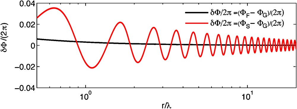
Phase difference per cycle (δΦ/2π) between the far field and the exact Green's function (black line) and between the symmetric component EGF and the exact Green's function (red line), both as a function of r/λ (Appendix A for the detail).
Différence de phase par cycle (δФ/2π) entre la fonction de Green exacte et l’approximation champs lointain d’une part (courbe noire) et l’EGF symétrisée d’autre part (courbe rouge), en fonction de r/λ (Appendix A pour plus de détails).
Due to the relatively short inter-station distances of the OBS array, in this study we require r > 1.5λ in order to obtain dispersion at longer periods, which may help resolve deeper structure. This requirement leads to phase-velocity measurements in a much broader period range for larger inter-station distance. It is often difficult, however, to measure very short-period dispersion (e.g., at T < 5 s) for paths with distances larger than several hundred kilometers due to intrinsic attenuation and scattering (Fig. 1B). Therefore, very large inter-station distance paths usually yield dispersion data for relatively longer periods only (Fig. 1B–E).
Fig. 4 shows the average group- and phase-velocity dispersion curves and their standard deviations for the fundamental mode (period band 2–30 s) and the first higher mode (period band 3–7 s) measured from all inter-station EGFs. The group-velocity dispersion curves show larger standard deviations than the phase-velocity dispersion curves, implying that phase velocity measurements are more accurate. Within the period band 3–7 s, both the fundamental mode and first-higher mode phase velocities are slightly higher than in the GLIMPSE area (Harmon et al., 2007). Within the period band 10–25 s, however, the fundamental-mode phase velocities are lower than for the GLIMPSE area based on ambient noise analysis below 16 s period (Harmon et al., 2007) and also teleseismic surface waves above 16 s period (Weeraratne et al., 2007). This implies that the uppermost mantle shear wavespeed structure is slower in the QDG transform faults region than in the GLIMPSE area.
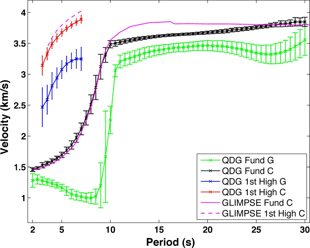
Measured average Scholte-Rayleigh wave phase- (C) and group-velocity (G) dispersion curves and their standard deviation of the fundamental (Fund) and the first higher mode (1st High) from all inter-station paths in the QDG transform faults region. The pink solid and dashed lines show the phase-velocity dispersion curves of the fundamental mode and the first higher mode, respectively, measured at the GLIMPSE study area at 11–16°S on 3–8 Myr-old lithosphere just west of the East Pacific Rise (Harmon et al., 2007; Weeraratne et al., 2007).
Mesure de la dispersion des vitesses de phase (C) et de groupe (G) du mode fondamental (Fund) et du premier mode supérieur (1st High) des ondes de Scholte-Rayleigh, avec les écarts-types associés, pour tous les trajets entre récepteurs dans la région des failles transformantes QDG. La courbe violette continue (resp. pointillée) montre la courbe de dispersion de la vitesse de phase pour le mode fondamental (resp. premier mode supérieur), mesurée pour une lithosphère âgée de 3 à 8 millions d’années dans la zone de l’étude GLIMPSE (11–16°S) située à l’ouest de la dorsale Pacifique Est (Harmon et al., 2007 ; Weeraratne et al., 2007).
3 1-D average velocity structure
The accuracy of the phase-velocity measurements is higher than the group velocity measurements, in particular at longer periods (Bensen et al., 2008), because measuring group velocity from a broad envelope has larger uncertainties than phase velocity measurements. Therefore, we only use the average phase-velocity dispersion data (Fig. 5) to invert for the 1-D average velocity structure (Fig. 1B–E).
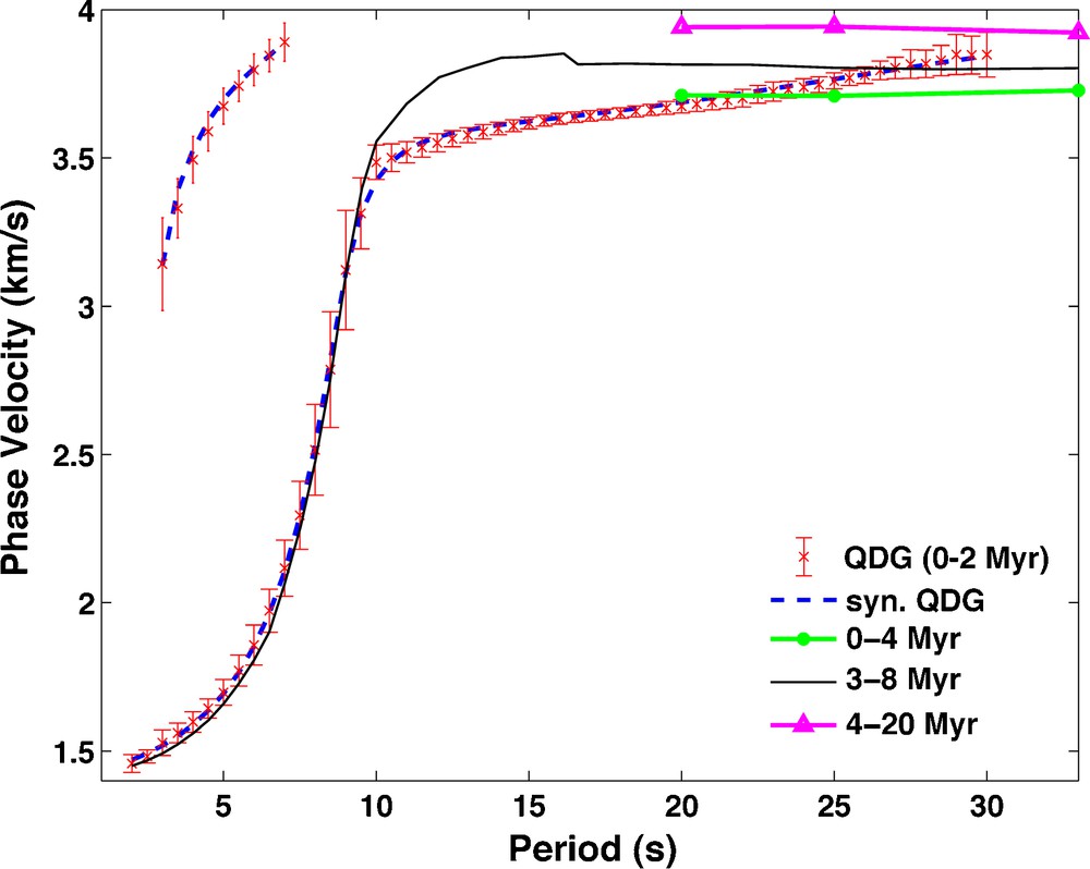
Observed (in red, with error bar) and synthetic (dashed blue) average Scholte-Rayleigh wave phase-velocity dispersion of the fundamental mode and the first higher mode in the QDG transform faults region. The synthetic Scholte-Rayleigh wave dispersion curves are calculated from the posterior mean model of the inversion (the blue Vs profile in Fig. 8). The black, green, and magenta lines show the fundamental-mode phase velocity dispersion data measured at different locations in the Pacific with seafloor ages as indicated. The data shown by the black line is from Weeraratne et al. (2007) and Harmon et al. (2007). The data shown in the green and magenta lines are from Nishimura and Forsyth (1989).
Dispersion de la vitesse de phase des ondes de Scholte-Rayleigh observée (en rouge, avec barres d’erreur) et théorique (en ligne pointillée bleue) pour le mode fondamental et le premier mode supérieur dans la région des failles transformantes QDG. Les courbes de dispersion théoriques des ondes de Scholte-Rayleigh sont calculées à partir du modèle moyen final, après inversion (le profil bleu Vs de la Fig. 8). Les courbes noire, verte et violette montrent la dispersion de la vitesse de phase du mode fondamental, mesurée dans différentes régions de l’océan Pacifique, correspondant à différents âges des fonds océaniques, comme indiqué dans la légende. Les données de la courbe noire proviennent de Weeraratne et al. (2007) et de Harmon et al. (2007). Les données de la courbe verte et violette proviennent de Nishimura et Forsyth (1989).
3.1 Ocean wavespeed and depth
The fundamental-mode Scholte-Rayleigh phase velocities within the period band 2–10 s are mostly sensitive to the ocean acoustic velocity (Vw) and depth (Hw) (Fig. 6; also see Fig. 9 in Harmon et al., 2007). Therefore, it is possible to derive the ocean wavespeed and depth directly from short-period band fundamental mode dispersion data. Because of larger standard deviations in the 8–10 s period band we only use (fundamental-mode) phase velocities within the 2–8 s period band to infer the ocean wavespeed and depth. Since the 2–8 s period phase-velocity measurements from the EGFs have different ray path coverage (Fig. 1B and C) the average phase velocities may be representative of regions with different ocean wavespeed structures and depths. In order to obtain the optimum 1-D model for the entire study region, we perform a grid search for the average ocean Vw and Hw by comparing predicted and observed average fundamental-mode phase-velocity dispersion (Fig. 5) for a given 1-D velocity model consisting of a seawater layer of varying speed and thickness and a fixed crust and upper mantle model from Harmon et al. (2007). The misfit function is defined using an l1 norm as
| (1) |

Scholte-Rayleigh wave phase-velocity (c) sensitivity kernels for Vp (left two plots) and Vs (right two plots) for the fundamental mode (top two plots) and the first higher mode (bottom two plots) at various periods. The velocity model for calculating the sensitivity kernels is the posterior mean shear velocity model (blue line in Fig. 8). The two red lines at depths of 3.3 km and 9.9 km in each plot show the seafloor and Moho interface, respectively. Notice the big differences of the X-axis limits for each subplot, in particular for the fundamental mode (top two plots).
Noyaux de sensibilité aux vitesses Vp (colonne de gauche) et Vs (colonne de droite) de la vitesse de phase (c) du mode fondamental (ligne du haut) et du premier mode supérieur (ligne du bas) des ondes de Scholte-Rayleigh, à différentes périodes. Le modèle de vitesse utilisé pour calculer les noyaux de sensibilité est le modèle de vitesse de cisaillement moyenne finale après inversion (courbe bleue de la Fig. 8). Les deux lignes rouges, correspondant à des profondeurs de 3,3 km et de 9,9 km, indiquent le fond océanique et le Moho. Noter la différence d’échelle des axes des abscisses entre les graphiques, en particulier pour le mode fondamental (ligne du haut).
3.2 Vs in the crust and uppermost mantle
After obtaining the average ocean wavespeed and depth we perform a global search and statistical estimation for the crustal and uppermost-mantle shear velocities using a Neighborhood Algorithm (NA) (Sambridge, 1999a,b; Yao et al., 2008) and the average fundamental mode (period band 2–30 s) and the first higher mode (3–7 s) Scholte-Rayleigh wave phase-velocity dispersion data (Fig. 5). The reference crustal Vs structure consists of a stack of layers with velocities adopted from the GLIMPSE study (Harmon et al., 2007); for the upper mantle we use a constant reference velocity of 4.20 km/s compared to 3.9–4.5 km/s in the GLIMPSE model. The neighborhood search concerns eight parameters: Vs perturbations in the crust, Moho-24.4 km, 24.4–39.4 km, 39.4–54.4, 54.4–69.4 km, and the half space (beneath the sea-surface depth at 69.4 km) with respect to the reference values, Vp/Vs ratio in the crust, and Moho depth (H). For the model space search, we allow perturbations for Vs in the crust and upper mantle layers of ± 0.5 km/s with respect to the reference values. Since the crust is parameterized by a stack of layers with different velocities, the velocity perturbation to the entire crust is made by adding the same shear velocity perturbation to each layer within the crust. Permissible Vp/Vs ratios vary between 1.65 and 1.95, and Moho depth is allowed to deviate 1.5 km from the value measured in the GLIMPSE region; that is, the crustal thickness range is 4.6–7.6 km.
We generally follow Yao et al. (2008) to determine parameters for the neighborhood search. The misfit between the observed and predicted dispersion data is defined using an l1 norm similar to Eq. (1) but includes the average dispersion data for both the fundamental mode (period band 2–30 s at 0.5 s increments) and the first higher mode (3–7 s, 0.5 s increments) (Fig. 5). We emphasize that the standard deviation in equation (1) used to inversely weight the dispersion data in the inversion is not the average error of the measured phase velocities but a measure of the variation of structure within the study region sampled by different inter-station ray paths. The reference Vp in the upper mantle is 1.9 Vs, but upon the search Vp changes along with Vs and Vp/Vs ratio using scaling relationships (Yao et al., 2008). Density in the crust and upper mantle also changes along with Vp and Vs following Yao et al. (2008).
The model ensemble generated during the first step of the NA (Sambridge, 1999a) is used to perform Bayesian analysis to infer the resolution and trade-offs in the model parameters (Sambridge, 1999b). The posterior mean values of the model parameters inferred from the 1-D posterior probability density function (PPDF) are shown as the black lines in Fig. 7. The Vs in the crust and the two uppermost mantle layers (Moho-24.4 km and 24.4–39.4 km) are well resolved and have standard deviations about 0.1 km/s. However, the Vs in the deeper upper mantle layers (39.4–54.4, 54.4–69.4 km, and the half space) are not very well resolved (standard deviations: 0.15–0.2 km/s) due to the limited band width of the data used in the inversion. The posterior mean value of Vp/Vs ratio is 1.80 with a standard deviation of 0.07. The broad non-Gaussian distribution of the PPDF for the perturbation to the crustal thickness suggests that Moho depth is not well resolved by dispersion measurements, which is common for surface wave dispersion inversion due to the relatively broad sensitivity kernel around Moho depth (Fig. 6) and the trade-off between crustal thickness and velocity structure in the lower crust and uppermost mantle (Yao et al., 2008).

The distribution of 1-D posterior probability density function of the 8 model parameters from the NA (Section 3.2). The vertical axes show the normalized probability. The horizontal axes show the perturbation range of each parameter (as indicated) with respect to the reference value, and the black lines give the posterior mean values.
Densité de probabilité 1D a posteriori pour les 8 paramètres de l’algorithme de voisinage (NA, Section 3.2). La probabilité normalisée apparaît en ordonnée. L’axe des abscisses indique la gamme de perturbation autour de la valeur de référence pour chaque paramètre, et la ligne noire indique la valeur moyenne a posteriori.
The final shear-velocity model (Fig. 8) is represented by the mean values and standard deviations of the 1-D PPDFs (Fig. 7). The average crustal velocity for the QDG region is 0.09 km/s higher (2–3%) than the reference model, but is indistinguishable from the reference within the standard error range (3–4%). The average Vs (4.29 km/s) in the uppermost mantle layer (Moho-24.4 km) is 0.1–0.2 km/s less than in the GLIMPSE region (Harmon et al., 2007). We observe a very low velocity layer (with Vs ∼3.85 km/s) within the sub-surface depth range 24.4-39.4 km, which is significantly lower (> 10%) than in the GLIMPSE region (Vs ∼4.35 km/s). Below this low- velocity layer Vs increases with increasing depth, but the standard errors are larger. The predicted dispersion curves (blue lines in Fig. 5) from the 1-D posterior mean shear-velocity model (blue line in Fig. 8) agree with the observed data (green circles in Fig. 5), indicating the robustness of the model obtained from the NA.

The posterior mean shear-velocity model (blue line) and its standard error (shaded region) obtained from the NA (Fig. 7) using dispersion data shown in Fig. 5 (red x). The Vs profile shown by the black line is from Weeraratne et al. (2007) and Harmon et al. (2007), and the green and magenta Vs profiles are from Nishimura and Forsyth (1989). The corresponding dispersion data for these three Vs profiles are shown in Fig. 5.
Modèle moyen a posteriori de la vitesse de cisaillement (courbe bleue) et son écart-type (surface grisée) obtenus grâce à l’algorithme de voisinage (NA, Fig. 7) à partir des données de dispersion de la Fig. 5 (croix rouges). Le profil Vs indiqué par la courbe noire provient de Weeraratne et al. (2007) et de Harmon et al. (2007), et les profils vert et violet de Nishimura et Forsyth (1989). Les courbes de dispersion correspondant à ces trois profils Vs sont tracées sur la Fig. 5.
4 Discussion
4.1 Uncertainties in dispersion data from EGFs
Several factors affect the accuracy and reliability of our dispersion measurements from EGFs. First, strong dispersion due to the sharp increase in the fundamental-mode Scholte-Rayleigh wave group velocity in the period band 8–11 s reduces the energy and the SNR in this band. This could explain the much larger standard deviation (e.g., about 0.22 km/s at 8.4 s period) of the average phase velocity dispersion curve in this period band (Fig. 4). Another reason could be the considerable variations in the average ocean depth along each inter-station path. A forward dispersion calculation shows that a 50 m change in seafloor depth in our final model (Fig. 8) will cause a 1–2% change in Scholte-Rayleigh wave fundamental-mode phase velocities in the period band 6–10 s. Variations in seafloor depth of a few hundred meters along the inter-station paths will result in considerable variations in the dispersion within the 6–10 s period band. However, weighting (upon NA inversion) the data with the inverse of the standard deviation limits contributions of dispersion measurements with large associated errors to the final model. This might occur in particular for the uppermost mantle structure where the Scholte-Rayleigh wave fundamental-mode between 7 and 10 s has little sensitivity (Fig. 6 and Harmon et al., 2007).
An uneven distribution of ambient noise sources may also introduce systematic errors in the dispersion measurements (Froment et al., 2010; Gouédard et al., 2008; Harmon et al., 2010; Tsai, 2009; Weaver et al., 2009; Yao and van der Hilst, 2009). In the shorter period bands (2–10 s) we observe good symmetry between the positive- and negative-time CFs (Fig. 2A and B). This is probably due to good azimuthal distribution of ambient noise sources and strong local scattering of surface waves at higher frequencies due to large variations in bathymetry of the order of the wavelength (Fig. 1). Scattering helps to homogenize the ambient-noise wavefield for better recovery of the Green's function (Malcolm et al., 2004) and hence better measurement of phase velocity. In the primary microseism band (10–20 s) the CFs are not time-symmetric (Fig. 2C), with more energy propagating from WSW direction. However, because we average over one year of data we would expect smooth variations in the ambient noise energy distribution, as reported in previous ambient noise studies (Harmon et al., 2008; Stehly et al., 2006; Yang et al., 2007). Theoretical and numerical studies (Froment et al., 2010; Tsai, 2009; Yao and van der Hilst, 2009) have shown that the errors in dispersion measurements from ambient noise studies are typically very small when the inter-station distances are several wavelengths apart, which explains the success of ambient noise tomography on various length scales. A smooth distribution of ambient noise energy will improve the recovery of Green's functions, and hence suppress errors in dispersion measurements, which are mostly on an order of about 1% even with monthly data (Yao and van der Hilst 2009). In this study, the effect of uneven noise distribution on phase velocity dispersion measurement is expected to be within 1–2%, which is close to or within the standard deviation of our average dispersion curves (Fig. 5). Therefore, the final model and its uncertainty range from the NA inversion (Fig. 8) are considered representative of the true structure of the crust and uppermost mantle across the QDG transform faults area.
4.2 Low-velocity uppermost mantle
The average crustal structure in the QDG transform faults area is similar to the structure in the GLIMPSE region reported by Harmon et al. (2007) (Fig. 8). However, the uppermost mantle at the QDG site (Moho-39.4 km sub-surface depth) is significantly slower. The average shear velocity between Moho and a sub-surface depth of 24.4 km is 4.29 km/s, about 5% less than a global reference value of 4.5 km/s (Kennett et al., 1995). This suggests either that the high-velocity, uppermost mantle lid that is typical for oceanic regions (Gaherty et al., 1996; Nishimura and Forsyth, 1989) is absent in the QDG region or that it is too thin to be resolved by our dispersion measurements. We note that a fast lid also appears absent near the ridge at the MELT experiment site (Dunn and Forsyth, 2003). Moreover, in the depth range of 24.4–39.4 km the average shear velocity is only 3.85 km/s. This low-velocity zone (LVZ) in the uppermost mantle in the QDG region appears about 25–40 km shallower than in the GLIMPSE region (Harmon et al., 2007; Weeraratne et al., 2007) and MELT region (Evans et al., 2005). Several previous studies (Gu et al., 2005; Webb and Forsyth, 1998) found shear velocity of the oceanic upper mantle LVZ from Rayleigh wave inversion can be as low as 3.7 km/s. In the presence of azimuthal seismic anisotropy such low shear velocities can be due to propagation along slow axes, which are parallel to the ridge. Here, however, the direction of ray paths is closer to the ridge spreading direction, or the fast axis of azimuthal anisotropy. The inferred velocity may, thus, be an upper bound, and the isotropic (average) velocity in the upper mantle LVZ beneath the QDG region could be even slower than 3.85 km/s.
The QDG region has a seafloor age about 0–2 Myr, in contrast to 3–8-Myr-old lithosphere of the GLIMPSE region (Weeraratne et al., 2007). In general, older lithosphere is thicker and colder than younger lithosphere, and hence has higher uppermost mantle velocities and a deeper low-velocity zone (Harmon et al., 2009; Nishimura and Forsyth, 1989). Indeed, a comparison of uppermost mantle structures (Fig. 8) for oceanic lithosphere with a range of ages reveals that shear velocity in the uppermost mantle (Moho-40 km) increase as the age of the seafloor increases. This age-related lithospheric structural relationship (Dunn and Forsyth, 2003; Forsyth et al., 1998; Gu et al., 2005; Nishimura and Forsyth, 1989; Webb and Forsyth, 1998; Weeraratne et al., 2007) is consistent with lithospheric cooling away from the mid-ocean ridges.
The depth range of the LVZ is not well constrained by the data used in this study. It starts around 25 km depth and seems to continue to at least 40 km depth (Fig. 8), but the lower limit cannot be determined with dispersion data at periods less than 30 s. Establishing whether it extends deeper than 40 km, as reported elsewhere (Dunn and Forsyth, 2003; Gu et al., 2005; Harmon et al., 2007, 2009; Nishimura and Forsyth, 1989; Weeraratne et al., 2007) requires joint ambient noise and earthquake-based surface wave analysis, as was done by Yao et al. (2008) for a study of continental lithosphere and Harmon et al. (2007) for the GLIMPSE region. The LVZ is likely to be caused by a combination of high temperatures and the presence of partial melt due to upwelling of hot asthenospheric material beneath the mid-ocean ridge. Velocity gradients due to (conductive) cooling and depth variations of melt content (Evans et al., 2005; Harmon et al., 2009; Gu et al., 2005; Nishimura and Forsyth, 1989) are not resolved by the data used here.
5 Summary and conclusions
From one year of ambient noise data from 28 ocean bottom seismometers deployed around the Quebrada/Discovery/Gofar transform faults region on the equatorial eastern Pacific Rise we recovered both the fundamental mode and the first higher mode Scholte-Rayleigh wave empirical Green's functions (EGFs). We analyzed the dispersion characteristics of the EGFs using frequency-time analysis for group velocities and a time-variable filtering method with image analysis technique for phase velocities. The average phase velocity dispersion data of all paths for the fundamental mode (2–30 s) and the first-higher mode (3–7 s) were then used to constrain the crust and uppermost mantle shear-velocity structure and its uncertainty using a model-space search algorithm and Bayesian analysis. The preferred shear-velocity model is characterized by low uppermost mantle wavespeeds (4.29 km/s between Moho and 25 km sub-surface depth) and a pronounced low-velocity zone in the shallow uppermost mantle (3.85 km/s within 25–40 km sub-surface depth range), which is consistent with the very young seafloor ages (about 0–2 Myr) in the QDG region. Comparison of shear velocity profiles obtained in regions with different seafloor ages reveals a relationship between average uppermost mantle velocities and seafloor age that is consistent with expectations from seafloor spreading and cooling away from the mid-ocean ridges where hot asthenospheric material is rising to the surface.
Acknowledgments
Constructive comments by Associate Editor Michel Campillo and two anonymous reviewers have helped us improve the manuscript. We thank Peter Gerstoft at Scripps Institute of Oceanography, UCSD for discussions and comments on the paper and Nick Harmon at National Oceanography Center, University of Southampton for sharing the dispersion data and model for the GLIMPSE region. This research was funded by the US National Science Foundation under grant OCE-0242117 (J.M and J.C), a grant from the W.M. Keck Foundation (J.M and J.C), and a Shell research grant at MIT on passive seismic imaging (H.Y. and P.G.). H.Y. is now partially supported by the Green Scholarship in the Institute of Geophysics and Planetary Physics, Scripps Institute of Oceanography, UCSD.
Appendix A
As shown by Sanchez-Sesma and Campillo (2006), the exact Green's function of the scalar wave in the frequency domain in a 2-D homogeneous medium has the form
| (A-1) |
In the far field (kr >> 1), using the asymptotic forms of Bessel functions, Eq. (A-1) can be written as
| (A-2) |
The appended Fig. A (black lines) shows the phase difference per cycle () between the far field and the exact expressions as a function of r/λ, where λ is the wavelength of the surface wave with k = 2π/λ. The relative phase (or corresponding phase velocity) bias due to the use of the far field asymptotic Green's function expression is negligible (less than 0.3%) for r > λ.
For a 2-D homogeneous medium, the frequency-domain noise cross-correlation function (FNCF) has the form if the noise field is isotropic (Aki, 1957), where P(ω) is the frequency-dependent spectral density. The symmetric component of the noise cross-correlation function (NCF) is defined as the sum of the casual and acausal NCF in the time domain. In the frequency domain, it can be obtained by replacing the imaginary component of the FNCF with the negative Hilbert transform of the real component of the FNCF (Harmon et al., 2010). Therefore, in the case of isotropic noise field, the symmetric component FNCF is given by
| (A-3) |
Therefore, considering the π/2 phase difference between the NCF and the exact Green's function in the far field as seen from (A-1) and (A-3), the frequency domain symmetric component empirical Green's function (EGF) is defined as
| (A-4) |
This definition is self-consistent with the time-domain definition of EGF in Section 2.2, which is the Hilbert transform of the NCF in a 2-D case. The relative phase difference between the symmetric component EGF (A-4) and the exact Green's function (A-1) is shown as the red line, which oscillates around the black line, the relative phase difference between the far field and the exact Green's function. This oscillation has been reported before (Harmon et al., 2007; Tsai, 2009), but it has not been observed in real dispersion measurements from time-domain NCFs or EGFs. This is probably because the time-domain symmetric component NCF or EGF is properly windowed and tapered before dispersion measurements, which will smooth the phase across frequency (or distance) and suppress the oscillation (Harmon et al., 2010).