Two-dimensional sensitivity kernels for cross-correlation functions of background surface waves

Kiwamu Nishida

doi:10.1016/j.crte.2011.02.004

Internal geophysics (Physics of Earth’s interior)

Two-dimensional sensitivity kernels for cross-correlation functions of background surface waves
[Noyaux de sensibilité bi-dimensionnelle pour fonctions de corrélations croisées d’ondes de surface]

Présenté par : Written on invitation of the Editorial Board

Kiwamu Nishida ¹

¹ Earthquake Research Institute, University of Tokyo, Tokyo, Japan

Comptes Rendus. Géoscience, Volume 343 (2011) no. 8-9, pp. 584-590.

Résumés

Anglais
Français

Abstract

Ambient noise tomography has now been applied at scales ranging from local to global. To discuss the theoretical background of the technique, a simple form of a two-dimensional (2-D) Born sensitivity kernel was developed at a finite frequency for a cross-correlation function (CCF) of background surface waves. The use of far field representations of a Green’s function and a CCF in a spherically symmetric Earth model, assuming a homogeneous source distribution, is an efficient approach to the calculation of phase sensitivity kernels. The forms of a phase sensitivity kernel for major and minor arc propagations are the same as those for phase-velocity measurements of earthquake data. This result indicates the validity of ambient noise tomography under the given assumptions; however, the kernels are not equivalent in the case of an inhomogeneous source distribution.

Résumé

La tomographie à partir du bruit ambiant a, à présent, été appliquée à des échelles à la fois locales et globales . Pour discuter des fondements théoriques de la technique, une simple forme de noyau de sensibilité de Born à 2D et à fréquence finie a été développée pour une fonction de corrélation (CCF) d’un bruit consistant en ondes de surface. L’utilisation de représentations en champ lointain d’une fonction de Green et d’une CCF dans un modèle de Terre à symétrie sphérique, en supposant une distribution de source homogène, est une approche efficace pour le calcul de noyaux de sensibilité de la vitesse de phase. Les formes des noyaux de sensibilité pour les propagations le long d’arcs majeurs et mineurs sont les mêmes que celles qu’on observe dans les mesures de vitesse de phase avec les observations des séismes. Ce résultat indique la validité de la tomographie à partir du bruit ambiant dans les hypothèses données ici; cependant, les noyaux ne sont pas équivalents dans le cas d’une distribution inhomogène de sources.

Métadonnées

Reçu le : 2010-09-01
Accepté le : 2011-03-01
Publié le : 2011-05-31

DOI : 10.1016/j.crte.2011.02.004

Mots clés : Interférométrie, Noyau de sensibilité, Tomographie en bruit ambiant, Interferometry, Sensitivity kernel, Ambient noise tomography

Affiliations des auteurs :

Kiwamu Nishida ¹

¹ Earthquake Research Institute, University of Tokyo, Tokyo, Japan

@article{CRGEOS_2011__343_8-9_584_0,
     author = {Kiwamu Nishida},
     title = {Two-dimensional sensitivity kernels for cross-correlation functions of background surface waves},
     journal = {Comptes Rendus. G\'eoscience},
     pages = {584--590},
     publisher = {Elsevier},
     volume = {343},
     number = {8-9},
     year = {2011},
     doi = {10.1016/j.crte.2011.02.004},
     language = {en},
}

TY  - JOUR
AU  - Kiwamu Nishida
TI  - Two-dimensional sensitivity kernels for cross-correlation functions of background surface waves
JO  - Comptes Rendus. Géoscience
PY  - 2011
SP  - 584
EP  - 590
VL  - 343
IS  - 8-9
PB  - Elsevier
DO  - 10.1016/j.crte.2011.02.004
LA  - en
ID  - CRGEOS_2011__343_8-9_584_0
ER  -

%0 Journal Article
%A Kiwamu Nishida
%T Two-dimensional sensitivity kernels for cross-correlation functions of background surface waves
%J Comptes Rendus. Géoscience
%D 2011
%P 584-590
%V 343
%N 8-9
%I Elsevier
%R 10.1016/j.crte.2011.02.004
%G en
%F CRGEOS_2011__343_8-9_584_0

Kiwamu Nishida. Two-dimensional sensitivity kernels for cross-correlation functions of background surface waves. Comptes Rendus. Géoscience, Volume 343 (2011) no. 8-9, pp. 584-590. doi : 10.1016/j.crte.2011.02.004. https://comptes-rendus.academie-sciences.fr/geoscience/articles/10.1016/j.crte.2011.02.004/

Version originale du texte intégral

1 Introduction

Shapiro et al. (2005) performed a cross-correlation analysis of long sequences of ambient seismic noise at around 0.1 Hz to obtain a group-velocity anomaly of Rayleigh waves due to the lateral heterogeneity of the crust in southern California. The authors inverted the measured anomalies to obtain a group-velocity map, employing a method that is now referred to as ‘ambient noise tomography’. The obtained group–velocity map at short periods (7.5–15 s) shows a striking correlation with the geologic structure.

Recently, phase velocity anomalies have also been measured using dense networks of seismic stations (Bensen et al., 2007). The anomalies are inverted to yield the three-dimensional S-wave velocity structure in the crust and in the uppermost mantle (Bensen et al., 2009; Nishida et al., 2008). The tomographic method was now been applied at scales ranging from local to global (Nishida et al., 2009).

The theoretical basis of cross-correlation analysis is the fact that a cross-correlation function (CCF) between a pair of stations provides the wave propagation between them (Snieder, 2004), as with the Green’s function. Assuming that a CCF has sensitivity along the ray path between a pair of stations (Lin et al., 2009), the measured phase or group velocity anomalies can be inverted to obtain maps of phase or group velocity. The ray approximation is justified by the high-frequency limit of the phase–velocity sensitivity kernel. The kernels for earthquake data have been evaluated by many researchers (Spetzler et al., 2002; Yoshizawa and Kennett, 2005; Zhou et al., 2004), but only one previous study has investigated ambient noise tomography (Tromp et al., 2010).

In the present study, a form of a two-dimensional (2-D) Born sensitivity kernel is obtained for a CCF, assuming the stochastic excitation of surface waves. For simplicity, potential representation is used for surface waves. The Born sensitivity kernel is then calculated in a spherically symmetric Earth model assuming a homogeneous source distribution. A simple expression of phase sensitivity kernels is derived from the Born sensitive kernel based on the Rytov approximation with the far-field approximation of a Green’s function and a CCF.

2 Theory of a synthetic cross spectrum of background surface waves between a pair of stations

For estimation of the sensitivity kernels, this section develops the theory of a synthetic CCF of background surface waves between a pair of stations.

It is assumed that a displacement field u can be represented by a fundamental Love wave and a fundamental Rayleigh wave, as follows:

u = u_{L} + u_{R} .

(1)

Love and Rayleigh wave displacement fields in laterally, slowing varying media can be written in terms of surface wave potentials (Tanimoto, 1990; Tromp and Dahlen, 1993). The Love wave part u_L and the Rayleigh wave part u_R are given by the surface wave potential χ_α, as follows:

u_{α} = D_{α} χ_{α},

(2)

where the subscript α represents the Love wave (L) or Rayleigh wave (R). The spatial differential operators

D_{R}

and

D_{L}

are respectively defined as follows:

D_{R} = U (r, ω) \hat{r} + k_{R}^{- 1} (\hat{r}, ω) V (r, ω) \nabla_{l}

(3)

D_{L} = k_{L}^{- 1} (\hat{r}, ω) W (r, ω) (- \hat{r} \times \nabla_{l}),

(4)

where ∇_l is the surface gradient operator, U(r, ω) is the local vertical eigenfunction, V(r, ω) is the local radial eigenfunction, and W(r, ω) is the local transverse eigenfunction as a function of surface location r,

\hat{r}

is a unit vector defined on a unit sphere, and

k_{α} (\hat{r}, ω)

is the local wavenumber at the angular frequency ω.

k_{α} (\hat{r}, ω)

can also be written in terms of the phase velocity

c_{α} (\hat{r}, ω)

, as follows:

k_{α} (\hat{r}, ω) = ω / c_{α} (\hat{r}, ω)

. The convention for the Fourier transform is that exp (− iωt) appears in the Fourier integral when transforming from the time domain to the frequency domain. The eigenfunctions are normalized following Tromp and Dahlen (1993), as

c_{α} (\hat{r}, ω) C_{α} (\hat{r}, ω) I_{1_{α}} (\hat{r}, ω) = 1

, where

C_{α} (\hat{r}, ω)

is the group velocity and I_1α is the energy integral.

The surface wave potentials satisfy the inhomogeneous spherical Helmholtz equation of a surface wave (Tromp and Dahlen, 1993), as follows:

\nabla_{l}^{2} χ_{α} (\hat{r}, ω) + ξ_{α}^{2} (\hat{r}, ω) χ_{α} (\hat{r}, ω) = F_{α} (\hat{r}, ω),

(5)

where ξ_α is the following complex wavenumber,

ξ_{α} (\hat{r}, ω) = k_{α} (\hat{r}, ω) - \frac{ω}{2 Q_{α} (\hat{r}, ω) C_{α} (\hat{r}, ω)} i,

(6)

where Q_α is a quality factor. The equivalent surface traction F_α is defined as follows:

F_{L} (\hat{r}, ω) = - k_{L} (\hat{r}, ω) W (r, ω) f_{3} (\hat{r}, ω) R^{2},

(7)

F_{R} (\hat{r}, ω) = - (U (r, ω) f_{1} (\hat{r}, ω) + k_{R} (\hat{r}, ω) V (r, ω) f_{2} (\hat{r}, ω)) R^{2},

(8)

where R is the radius of the Earth. Here, f₁ and f₂ are spheroidal components of the equivalent surface traction f, and f₃ is a toroidal component of f in the form of

f = \hat{r} f_{1} + \nabla_{l} f_{2} - \hat{r} \times \nabla_{l} f_{3}

A scalar Green’s function of Love and Rayleigh waves $G_{α} (\hat{r}, {\hat{r}}_{s}, ω)$ satisfies

\nabla_{l}^{2} G_{α} (\hat{r}, {\hat{r}}_{s}, ω) + ξ_{α}^{2} G_{α} (\hat{r}, {\hat{r}}_{s}, ω) = - δ (\hat{r}, {\hat{r}}_{s}) .

(9)

A scalar potential function χ_α can be written as

χ_{α} (\hat{r}, ω) = \int_{Σ} G_{α} (\hat{r}, {\hat{r}}_{s}, ω) F_{α} ({\hat{r}}_{s}, ω) d Σ,

(10)

where Σ is the unit sphere.

The cross spectrum Φ of background surface waves between stations r₁ and r₂ can be given by

Φ (r_{1}, r_{2}, ω) = 〈u (r_{1}, ω) u^{*} (r_{2}, ω)〉 = D_{L}^{1} D_{L}^{2} Φ_{L L} ({\hat{r}}_{1}, {\hat{r}}_{2}, ω) + D_{R}^{1} D_{R}^{2} Φ_{R R} ({\hat{r}}_{1}, {\hat{r}}_{2}, ω) + D_{L}^{1} D_{R}^{2} Φ_{L R} ({\hat{r}}_{1}, {\hat{r}}_{2}, ω) + D_{R}^{1} D_{L}^{2} Φ_{R L} ({\hat{r}}_{1}, {\hat{r}}_{2}, ω)

(11)

where ∗ represents a complex conjugate, 〈〉 denotes an ensemble (statistical) average, an αβ component of the cross spectrum

Φ_{α β} ({\hat{r}}_{1}, {\hat{r}}_{2}, ω)

〈χ_{α} ({\hat{r}}_{1}, ω) χ_{β}^{*} ({\hat{r}}_{2}, ω)〉

, and

D_{α}^{i}

is the spatial derivative at point

{\hat{r}}_{i}

. For simplicity, the αβ component of the cross spectrum

Φ_{α β} ({\hat{r}}_{1}, {\hat{r}}_{2}, ω)

is evaluated below.

The cross spectrum $Φ_{α β} ({\hat{r}}_{1}, {\hat{r}}_{2}, ω)$ can be written as follows:

Φ_{α β} ({\hat{r}}_{1}, {\hat{r}}_{2}, ω) = \int_{Σ} \int_{Σ} G_{α} ({\hat{r}}_{1}, \hat{r}, ω) G_{β}^{*} ({\hat{r}}_{2}, {\hat{r}}^{'}, ω) Ψ_{α β} (\hat{r}, {\hat{r}}^{'}, ω) d Σ d Σ^{'},

(12)

where Ψ_αβ is the cross spectrum of surface traction

〈F_{α} (\hat{r}, ω) F_{β}^{*} ({\hat{r}}^{'}, ω)〉

between points

\hat{r}

and

{\hat{r}}^{'}

. Assuming that the excitation sources of the background surface waves are spatially isotropic but heterogeneous, the cross spectrum

Ψ_{α β} ({\hat{r}}^{'}, {\hat{r}}^{″}, ω)

is expressed in the following form:

Ψ_{α β} ({\hat{r}}^{'}, {\hat{r}}^{″}, ω) = \sqrt{{\hat{Ψ}}_{α β} ({\hat{r}}^{'}, ω) {\hat{Ψ}}_{α β} ({\hat{r}}^{″}, ω)} h (1 - \frac{| {\hat{r}}^{'} - {\hat{r}}^{″} |}{L ({\hat{r}}^{'}, ω)}),

(13)

where

{\hat{Ψ}}_{α β} (r, ω)

is a power spectrum of surface traction at

\hat{r}

(Fukao et al., 2002; Nishida and Fukao, 2007),

L ({\hat{r}}^{'}, ω)

is the frequency-dependent coherent length, and the function h(x) is the Heviside step function.

The excitation mechanism of ambient noise from 0.05 to 0.2 Hz, known as microseisms, is firmly established. Microseisms are identified at the primary and double frequencies: the primary microseisms at around 0.08 Hz have been ascribed to the direct loading of ocean swell onto a sloping beach (Haubrich et al., 1963). The typical frequency of secondary microseisms at around 0.15 Hz is approximately double the typical frequency of ocean swells, indicating the generation of the former via nonlinear wave–wave interactions among the latter (Longuet-Higgens, 1950). In both cases of the excitation mechanisms, the correlation length L can be characterized by the wavelength of ocean swell, on the order of 300 m, which is expected to be much shorter than the wavelength of seismic surface waves.

Supposing that the correlation length L(ω) is much shorter than the typical wavelength of background surface waves at ω, the cross spectrum Φ_αβ can be simplified as follows:

Φ_{α β} ({\hat{r}}_{1}, {\hat{r}}_{2}, ω) = 4 π^{2} \int_{Σ} {\hat{Ψ}}_{α β}^{e} (\hat{r}, ω) G_{α} ({\hat{r}}_{1}, \hat{r}) G_{β}^{*} ({\hat{r}}_{2}, \hat{r}) d Σ .

(14)

Here, the power spectrum of effective surface traction per unit wavenumber

{\hat{Ψ}}_{α β}^{e} (ω)

is defined as follows:

{\hat{Ψ}}_{α β}^{e} (\hat{r}, ω) \equiv \frac{L^{2} (\hat{r}, ω)}{4 π R^{2}} {\hat{Ψ}}_{α β} (\hat{r}, ω) .

(15)

3 2-D Born sensitivity kernel for a CCF of background surface waves in the case of a heterogeneous source distribution

Employing a first-order Born approximation of a cross spectrum Φ_αβ (Eq. (14)), a 2-D Born sensitivity kernel is estimated for the cross spectrum, which is a representation of a CCF in the frequency domain.

The first-order perturbation of the cross spectrum δΦ can be written in terms of the perturbation of the Green’s function δG, as follows:

δ Φ_{α β} ({\hat{r}}_{1}, {\hat{r}}_{2}, ω) = 4 π^{2} \int_{Σ} {\hat{Ψ}}_{α β}^{e} (\hat{r}, ω) \{δ G_{α} ({\hat{r}}_{1}, \hat{r}, ω) G_{β}^{*} ({\hat{r}}_{2}, \hat{r}, ω) + G_{α} ({\hat{r}}_{1}, \hat{r}, ω) δ G_{β}^{*} ({\hat{r}}_{2}, \hat{r}, ω)\} d Σ .

(16)

δG_α can be written as follows (e.g. Yoshizawa and Kennett, 2005):

δ G_{α} ({\hat{r}}_{1}, \hat{r}, ω) = \int_{Σ} - 2 k_{α}^{2} ({\hat{r}}_{3}, ω) \frac{δ c ({\hat{r}}_{3}, ω)}{c ({\hat{r}}_{3}, ω)} G_{α} ({\hat{r}}_{1}, {\hat{r}}_{3}) G_{α} ({\hat{r}}_{3}, \hat{r}) d Σ_{3} .

(17)

The above equation can then be simplified as follows:

δ Φ_{α β} ({\hat{r}}_{1}, {\hat{r}}_{2}, ω) = \int_{Σ} K_{α β} ({\hat{r}}_{1}, {\hat{r}}_{2}, {\hat{r}}_{3}, ω) \frac{δ c ({\hat{r}}_{3}, ω)}{c ({\hat{r}}_{3}, ω)} d Σ_{3} .

(18)

A 2-D Born sensitivity kernel for phase–velocity anomalies is defined as follows:

K_{α β} ({\hat{r}}_{1}, {\hat{r}}_{2}, {\hat{r}}_{3}, ω) = - 2 \{k_{α}^{2} Φ_{β α}^{*} ({\hat{r}}_{2}, {\hat{r}}_{3}, ω) G_{α} ({\hat{r}}_{1}, {\hat{r}}_{3}) + k_{β}^{2} Φ_{α β} ({\hat{r}}_{1}, {\hat{r}}_{3}, ω) G_{β}^{*} ({\hat{r}}_{2}, {\hat{r}}_{3})\} .

(19)

This form of the above equation is similar to that of an adjoint kernel (e.g. Tarantola., 1984; Tanimoto, 1990; Tromp et al., 2010). For example, the first term of the kernel can be represented by convolution in the time domain between the time reversal of the CCF and the propagating Green’s function from ${\hat{r}}_{2}$ to ${\hat{r}}_{3}$ .

4 2-D Born sensitivity kernel in a spherically symmetric Earth model for a homogeneous source distribution

For simplicity, the focus is on 2-D Born sensitivity kernels in a spherically symmetric Earth model for a homogeneous source distribution. A scalar Green’s function in a homogeneous model can be simplified in the following form:

G_{α} ({\hat{r}}_{1}, {\hat{r}}_{2}, ω) = \sum_{l} (\frac{2 l + 1}{4 π (ξ_{α}^{2} - l (l + 1))}) P_{l} (\cos Θ_{12}),

(20)

where Θ₁₂ is the angular distance between

{\hat{r}}_{1}

and

{\hat{r}}_{2}

, and P_l is the Legendre function of the l’th order.

In this section, it is assumed that homogeneous and isotropic sources excite background surface waves. This approximation enables us to simplify the α component of a cross spectrum in the following form:

Φ_{α α} ({\hat{r}}_{1}, {\hat{r}}_{2}, ω) = {\hat{Ψ}}_{α α}^{e} (ω) π \sum_{l} \frac{2 l + 1}{(ξ_{α}^{2} - l (l + 1)) (ξ_{α}^{* 2} - l (l + 1))} P_{l} (\cos Θ_{12}) .

(21)

The cross terms Φ_αβ are omitted for α ≠ β because they take values of zero in the case of a homogeneous source distribution.

Figure 1 shows a typical example of the Born sensitivity kernel of a Rayleigh wave at 5.61 mHz with the source spectrum $Ψ_{α α}^{e}$ of an empirical model (Fukao et al., 2002). The sensitivity is concentrated within the first Fresnel zone. The figure also shows the side lobes of the kernel, which are suppressed when considering band-limited kernels (Yoshizawa and Kennett, 2005), as shown in the following section.

Fig. 1
Born sensitivity kernel of a Rayleigh wave at 5.61 mHz, with amplitude normalized by the cross spectrum Φ_αα(Θ₁₂, ω). Each station is located on the equator. The longitude of station 1 is 40°; that of station 2 is 140°. The kernel was calculated using PREM (Dziewonski and Anderson, 1981). S1, S2, A1, and A2 indicate the locations of station 1, station 2, the antipode of station 1, and the antipode of station 2, respectively. This kernel is not singular, even near stations and near the antipodes of the stations.
Fig. 1. Noyau de sensibilité de Born d’une onde de Rayleigh à 5,61 mHz, d’ amplitude normalisée par le spectre croisé Φ_αα(Θ₁₂, ω). Chaque station est localisée sur l’Equateur. La longitude de la station 1 est 40°; celle de la station 2, 140°. Le noyau a été calculé en utilisant PREM (Dziewonski and Anderson, 1981). S1, S2, A1 et A2 indiquent la localisation de la station 1, de la station 2, l’antipode de la station 1 et l’antipode de la station 2, respectivement. Le noyau n’est pas singulier, même près des stations et des antipodes des stations.

To obtain a more comprehensive form of the kernel, a far-field approximation of the Green’s function and the CCF is considered. A far-field representation of Green’s function is given as follows (Tromp and Dahlen, 1993):

G_{α} ({\hat{r}}_{1}, {\hat{r}}_{2}, ω) = \sum_{s = 1}^{\infty} g_{α}^{s} (Δ_{12}^{s}, ω) .

(22)

The Green’s function of the s’th orbit

g_{α}^{s}

is defined as follows:

g_{α}^{s} (Δ_{12}^{s}, ω) = \frac{e^{i (- k_{α} Δ_{12}^{s} + (s - 1) \frac{π}{2} - \frac{π}{4})} e^{- \frac{ω Δ_{12}^{s}}{2 C_{α} Q_{α}}}}{\sqrt{8 π k_{α} \sin | Δ_{12}^{s} |}},

(23)

where the integer s( = 1, 2, … ) represents the surface wave orbits. The quantity

Δ_{12}^{s}

, which is the total angular distance traversed by a given arrival, is given by explicitly by,

Δ_{12}^{s} = \{\begin{matrix} Θ_{12} + (s - 1) π, s odd \\ s π - Θ_{12}, s even. \end{matrix}

(24)

Similarly to the approximation of the Green’s function (Dahlen and Tromp, 1998, chapter 11.1), a far-field representation of the CCF is evaluated. Using the Poisson sum formula (Dahlen and Tromp, 1998, eq. 11.4, p. 408) to convert the summation over the angular degree l to an integral over the wavenumber k, the following representation is obtained:

Φ_{α α} ({\hat{r}}_{1}, {\hat{r}}_{2}, ω) = {\hat{Ψ}}_{α α}^{e} (ω) π \sum_{s = - \infty}^{\infty} {(- 1)}^{s} \int_{0}^{\infty} \frac{2}{(ξ_{α}^{2} - k^{2}) (ξ_{α}^{* 2} - k^{2})} P_{k - \frac{1}{2}} e^{- 2 i s k π} k d k .

(25)

The above equation is transformed into a traveling representation of the CCF (Dahlen and Tromp, 1998, chapter 11.2), as follows:

Φ_{α α} ({\hat{r}}_{1}, {\hat{r}}_{2}, ω) = 2 {\hat{Ψ}}_{α α}^{e} (ω) π [\sum_{s = 1, 3, \dots}^{\infty} {(- 1)}^{(s - 1) / 2} \int_{- \infty}^{\infty} \frac{Q_{k - 1 / 2}^{(1)} e^{- i (s - 1) k π}}{(ξ_{α}^{2} - k^{2}) (ξ_{α}^{* 2} - k^{2})} k d k + \sum_{s = 2, 4, \dots}^{\infty} {(- 1)}^{s / 2} \int_{- \infty}^{\infty} \frac{Q_{k - 1 / 2}^{(2)} e^{- i s k π}}{(ξ_{α}^{2} - k^{2}) (ξ_{α}^{* 2} - k^{2})} k d k] .

(26)

The analysis employs a relation of the transformation into a traveling wave representation (Dahlen and Tromp, 1998, appendix B.11), as follows:

P_{k - \frac{1}{2}} (\cos Θ) = Q_{k - \frac{1}{2}}^{(1)} (\cos Θ) + Q_{k - \frac{1}{2}}^{(2)} (\cos Θ),

(27)

where

Q_{k - 1 / 2}^{(1, 2)}

corresponds to waves propagating in the direction of increasing and decreasing Θ, respectively. The following equation is also employed (Dahlen and Tromp, 1998, eq. 11.13):

Q_{- k - \frac{1}{2}}^{(1, 2)} (\cos Θ) = e^{\pm 2 i k π} Q_{k - \frac{1}{2}}^{(1, 2)} (\cos Θ) + e^{\pm i k π} \tan k π P_{k - \frac{1}{2}} (- \cos Θ) .

(28)

Following (Dahlen and Tromp, 1998, chapter 11.3), the far-field approximation of the CCF is obtained as follows:

Φ_{α α} ({\hat{r}}_{1}, {\hat{r}}_{2}, ω) = \sum_{s = 1}^{\infty} ϕ_{α}^{s}, (Δ_{12}^{s}, ω),

(29)

where

ϕ_{α}^{s} (Δ_{12}^{s}, ω)

is the cross spectrum of the s’th orbit, as follows:

ϕ_{α}^{s} (Δ_{12}^{s}, ω) = {\hat{Ψ}}_{α α}^{e} (ω) \frac{2 π^{2} Q_{α} C_{α}}{ω} \{g_{α}^{s} (Δ_{12}^{s}, ω) e^{\frac{π}{2} i} + g_{α}^{s *} (Δ_{12}^{s}, ω) e^{- \frac{π}{2} i}\} .

(30)

Because the cross spectrum Φ_αα(Θ₁₂, ω) is a real function, the corresponding CCF is an even function, which has a causal part and an acausal part. The first term represents the causal part of the cross spectrum; the second term represents the acausal part. This equation shows the phase retreat (π/2) of the causal part of the corresponding CCF from the Green’s function (Nakahara, 2006; Sanchez-Sesma and Campillo, 2006).

The symmetry between the causal and acausal parts is broken in the case of heterogeneous distribution of sources (Cupillard and Capdeville, 2010; Kimman and Trampert, 2010; Nishida and Fukao, 2007). Source heterogeneity also causes a bias of the phase from 0 to π/4 (Kimman and Trampert, 2010).

These far field representations were used to calculate an asymptotic 2-D Born sensitivity kernel $K_{α}^{1} ({\hat{r}}_{1}, {\hat{r}}_{2}, {\hat{r}}_{3}, ω)$ for a minor arc propagation (R1 or G1), and $K_{α}^{2} ({\hat{r}}_{1}, {\hat{r}}_{2}, {\hat{r}}_{3}, ω)$ for a major arc propagation (R2 or G2), as follows:

K_{α}^{1} = - \frac{2 π {\hat{Ψ}}_{α α}^{e} Q_{α} C_{α} / c_{α}}{\sqrt{\sin Θ_{13} \sin Θ_{23}}} \sin (k_{α} (Θ_{13} + Θ_{23})) e^{- \frac{ω (Θ_{13} + Θ_{23})}{2 Q_{α} C_{α}}}

(31)

K_{α}^{2} = - \frac{2 π {\hat{Ψ}}_{α α}^{e} Q_{α} C_{α} / c_{α}}{\sqrt{\sin Θ_{13} \sin Θ_{23}}} (\cos (k_{α} (π + Θ_{1^{'} 3} + Θ_{23})) e^{- \frac{ω (π + Θ_{1^{'} 3} + Θ_{23})}{2 Q_{α} C_{α}}} + \cos (k_{α} (π + Θ_{13} + Θ_{2^{'} 3})) e^{- \frac{ω (π + Θ_{13} + Θ_{2^{'} 3})}{2 Q_{α} C_{α}}} - \sin (k_{α} (2 π + Θ_{1^{'} 3} + Θ_{2^{'} 3})) e^{- \frac{ω (2 π + Θ_{1^{'} 3} + Θ_{2^{'} 3})}{2 Q_{α} C_{α}}}),

(32)

where Θ_ij is the angular distance between the i’th and j’th points, as shown in Fig. 2.

Fig. 2
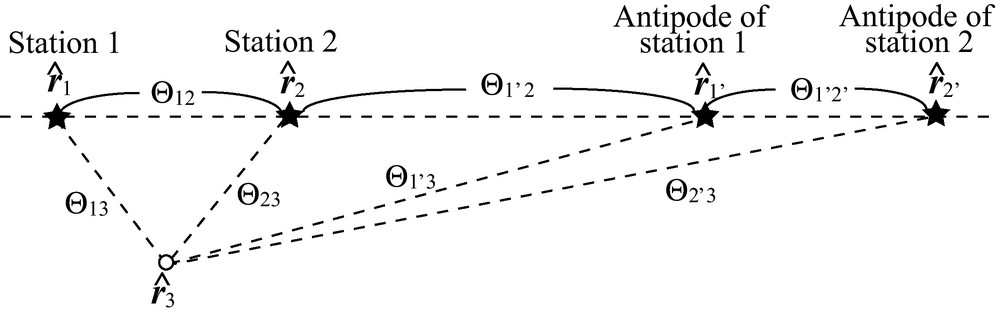
Schematic map of the geometry of stations and their antipodes. Star symbols show the locations of stations at ${\hat{r}}_{1}$ and ${\hat{r}}_{2}$ , and those of their antipodes at ${\hat{r}}_{1}^{'}$ and ${\hat{r}}_{2}^{'}$ . The open circle shows the location of a phase velocity anomaly at ${\hat{r}}_{3}$ .
Fig. 2. Carte schématique de la géométrie des stations et de leurs antipodes. Les symboles en étoile montrent la localisation des stations à ${\hat{r}}_{1}$ et ${\hat{r}}_{2}$ et celle de leurs antipodes ${\hat{r}}_{1}^{'}$ et ${\hat{r}}_{2}^{'}$ . Le cercle vide montre la localisation d’une anomalie de vitesse de phase à ${\hat{r}}_{3}$ .

5 2-D phase sensitivity kernel in a spherically symmetric Earth model for a homogeneous source distribution

To obtain a phase sensitivity kernel for phase–velocity perturbations, the causal part of an R1 or G1 wave packet $ϕ_{α}^{c, 1} ({\hat{r}}_{1}, {\hat{r}}_{2},, ω)$ is isolated as follows:

ϕ_{α}^{c, 1} ({\hat{r}}_{1}, {\hat{r}}_{2}, ω) = \frac{{\hat{Ψ}}_{α α}^{e} (ω) 2 π^{2} Q_{α} (ω) C_{α} (ω)}{ω} g_{α}^{1} (Θ_{12}, ω) e^{\frac{π}{2} i} .

(33)

The causal part of the Born sensitivity kernel is defined as follows:

K_{α}^{c, 1} = \frac{1}{2} (K_{α}^{1} - H (K_{α}^{1}) i)

, where

H

represents the Hilbert transform in the frequency domain. For simplicity, the source term

{\hat{Ψ}}_{α α}^{e}

is assumed to be a smooth function in the frequency domain. Then, perturbation of the causal part

δ ϕ_{α}^{c, 1}

can be written as

δ ϕ_{α}^{c, 1} = \int_{Σ} \frac{δ c_{α} ({\hat{r}}_{3}, ω)}{c_{α}} K_{α}^{c, 1} ({\hat{r}}_{1}, {\hat{r}}_{2}, {\hat{r}}_{3}, ω) d Σ_{3} .

(34)

The Rytov approximation is employed to obtain a phase sensitivity kernel for phase–velocity perturbations (e.g. Yoshizawa and Kennett, 2005; Zhou et al., 2004). In the Rytov method, the logarithm of the cross spectrum $ϕ_{α}^{c, 1}$ is considered instead of the wavefield itself. By taking the logarithm, $ϕ_{α}^{c, 1}$ can be divided into real (amplitude) and imaginary (phase) parts, as follows:

\ln ϕ_{α}^{c, 1} = \ln (A_{α}^{1} \exp (- ψ_{α}^{1} i)) = \ln A_{α}^{1} - ψ_{α}^{1} i,

(35)

where

A_{α}^{1}

is the amplitude of the causal wave packet, and

ψ_{α}^{1}

is its phase. The phase perturbation

δ ψ_{α}^{1}

for propagation along the minor arc (R1 or G1) is given by

δ ψ_{α}^{1} = \int K_{p, α}^{1} ({\hat{r}}_{1}, {\hat{r}}_{2}, {\hat{r}}_{3}, ω) \frac{δ c}{c} d Σ_{3},

(36)

where the phase sensitivity kernel

K_{p, α}^{1}

is the imaginary part of

- K_{α}^{c, 1} / ϕ_{α}^{c, 1}

Using the asymptotic kernel $K_{α}^{c, 1}$ , a phase sensitivity kernel for R1 or G1 can be written as

K_{p, α}^{1} = - \frac{k_{α}^{\frac{3}{2}}}{\sqrt{2 π}} {(\frac{\sin Θ_{12}}{\sin Θ_{13} \sin Θ_{23}})}^{\frac{1}{2}} \cos (k_{α} (Θ_{13} + Θ_{23} - Θ_{12}) - \frac{π}{4}) e^{- \frac{ω (Θ_{13} + Θ_{23} - Θ_{12})}{2 Q_{α} C_{α}}} .

(37)

This expression of the phase sensitivity kernel is the same as that for phase measurements of earthquake data (Yoshizawa and Kennett, 2005). The equivalence of the expressions serves as validation of ambient noise tomography. Of course, this discussion is valid only under the assumptions of one-dimensional background structure and a homogeneous source distribution.

Actual phase-velocity anomalies are measured with a finite frequency band (e.g. Bensen et al., 2007). To consider a sensitivity kernel for phase measurements, an averaged phase-velocity kernel ${\bar{K}}_{p, α}^{1}$ in a certain frequency band is better than that at a single frequency. An averaged kernel ${\bar{K}}_{p, α}^{1}$ is defined as follows:

{\bar{K}}_{p, α}^{1} = \frac{1}{Δ f} \int_{f_{0} - Δ f / 2}^{f_{0} + Δ f / 2} K_{p, α}^{1} d f,

(38)

where f₀ is the central frequency and Δf is the frequency band width.

In the same manner, a phase sensitivity kernel $K_{p, α}^{2}$ for R2 or G2 is given by

K_{p, α}^{2} = \frac{k_{α}^{\frac{3}{2}}}{\sqrt{2 π}} {(\frac{\sin Θ_{12}}{\sin Θ_{13} \sin Θ_{23}})}^{\frac{1}{2}} (\sin (k_{α} (Θ_{1^{'} 3} + Θ_{23} - Θ_{1^{'} 2}) - \frac{π}{4}) e^{- \frac{ω (Θ_{1^{'} 3} + Θ_{23} - Θ_{1^{'} 2})}{2 Q_{α} C_{α}}}

(39)

+ \sin (k_{α} (Θ_{13} + Θ_{2^{'} 3} - Θ_{1 2^{'}}) - \frac{π}{4}) e^{- \frac{ω (Θ_{13} + Θ_{2^{'} 3} - Θ_{1 2^{'}})}{2 Q_{α} C_{α}}} - \cos (k_{α} (Θ_{1^{'} 3} + Θ_{2^{'} 3} - Θ_{12}) - \frac{π}{4}) e^{- \frac{ω (Θ_{1^{'} 3} + Θ_{2^{'} 3} - Θ_{1^{'} 2^{'}})}{2 Q_{α} C_{α}}}) .

(40)

It is also possible to define an averaged phase-velocity kernel

{\bar{K}}_{p, α}^{2}

Figure 3 shows a typical example of the phase sensitivity kernels ${\bar{K}}_{p, α}^{1}$ and ${\bar{K}}_{p, α}^{2}$ at a central frequency of 7.5 mHz for a frequency band width of 5 mHz. The sensitivity is concentrated within the first Fresnel zones. The side lobes of the kernels are suppressed due to averaging in the frequency domain. The expression of the R2 kernel is equivalent to that for earthquake data (Spetzler et al., 2002), which validates its application of ambient noise tomography using the observed phase-velocity anomalies of R2 data (Nishida et al., 2009).

Fig. 3
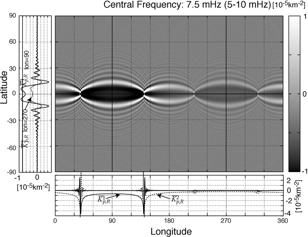
Imaginary part of the Rytov sensitivity kernels ( ${\bar{K}}_{p, α}^{1}$ and ${\bar{K}}_{p, α}^{2}$ ) of the fundamental Rayleigh wave at a central frequency of 7.5 mHz (from 5 to 10 mHz). Each station is located on the equator. The lower panel and the left-hand panel show slices of the kernels along the paths indicated by solid lines (an equatorial path, and the lines of longitude at 90° and 140°). The lower panel shows that the kernels have negative values along the minor and major arcs. Fig. 3. Partie imaginaire des noyaux de sensibilité de Rytov ( ${\bar{K}}_{p, α}^{1}$ et ${\bar{K}}_{p, α}^{2}$ ) du mode fondamental de l’onde de Rayleigh, à une fréquence centrale de 7,5 mHz (de 5 à 10 mHz). Chaque station est localisée sur l’Equateur. Le panneau inférieur et le panneau de gauche montrent des coupes des noyaux le long de trajets indiqués par des lignes continues (trajet équatorial et sur les lignes de longitude à 90° et 140°). Le panneau inférieur montre que les noyaux ont des valeurs négatives le long des arcs mineurs et majeurs.

6 Effects of heterogeneous distribution of sources on a Born sensitivity kernel

This section considers the effects of heterogeneous distribution of sources on the Born sensitivity kernel. For simplicity, the kernel $K_{α}^{1}$ is considered in a spherically symmetric case for the minor arc. It is simply assumed, phenomenologically, that the cross spectrum $ϕ_{α}^{1}$ has only azimuthal dependency, as follows:

ϕ_{α}^{1} (Δ_{12}^{1}, ω) = {\hat{Ψ}}_{α α}^{e} \frac{2 π^{2} Q_{α} C_{α}}{ω} (a (ϕ_{12}) g_{α}^{1} (Δ_{12}^{1}, ω) e^{\frac{1}{2} π i} + a (ϕ_{21}) g_{α}^{1 *} (Δ_{12}^{1}, ω) e^{- \frac{1}{2} π i}),

(41)

where a(φ) is a real coefficient that varies as a function of azimuth, and φ₁₂ is the back-azimuth to

{\hat{r}}_{2}

{\hat{r}}_{1}

. Because the focus is on the perturbation of a time-symmetric part of a CCF, the real part of the Born sensitivity kernel

K_{α}^{1}

is evaluated, as follows:

ℜ [K_{α}^{1}] \propto - {a (ϕ_{23}) + a (ϕ_{13})} \sin (k_{α} (Θ_{23} + Θ_{13})) - {a (ϕ_{23}) - a (ϕ_{13})} \cos (k_{α} (Θ_{23} - Θ_{13})),

(42)

where ℜ indicates the real part. The first term shows an elliptic pattern with foci at the stations, whereas the second term shows a hyperbolic pattern with foci at the stations. The second term vanishes in the case of a homogeneous source distribution, as in Eq. (31). If the time symmetry of the CCF is broken because of a heterogeneous source distribution, the second term would take on a hyperbolic pattern. Thus, the antisymmetry causes a bias in phase velocity maps, even without phase changes in the causal and acausal parts. Note that the second term vanishes in the case of

| {\hat{r}}_{3} | ≫ | {\hat{r}}_{2} - {\hat{r}}_{1} |

Of course, the coefficient a(φ) may have a imaginary part because an incomplete source distribution also causes a bias in the phase from 0 to π/4 (Kimman and Trampert, 2010). The imaginary part also causes a severe bias of the Born sensitivity kernel.

7 Conclusion

A theory of Born and phase sensitivity kernels was developed for a CCF using potential representation for surface waves. Simple forms were shown of Born and phase sensitivity kernels of a CCF in a spherically symmetric Earth model, assuming a homogeneous source distribution. The expression of the resultant phase sensitivity kernel is equivalent to that for phase measurements of earthquake data. This equivalence indicates the validity of ambient noise tomography under the given assumptions. The incomplete source distribution defines a hyperbolic pattern with foci at the pair of stations in a spherically symmetric case, which would generate a bias in the measured phase-velocity anomaly.

Acknowledgment

The author thanks Dr. Anne Seiminski, an anonymous reviewer, and the associate editor Dr. Michel Campillo for their constructive comments.

Bibliographie

[Bensen et al., 2007] G.D. Bensen; M.H. Ritzwoller; M.P. Barmin; A.L. Levshin; F. Lin; M.P. Moschetti; N.M. Shapiro; Y. Yang Processing seismic ambient noise data to obtain reliable broad-band surface wave dispersion measurements, Geophys. J. Int., Volume 169 (2007), pp. 1239-1260

[Bensen et al., 2009] G.D. Bensen; M.H. Ritzwoller; Y. Yang A 3D shear velocity model of the crust and uppermost mantle beneath the United States from ambient seismic noise, Geophys. J. Int., Volume 177 (2009), pp. 1177-1196

[Cupillard and Capdeville, 2010] P. Cupillard; Y. Capdeville On the amplitude of surface waves obtained by noise correlation and the capability to recover the attenuation: a numerical approach, Geophys. J. Int., Volume 181 (2010), pp. 1687-1700

[Dahlen and Tromp, 1998] F.A. Dahlen; J. Tromp Theoretical Global Seismology, Princeton University Press, NJ, USA, 1998 (1025 p)

[Dziewonski and Anderson, 1981] A.M. Dziewonski; D.L. Anderson Preliminary reference Earth model, Phys. Earth. Planet. Inter., Volume 25 (1981), pp. 97-356

[Fukao et al., 2002] Y. Fukao; K. Nishida; N. Suda; K. Nawa; N. Kobayashi A theory of the Earth’s background free oscillations, J. Geophys. Res., Volume 107 (2002) no. B9, p. 2206

[Haubrich et al., 1963] R. Haubrich; W. Munk; F. Snodgrass Comparative spectra of microseisms and swell, Bull. Seismol. Soc. Am., Volume 53 (1963), pp. 27-37

[Kimman and Trampert, 2010] W.P. Kimman; K. Trampert Approximations in seismic interferometry and their effects on surface waves, Geophys. J. Int., Volume 182 (2010), pp. 461-476

[Lin et al., 2009] F.C. Lin; M.H. Ritzwoller; R. Snieder Eikonal Tomography: Surface wave tomography by phase-front tracking across a regional broad-band seismic array, Geophys. J. Int., Volume 177 (2009), pp. 1091-1110

[Longuet-Higgens, 1950] M.S. Longuet-Higgens A theory of the origin of microseisms, Phil. Trans. Roy. Soc. London, Volume 243 (1950), pp. 1-35

[Nakahara, 2006] H. Nakahara A systematic study of theoretical relations between spatial correlation and Green’s function in 1D, 2D and 3D random scalar wave fields, Geophys. J. Int., Volume 167 (2006), pp. 1097-1105

[Nishida and Fukao, 2007] K. Nishida; Y. Fukao Source distribution of Earth’s background free oscillations, J. Geophys. Res., Volume 112 (2007), p. B06306

[Nishida et al., 2008] K. Nishida; H. Kawakatsu; K. Obara Three-dimensional crustal S-wave velocity structure in Japan using microseismic data recorded by Hi-net tiltmeters, J. Gephys. Res., Volume 113 (2008), p. B10302

[Nishida et al., 2009] K. Nishida; J.P. Montagner; H. Kawakatsu Global Surface Wave Tomography Using Seismic Hum, Science, Volume 326 (2009), p. 112

[Sanchez-Sesma and Campillo, 2006] F.J. Sanchez-Sesma; M. Campillo Retreival of the Green function from cross-correlation: the canonical elastic problem, Bull. Seismol. Soc. Am., Volume 96 (2006), pp. 1182-1191

[Shapiro et al., 2005] N. Shapiro; M. Campillo; L. Stehly; M. Ritzwoller High-Resolution Surface-Wave Tomography from Ambient Seismic Noise, Science, Volume 307 (2005), pp. 1615-1618

[Snieder, 2004] R. Snieder Extracting the Green’s function from the correlation of coda waves: A derivation based on stationary phase, Phys. Rev. E, Volume 69 (2004), p. 046610

[Spetzler et al., 2002] J. Spetzler; J. Trampert; R. Snieder The effect of scattering in surface wave tomography, Geophys. J. Int., Volume 149 (2002), pp. 755-767

[Tanimoto, 1990] T. Tanimoto Modelling curved surface wave paths; membrane surface wave synthetics, Geophys. J. Int., Volume 102 (1990), pp. 89-100

[Tarantola., 1984] A. Tarantola Inversion of seismic reflection data in the acoustic approximation, Geophysics, Volume 49 (1984), pp. 1259-1266

[Tromp and Dahlen, 1993] J. Tromp; F.A. Dahlen Variational principles for surface wave propagation on a laterally heterogeneous Earth–III, Potential representation, Geophys. I. Int., Volume 112 (1993), pp. 195-209

[Tromp et al., 2010] J. Tromp; Y. Luo; S. Hanasoge; D. Peter Noise cross-correlation sensitivity kernels, Geophys. J. Int., Volume 183 (2010), pp. 791-819

[Yoshizawa and Kennett, 2005] K. Yoshizawa; B.L.N. Kennett Sensitivity kernels for finite-frequency surface waves, Geophys. J. Int., Volume 162 (2005), pp. 910-926

[Zhou et al., 2004] Y. Zhou; F.A. Dahlen; G. Nolet Three-dimensional sensitivity kernels for surface wave observables, Geophys. J. Int., Volume 158 (2004), pp. 142-168

Commentaires - Politique

Ces articles pourraient vous intéresser

Intrinsic versus extrinsic seismic anisotropy: Surface wave phase velocity inversion

Nian Wang; Jean-Paul Montagner; Gäel Burgos; ...

C. R. Géos (2015)

Ambient noise tomography with a large seismic array

Michael H. Ritzwoller; Fan-Chi Lin; Weisen Shen

C. R. Géos (2011)

Nouveaux développements de l’imagerie et du suivi temporel à partir du bruit sismique

Michel Campillo; Haruo Sato; Nikolai M. Shapiro; ...

C. R. Géos (2011)