

1 Introduction
Lake Pavin is located in the volcanic chain of France's Auvergne region. It is qualified as a crater lake, circular in shape with a depth of 92 m and a surface area of 0.44 km2. Located southeast of the Mont-Dore range and 4 km southwest of the town of Besse and Saint-Anastaise, this lake exhibits the particularity of a meromixis condition. Only the mixolimnion (from 0 to 60 m) is affected by seasonal overturns, as opposed to the monimolimnion (layer in the 60–92 m depth range) (Martin, 1985).
The monimolimnion is characterized by steep gradients of dissolved matter, dissolved gases (especially CH4 and CO2) and by complete and permanent anoxia (Michard et al., 1994). The lake bottom is exposed to a heat flux of geothermal origin; the water temperature of the monimolimnion exceeds by about 1 °C that of the lower part of the mixolimnion. Moreover, the concentration of dissolved salts in the monimolimnion is substantially greater than the concentration found in the mixolimnion (the specific conductivity at 25 °C between these two compartments varies from 50 to nearly 500 μS cm−1), thus ensuring monimolimnion stability. The heat and dissolved compounds of the monimolimnion actually diffuse in the direction of the mixolimnion. From one year to the next, the position and intensity of temperature gradient and dissolved species gradient (chemocline) may vary slightly, depending on mixing variability in the mixolimnion. This variability seems to be closely linked to the intensity of winter mixing and ice cover. In 2006 for example, a diffusive front could be observed at depths reaching 30 m. The combined diffusion of matter and heat from the monimolimnion, although relatively weak, ensures the stability of the water column below depths of 30 m. (Assayag et al., 2008). Therefore, the detection depth of increasing temperature and conductivity gradients varies from one year to another, the steepness of the gradients may vary too but the meromictic characteristics remain.
More generally, understanding meromixis and the factors that lead to this particular state is a major challenge at present because many inland water bodies are moving towards meromixis in the current context of climate change and increasing anthropogenic inputs of nutrients (Hakala, 2004). Moreover, the sudden instability of meromictic lakes can lead to disasters by massive carbon dioxide and methane discharge into the atmosphere. A lethal eruption of Lake Nyos happened in 1986 in Cameroon and the exact cause of this eruption is still discussed today (Touret et al., 2010).
Both the origins and mechanisms involved in the stability of the Lake Pavin meromixis are poorly known. The origin may in fact be: (i) ectogenic (in the case of a low-salinity water inflow into the mixolimnion); (ii) crenogenic (inflow of highly-saline water into the monimolimnion due to volcanic activity); or (iii) biogenic (biological activity increases dissolved matter concentration on the lake bottom) (Hutchinson, 1957). As regards Lake Pavin, each of these three individual origins could play a role: (i) a low-salinity spring in the mixolimnion may stabilize the interface between mixo- and monimolimnion by increasing the salinity gradient; (ii) a mineral spring in the monimolimnion may similarly strengthen the gradient at the interface; (iii) and biological activity may also increase the particle content, and therefore the density, in the monimolimnion. One of the most common hypotheses (Aeschbach-Hertig et al., 2002; Assayag et al., 2008; Michard et al., 1994) relates to the presence of one or several sublacustrine springs that would contribute to conserve gradients at the mixolimnion–monimolimnion interface. The existence of such springs is supported by the water balance, which fails to achieve equilibrium when only the water inflow via the catchment basin is taken into account.
Many contributions to the study of the hydrological processes occurring in Lake Pavin have been proposed over the last thirty years, most of them being based on geochemical methods (Aeschbach-Hertig et al., 2002; Assayag et al., 2008; Martin, 1985; Meybeck et al., 1975) The various estimates tend to converge on a sublacustrine water inflow on the order of 20 L/s as an annual average (Assayag et al., 2008) of which approximately 2 L/s would be injected at the bottom of the monimolimnion by means of a mineral spring with the remainder arriving in the mixolimnion (Aeschbach-Hertig et al., 2002)
It is proposed here, on the basis of some strictly physical measurements carried out during 2006 and 2007, to examine the hypothesis of the existence of a spring flowing into the Lake Pavin mixolimnion, at a depth of around 50 m. We will seek to characterize and understand the role of this spring in the conservation of the lake meromixis. A modelling approach was developed to enable us to compare the flux of matter transferred from the monimolimnion towards the mixolimnion in two scenarios: absence or presence of a spring. This article examines the temporal variability of this flux, based on the observations from 2006 and 2007. Moreover, the role of the spring in controlling mixing depth during winter convection is studied.
The presence of a mineralized spring within the monimolimnion was first predicted as long ago as 1975 as an explanation of the observed gradients at the mixo–monimolimnion interface (Meybeck et al., 1975). Ten years later, Martin (1985) used a box model to explain both the hydrologic balance and tritium measurements by continuing to conjecture that a unique spring existed within the monimolimnion. In 2007, Assayag et al. (2008) tested various scenarios by applying the 1D AQUASIM model (Reichert, 1994), which incorporates, in particular, the hypothesis of a sublacustrine spring within the mixolimnion, complemented by a very slight vertical diffusivity between monimolimnion and mixolimnion, as an explanation of recorded Δ18O anomalies. This hypothesis was corroborated by the observation of a cold temperature anomaly on the vertical profiles measured with a multiparameter (conductivity-temperature-depth) probe in September 1996, which was not apparent on the September 1994 profiles (Aeschbach-Hertig et al., 2002). This approximately −0.06 °C anomaly was noticed at depths of between 45 and 50 m. The authors also identified a slight drop in dissolved oxygen at these same depths, with no recorded conductivity anomaly.
More recently, the presence of water inflow has been confirmed (Assayag et al., 2008), based on isotopic analyses of the 18O concentration from a series of extractions conducted between 2002 and 2004 over the entire water column. A precise flow rate evaluation from another spring in the monimolimnion at 1.7 L/s, along with the corresponding hydrologic balance, leads to a flow rate close to 18 L/s in the mixolimnion.
2 Materials and methods
Thermal microstructure profiles were done using a device called SCAMP (for Self-Contained Autonomous Micro-Profiler, PME Inc., USA) at a monthly pace between May 2006 and June 2007. The SCAMP accuracy was 0.005 °C for temperature measurements with a resolution of 0.0005 °C. The resolution of conductivity measurement reached 0.2 μS cm−1 with an absolute accuracy of 3 μS cm−1. SCAMP served the purpose of solving the thermal microstructure at a millimetre scale inside the water column, even though in this instance the device was being used as a CTD probe. The profiles shown were carried out at the centre of the lake.
Continuous temperature measurements were recorded from July 2006 to July 2007 with a LDS (Lake Diagnostic Station, PME Inc., USA), except for the winter period when the lake froze. The data acquisition time step was set at 30 s, and temperature sensors were accurate to within 0.001 °C with a resolution of 0.0005 °C. A temperature-chain of LDS was buoyant and allowed tracking temperature variations between 4 and 70 m depth. (with sensors positioned at depths of 4, 7, 15, 25, 35, 45, 50, 53, 56, 58, 60 and 70 m). These sensors were placed so as to increase observation density within steep gradient zones. Changes in lake level are very small (about 30 cm) and were measured by an OTT probe.
During the winter period, Starmon-mini thermometers (Star-Oddi, Iceland) were installed on a buoyant chain at depths comparable to those of the LDS thermometers (i.e. at depths varying between 4 and 70 m). The data acquisition time step remained at 30 s with these measurements, yet accuracy dropped to 0.01 °C and resolution to 0.005 °C.
Between April 26 and June 26, 2007, two Aanderaa oxygen 3830 optodes (Aanderaa Data Instruments, Norway) were introduced in order to continuously monitor the dissolved oxygen concentration at fixed depths within the oxycline (at both 51 and 56 m). A 30-min acquisition time step was adopted for these sensors. The measurement range extends from 0 to 500 μmol/l of dissolved oxygen, with a resolution of less than 1 μmol/l and a relative precision below 5% (< 8 μmol/l). The response stabilization time (t90) was 3 min. Over the target measurement interval, calibration controls reveal that the level of sensor drift remains lower than 5% during a three-month period.
The mini-Starmon thermal line and optodes were positioned close to the centre of the lake, whereas the LDS was located 150 m east of this point in order to analyse the internal wave field in Lake Pavin, which will be the purpose of a further publication.
2.1 Modelling tool
Solute transport is modelled by a diffusion equation, whereas the presence of density instabilities is modelled through homogenizing the unstable zone.
The vertical diffusion of a passive tracer at concentration C in the water column follows the one-dimensional equation:
| (1) |
Diapycnal diffusivity (which means diffusion through layers of the same density) is calculated by employing the method described below. The mass density of water is deduced from temperature and salinity, which was recalculated from conductivity at 25 °C (Aeschbach-Hertig et al., 2002). The Brunt-Väisälä frequency (N) is the frequency at which a vertically displaced parcel oscillates within a statically stable environment (gravity wave). The squared Brunt-Väisälä frequency (N2) equals:
| (2) |
In the vicinity of the mixolimnion–monimolimnion interface, i.e. at depths between 55 and 60 m, the salinity guarantees the water column stability by countering the thermal gradient due to heating by the geothermal flux. N2 varies from 10−4 s−2 at the chemocline to 10−8 in the hypolimnetic part of the mixolimnion (depending on the size of the box used to average temperature and salinity gradients and on the inter- and intra-annual variability). Values of N2 calculated for two independent surveys in 2006 and 2007 are shown in Fig. 1. The interannual variability of stratification in the mixolimnion appears to be very high.
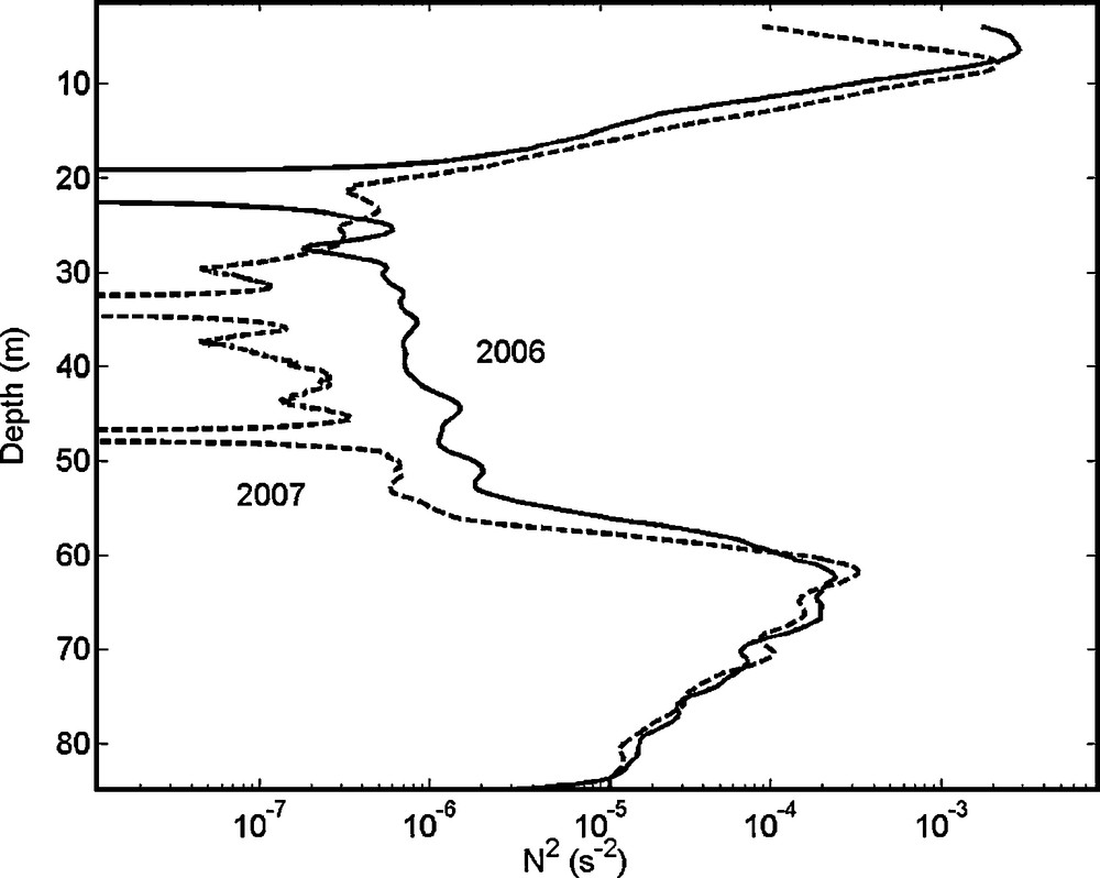
Squared Brunt-Vaisala frequency (s−2) calculated from 2 m box sliding averaged SCAMP profiles in April 2006 (thick line) and April 2007 (dotted line).
Fréquence de Brunt-Vaisala élevée au carré (s−2), calculée à partir de moyenne glissante sur 2 m des profils de conductivité et de température du SCAMP acquis en avril 2006 (ligne épaisse) et avril 2007 (ligne pointillée).
If Eq. (2) gives a positive result, the vertical turbulent diffusion coefficient can be calculated with Osborn's Law (1980):
| (3) |
In the case where the right member of Eq. (2) is negative or exceeds a threshold corresponding to that of convective instability (i.e. Kz > 10−2 m2·s−1), the tracer content of the water layers is homogenized respecting mass conservation. In 2007, this threshold was exceeded at several depths in the water column.
In the model, the heat and solute diffusion coefficients are assumed to be equal. In fact, Kz values in the mixolimnion imply that turbulence is the main phenomenon that leads to mass and heat transport. Close to the chemocline, Kz values are close to heat and molecular diffusivity (sometimes even below heat diffusivity). Differences in diffusivity of solute and heat are supposed to lead to detectable double-diffusive staircases in the density profiles, when the turbulent diffusivity is very low. These staircases are the result of mixing zones (isodensity) alternating with stratified zones. The calculation of the ratio between saline and temperature contributions to density confirms the possibility to observe double diffusive staircases close to the chemocline. Moreover, winter mixing increases turbulent mixing close to the chemocline and prevents the development of staircases. Equation (1) is then solved by implementing a finite differences method with Δz = 25 cm and Δt = 0.3 days. The sublacustrine spring flow modifies the temperature and conductivity gradients; therefore the diapycnal diffusivity coefficient needs to be calculated at each time step.
The assumptions on the initial conditions and boundary conditions are presented together with the simulation results, because the observations determined the values of input parameters for the model.
3 Results
3.1 Detection of temperature drops propagating upwards within the mixolimnion
Temperature drops on the profiles were observed several times during 2007, while no such drops could be detected on profiles acquired throughout 2006. Detection of cooling events varies from one year to another confirming previous observations (Aeschbach-Hertig et al., 2002). Drops are combined with mixing phenomena, as reflected by locally fluctuating temperature measurements between 40 and 50 m (on the profile dated June 27, 2007). Fig. 2 shows the appearance of cold thermal drops on the SCAMP profiles for May and June 2007. Thermal drops of lower amplitude were also detected also in April 2007 which may be attributed to the same external cause. As April water temperatures are lower than those in May water temperature in the mixolimnion, these drops are less pronounced. The anomalies range between 40 and 55 m and may reach 0.05 °C. At this stage, two hypotheses can be formulated: either the injection of cold water could not be detected in April 2007 as the temperature of the anomaly is similar to the mixolimnion one at this time of year, or there is no anomaly at all, meaning that such inflow is occurring intermittently at these depths.
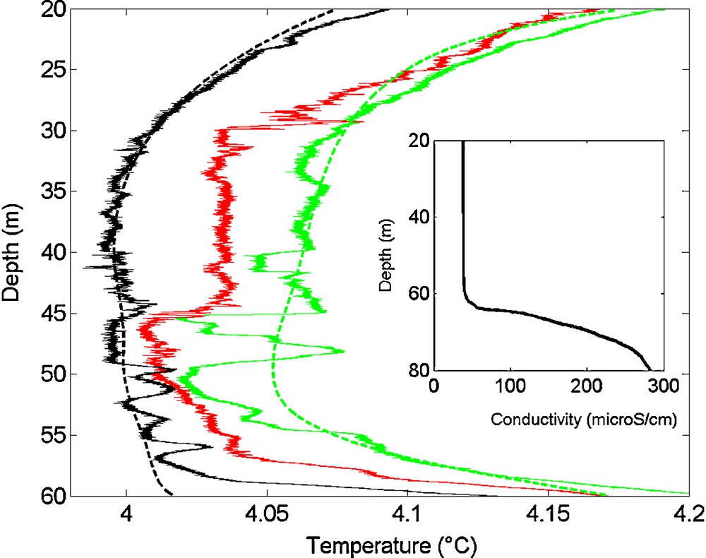
Temperature profiles between 20 and 60 m generated with SCAMP on April 25, 2007 (shown in black), May 31, 2007 (red) and June 27, 2007 (green). The conductivity profile of April 2007 between 20 and 80 m depth lies in the right inserted box.
Profils de température entre 20 et 60 m réalisés avec le SCAMP le 25/04/2007 (en noir), le 31/05/2007 (en rouge) et le 27/06/2007 (en vert). Le profil de conductivité d’avril 2007 figure dans l’encadré à droite.
The temperature “anomaly” was estimated by ascribing the deviation on a calculated theoretically “simply-diffusive” temperature profile between monimolimnion and mixolimnion. In April 2007, the temperature “anomaly” was estimated by ascribing the deviation to a large scale sliding averaged temperature profile (Fig. 2). For the following months, the April “simply diffusive” profile was modified by linearly modifying temperature boundary conditions between April and June 2007 (at 30 and 70 m) and applying the heat diffusion equation to the temperature using Kz calculated from Osborn's formula (see Materials and methods). Even if the deviation from the “simply-diffusive profile” cumulates different external influences (especially in April 2007), it is one method of quantifying the perturbation. This drop was −0.027 °C at 46 m at the end of May 2007 and −0.056 °C at 50 m one month later. It is worthwhile to note that no conductivity anomaly was detected by SCAMP recordings at the centre of the lake. The electrochemical composition of this water inflow thus approximates the mixolimnion composition.
In addition, the LDS temperature analysis between April 25 and July 19, 2007 (Fig. 3A) indicates a bottom-to-top propagation in the water column of a colder water flow, detectable from the 53 m sensor and capable of propagating intermittently and extending to the 25 m sensor. Three major temperature drops are also highlighted (May 14–16, 2007, June 12–20, 2007 and July 11–13, 2007) throughout the period. The beginning and end time of the cooling events are determined through different processing steps. First, the sliding mean of the time series is computed at a large time-scale (10 days) to obtain the trend (T)–see Fig. 3A. Second a sliding mean (called SLIM) is calculated at a small time-scale (with a 1 hour window) to remove the effects of small-scale turbulence. If the difference between the trend (T) and the sliding mean (SLIM) exceeds twice of the standard deviation σ, then it is the starting point of a cooling event. When the SLIM reaches the general trend T, it is the end date of the event. Vertical velocities related to the motion of the parcel of water are computed using the different beginning time of the cooling events at the different depths.
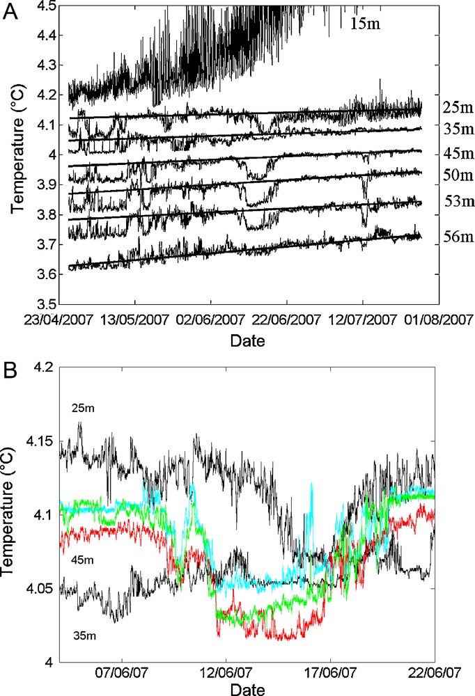
A. Temperature time series at depths ranging between 15 and 56 m over the period April 23–August 1, 2007. To improve visualization, an offset was incorporated into some recordings: T_15m = no offset, T_25m = no offset, T_35m = no offset, T_45m = −0.1 °C, T_50m = −0.2 °C, T_53m = −0.3 °C, T_56m = −0.4 °C. Bottom-to-top propagating events are represented by straight lines. B. Close-ups on the second major temperature cooling event without offset. Black: 25 and/or 35 m, red: 45 m, teal: 50 m, green: 53 m.
A. Série temporelle des enregistrements de température entre 15 et 56 m et entre le 23/04/07 et le 01/08/07. Pour une meilleure visualisation, certains enregistrements ont subi un offset : T_15m = pas d’offset, T_25 = pas d’offset, T_35m = pas d’offset, T_45m = −0,1 °C, T_50m = −0,2 °C, T_53m = −0,3 °C, T_56m = −0,4 °C. Les événements se propageant du bas vers le haut sont matérialisés par des lignes droites. B. Zooms sur le deuxième évènement majeur de refroidissement des températures sans offset. Noir : 25 et/ou 35 m, Rouge : 45 m. Cyan : 50 m, Vert : 53 m. Masquer
A. Série temporelle des enregistrements de température entre 15 et 56 m et entre le 23/04/07 et le 01/08/07. Pour une meilleure visualisation, certains enregistrements ont subi un offset : T_15m = pas d’offset, T_25 = pas d’offset, T_35m = pas d’offset, T_45m = −0,1 °C, Lire la suite
These events represent thermal drops that nearly reach −0.1 °C, the first two of which generate an impact to a depth of 25 m. The most significant temperature decreases were recorded on thermometers placed 50 and 53 m, with a time-lag indicating the bottom-to-top cold water mass propagation.
Fig. 3B shows the second event occurring between June 12 and 20, 2007. Based on these observations, we are in a position to calculate the apparent velocity of the rise of the thermal anomaly within the water column for this particular event. The apparent velocity is calculated by considering the time-lag between the detection of cooling at two different depths. Between 53 and 45 m, this velocity equals 5.7 × 10⁻⁴ m·s−1, whereas between 45 and 25 m, it drops to 2.9 × 10⁻⁴ ms−1. During the third event (July 11–13, 2007), the cold anomaly lasts for a shorter length of time and only extends to a depth of 45 m.
For both of these events, the temperature at 35 m, which represents the minimum profile value, does not exhibit any significant variation as the water mass passes by. This water mass displacement may be ascribed either to an advective effect related to the sublacustrine spring kinetic energy or to a convective effect related to a density difference.
3.2 Distinction between thermal drops and turbulence effect
The duration of these cooling cycles serves to distinguish between local mixing phenomena and “overturns” that often appear in slightly-stratified hypolimnions of freshwater lakes. In this case, the resulting temperature variations would affect the water column over a height on the order of a few meters and would last up to several hours. The length T of a static or convective or shear instability event within a stratified medium is inversely proportional to the Brunt-Väisälä frequency, which lies in the range of 10−3·s−1 in the Lake Pavin mixolimnion (Assayag et al., 2008). The period of an instability can be approximated by: T ≈ 24 N−1 (Thorpe and Jiang, 1998), i.e. at most about 6 hours in the lower part of the mixolimnion. Since these events were observed over several days, it may be deduced that local instabilities are not the cause of the recorded thermal anomalies.
The sudden temperature drops noticed in the mixolimnion cannot be ascribed to heat fluxes on the lake surface or bottom given that temperature recordings below the thermocline (at 25 m) or above the chemocline (at 58 m) do not reveal any temperature variation. This layer of the lake is thus behaving like an isolated system, at the episode scale and at both its upper and lower boundaries, between 25 and 58 m. The temperature decreases recorded in the water column between these two depths during the studied periods indicate the necessary presence of a cold-water inflow originating from outside the system. Moreover, the minimum temperatures reached during these temperature drops were not recorded elsewhere in the water column and cannot be correlated with internal waves that would have caused intrusions at these depths. The sole hypothesis that could actually be envisaged therefore entails a sublacustrine spring.
3.3 Characterization of the spring temperature
The three cooling events correspond to temperature variations around a mean of −0.05 °C, which on average require half a day to form (Fig. 3B). The heating and cooling dissymmetry in the first event deserves our attention, as it demonstrates that cooling is caused by a sudden inflow of cold water whereas heating occurs gradually (Fig. 3B).
An evaluation of the daily heat flux was made between 50 and 55 m, i.e. in the zone of highest recorded temperature variations:
| (4) |
According to the bathymetry established by Delebecque in 1898, the volume of water between 50 and 55 m is 106 m3.
On the first event (Fig. 3B), a temperature drop of 0.07 °C was noticed in one single day. This observation over such a short time enables us to eliminate convective transfers towards the upper levels which occur with a time lag. Accordingly, we have estimated that the spring has a thermal impact of the same magnitude, between 50 and 55 m, over approximately 1/6 of the lake surface. This estimate of the horizontal plume extent was derived from spatial information collected a few years ago during a field campaign of thermal anomaly detection (Assayag et al., 2008). Equation (4) then leads to:
| (5) |
The variation in heat quantity may be ascribed to the cold spring, which has an annual average flow rate, estimated by various methods, at 20 L/s (Aeschbach-Hertig et al., 2002; Assayag et al., 2008), i.e. 1700 m3 per day. The intermittent nature of the observed cooling events reflects the intermittence of the sublacustrine spring. A number of flow rate hypotheses were tested; temperature deviations between the spring and the mixolimnion vary depending on the selected hypothesis from 2.72 °C for a flow rate of 50 L/s, 1.36 °C for a flow rate of 100L/s to 0.68 °C for a 200 L/s flow rate.
Instantaneous flow rates in excess of 200 L/s are not very realistic since they would lead to greater turbulence and high horizontal velocities in the lake.
Finally, an instantaneous flow rate of 100 L/s was selected for the following modelling approach due to its compatibility with both the heat balance and realistic spring temperatures.
In the vicinity of Lake Pavin, the hole “Creux du Soucy”, located at about 2 km from the lake, is a good candidate to explain cool water entries in the lake. The surface water inside the hole has an altitude of 1275 m (25 m higher than the elevation of the lake). The water temperature and conductivity were measured in July 2007 and were respectively 2.1 °C and 23 μS/cm (conductivity at 25 °C is 40 μS/cm). Old legends report that this hole may be directly connected to Lake Pavin by a kind of siphon (Bakalowicz, 1971). This assumption is confirmed by recent diving explorations of the hole, which showed that the hole is connected to a 50 m long quasi-vertical tunnel. The presence of fractured rocks may explain why the tunnel behaves like a siphon. Therefore, the low conductivity of Creux de Soucy water and its location are consistent with the assumption of a sublacustrine input of this water into Lake Pavin. Moreover, the temperatures of surface springs falling into Lake Pavin lie above 5 °C, far above the temperature of the entering water.
3.4 Dissolved oxygen content of the sublacustrine spring
The general annual trend in oxygen concentration within the Lake Pavin oxycline, outside of the icy period, is to decrease with time at a given depth (LGE data for years 2006 and 2007). This decrease is explained in particular by the oxidation of various dissolved compounds, such as reduced iron and manganese, in addition to ammonium and methane diffusing slowly from the mixolimnion–monimolimnion interface, consuming oxygen once its concentration begins to increase in the mixolimnion, and precipitating. Precipitates increase the particle content: a rise in particle concentration was observed by means of Doppler acoustic measurements (LADCP). Metal oxides are formed at different oxygen concentration levels, therefore at different depths, which results in observable independent layers with higher particle concentrations between 50 and 60 m (data not provided).
In 2007, periods of oxygen recharge reaching 50 μmol/l were observed at 56 m, even though no known biogeochemical mechanism is able to offer any explanation. This phenomenon was not noticed in 2006.
Fig. 4 A, B shows that these oxygen recharge periods coincide with temperature drops detected between 45 and 56 m. From May 14 to 16, 2007, oxygen recharge appeared to lag behind the cold thermal anomaly. For the second period, June 12–20, 2007, the increase in oxygen also coincided with a slight time lag compared to the temperature anomaly, which might be attributed to anomaly propagation time between temperature and oxygen sensors spaced 150 m apart horizontally. Even if the velocity of anomaly displacement lies on the order of 10−3 ms−1 and is consistent with the effect of horizontal turbulent diffusion that can be estimated at 1.5 × 10⁻¹ m2s−1 from the dimensions of Lake Pavin (Stevens et al., 2004), these measurements might also reflect the spatial (horizontal) intermittency or inhomogeneity of the spring water distribution in the hypolimnion. A temperature sensor located close to the oxygen sensor would have been useful to definitely conclude on a correlation between water drop and oxygen recharge events.
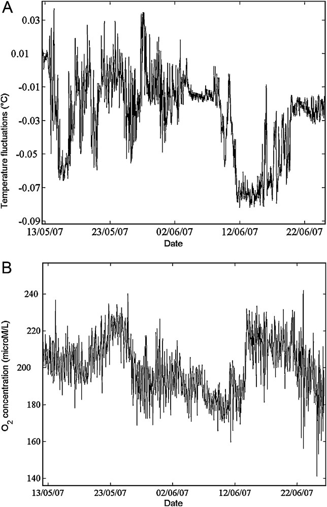
A. Temperature fluctuation around the 4 days – sliding average (in °C) at 53 m. B. Oxygen time series (in μmol/l) at a depth of 56 m.
A. Fluctuations de température autour de la moyenne glissante sur 4 jours (en °C) à 53 m. B. Séries temporelles d’oxygène (en μmol/l) à 56 m.
At a depth of 56 m, the oxygen recharge periods correspond to oxygen concentration increases of between 40 and 50 μM for an average value of 200 μM at 56 m. The other optode positioned at a depth of 50 m deep displays coincidental yet smaller fluctuations, amounting to 15 μM for an average value of 245 μM over the study period. The sensor at 56 m would thus seem to lie closer to the spring inflow depth.
3.5 Key processes involved in upward motion
Three processes may be involved in explaining temperature evolution: turbulent diapycnal diffusion, the initial kinetic energy of the spring (advection), and buoyancy (convection). Based on the velocity of the thermal anomaly rise in the water column, the first and the third hypotheses can be rejected.
For a vertical diffusion Kz equal to 10−4 m2s−1 (a high value for the Lake Pavin hypolimnion) (Assayag et al., 2008; Bonhomme et al., in prep), the layer thickness influenced by cooling specific to the spring may be estimated by:
We can now compare the advective with the convective hypothesis. The horizontal plume velocity is supposed to be much higher than the vertical plume motion. According to this hypothesis, the homogenisation is very rapid in the horizontal dimension compared with the vertical one and the study of horizontal and vertical motions can be decoupled. After the maximum spatial extent of the plume is reached, the horizontal velocity is no longer taken into account. The situation is simplified in the following way: the maximum spatial extent of the plume is assimilated to a cylindrical jet, whose diameter is the horizontal distance at which temperature differences are detectable. The injection of a fluid is supposed to occur at the lowest depth at which the temperature anomaly is detectable (55 m) and its initial vertical injection velocity is accordingly seen as the lowest vertical measurable velocity of cooling event propagation. On the vertical near the point of fluid ejection, the kinetic effect dominates the transport effect. Floatability becomes dominant beyond a characteristic distance lm, which is the ratio of movement quantity (M0) to floatability (Q0) (Eq. (6)) (Fischer et al., 1979):
| (6) |
In considering a plume of circular cross-section, M0 is defined as:
Since no salinity difference with respect to the spring can be measured, Δb0 is to be determined using Morton's formula (Eq. (7)) (Morton et al., 1956), by which one can calculate Δb0 from remote measurements.
| (7) |
Velocity w was estimated by setting a high value for the velocity of rising thermal drops observed on the LDS recordings, without any prior knowledge of the precise plume center location: w ∼ 5 × 10⁻⁴ m·s−1. This value has to be linked to measured w (see section 3.1). By using a high estimate of the flow rate q ∼ 20 Ls−1 (which is the most likely hypothesis according to (Aeschbach-Hertig et al., 2002)), an entrainment coefficient α equal to 0.1 (usual value in the case of a plume), a plume height H ∼ 25 m (as the plume rises about 25 m in the water column), a value of Δb0 ∼ 2.3 × 10⁻⁹ m4s−3 is obtained.
Application of the definition of M0 with D ∼ 150 m (because the influence of the plume is detectable within a radius of 150 m - see section 3.4), w0 ∼ 5 × 10⁻⁴ m/s and Δb0 ∼ 2.3 × 10⁻⁹ m4s−3 yields a value of lm ∼ 0.3 m. The accurate estimate of D is not of great importance since the calculation of lm is not very sensitive to D. This very low value means that floatability dominates vertical displacement in the water column after the first meter.
Note that such a low value for Δb0 is consistent with non-measurable salinity anomalies correlated with the Lake Pavin mixolimnion spring, since:
| (8) |
The following values of a0, b0 and β (a0 = 0.601, b0 = 8.45 × 10⁻⁴ and βs = 0.778 × 10⁻³) were extracted from (Aeschbach-Hertig et al., 2002). Expected conductivity differences are thus on the order of 10−2 μS/cm, making them non-measurable, which is consistent with observations.
3.6 Modelling the sublacustrine spring impact on maintaining meromixis at the intra-annual time scale
Only the convective transport hypothesis can be used to explain the observed anomaly propagation. The objective here is to focus on the impacts of the sublacustrine spring on mass transfer at the mixolimnion–monimolimnion interface. The modelling tool described above was used to investigate the role of the sublacustrine spring role in maintaining meromixis.
Changes at the mixolimnion–monimolimnion interface were simulated over a 300-day period, which corresponds to the mean unfrozen period on Lake Pavin, in two scenarios:
- • the absence of any spring;
- • the presence of a sublacustrine spring, represented by temperature and conductivity intermittently forced to their initial values on the water column between 45 and 55 m. A consequence of this forcing is to reduce the temperature and conductivity at these depths by countering the diffusive tendency of the monimolimnion towards the mixolimnion.
The initial temperature and conductivity profiles were taken from SCAMP measurements recorded on April 4, 2007. The modelled zone lies between depths of 30 and 80 m. At the boundaries of this zone, the conductivity and temperature readings are forced to their initial values at each time step.
Fluxes at the mixo–monimolimnion interface in the direction of the mixolimnion were evaluated from calculated concentration variations of a fictitious independent passive tracer, with a profile analogous to that of the conductivity and varying between 0 and 1. This independent passive tracer is only transported, does not react with any other tracer in the environment and its concentration does not influence the water density. Matter transfer was determined by calculating variations in the area delimited by the profile between 30 and 60 m, while still incorporating matter losses at zone boundaries.
Heat and dissolved matter both diffuse in the monimolimnion-to-mixolimnion direction. In turn, this diffusion changes Kz. In the scenario of no contribution from sublacustrine water around a 50-m depth, the decrease in heat and salinity gradients through diffusion causes a stability decline at the interface. The presence of water inflow able to maintain a low conductivity near the interface raises the interface stability, while stimulating mixing with the remainder of the mixolimnion shallower than 50 m. This additional water therefore helps insulate the mixolimnion from the monimolimnion by reducing vertical diffusion near the interface. Fig. 5 shows the evolution of a passive tracer concentration after 300 days of simulation in the absence or presence of the spring. The presence of the spring seems to play an important role in the mass transfer between the two compartments of the lake.
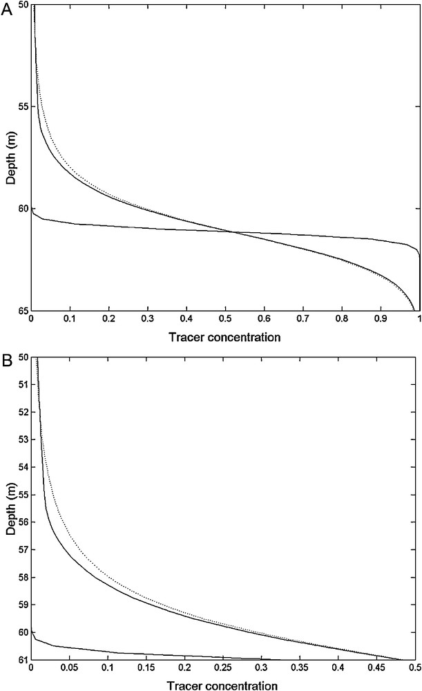
A. Evolution of the passive tracer concentration between 50 and 60 m after 300 days of simulation: Initial profile (solid line), with spring after 300 days of simulation (dashed line), and without any spring after 300 days of simulation (dotted line). B. Zoom of Fig. 5A between 50 and 61 m.
A. Évolution de la concentration en traceur passif entre 50 et 60 m après 300 jours de simulation : profil initial (trait plein), avec source après 300 jours de simulation (trait pointillé), sans source après 300 jours de simulation (petits points). B. Zoom de la Fig. 5A entre 50 et 61 m.
The flux evaluation performed with a passive tracer over a one-year period is summarized in Table 1. The presence of a spring would thus help reduce fluxes between the monimo- and mixolimnion by some 20%, with this effect tending to become more pronounced over time. This flux decrease proves significant at the annual scale and serves to limit diffusion above the monimolimnion. On the other hand, the absence of a spring causes a gradual stability decline by diffusion.
Simulation du flux de traceur en présence et en absence de la source au-dessus du monimolimnion.
| 1-year simulation | |||
| No spring | With a spring | ||
| Initial tracer mass between 30 and 80 m | 59.04 | 55.69 | 56.38 |
| Initial tracer mass between 30 and 60 m | 0.67 | 3.35 | 2.66 |
3.7 Role of the spring in maintaining meromixis at the inter-annual scale
The 2005–2006 winter was especially harsh and snowy, accompanied by a very long freezing-over of the lake. Minimum temperatures in the water column during 2006 remained below Tmd (the maximum density temperature) calculated (Eklund, 1965) at a depth of 25 m from April to September 2006. In Fig. 6, no thermal anomaly is detected between 50 and 55 m in 2006. Moreover, a comparison of thermal and conductivity profiles between 2006 and 2007 (Fig. 6) indicates that the mixolimnion bottom in 2006 exhibited a higher temperature in 2007. Moreover, the hypolimnion was more stratified in 2006. Observation of LDS data over the months of July and August 2006 confirms this finding (Fig. 7). In comparison with Fig. 3, no element reveals the presence of sublacustrine water intrusion or rising motions at a depth of 50 m during all of 2006 near the lake centre. The sublacustrine spring may have been absent (or had a very low flow) in 2006 or the position of the LDS at the lake center may not have detected the thermal impact of the spring. For example, if the density difference of the spring with mixolimnion environment is stronger in 2006 than in 2007, the rising plume moved faster up the water column. In this case, the minimum observed temperature at a depth of around 30 m throughout all of 2006 might be due to the horizontal plume extension.
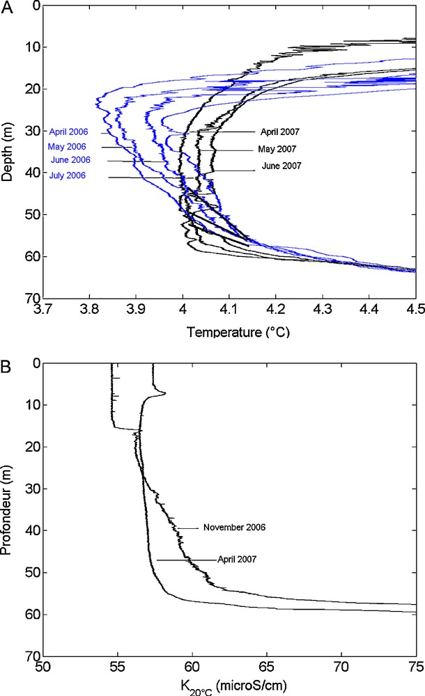
Comparison of the evolution of temperature profiles (in °C) between 2006 (blue) and 2007 (black). Each profile is separated from the next by 1 or 2 months.
Comparaison de l’évolution des profils de température (°C) entre l’année 2006 (bleu) et 2007 (noir). Chaque profil est séparé du suivant par 1 ou 2 mois.
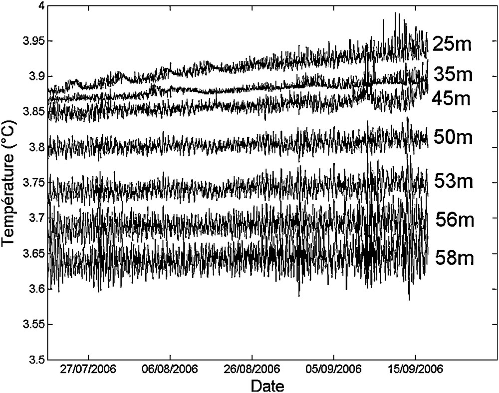
LDS temperature time series (in °C) over the period July 25–September 2, 2006 between 25 and 58 m.
Enregistrement de température du LDS (en °C) du 25/07/06 au 02/09/06 entre 25 et 58 m.
During 2007, the mixolimnion was much more homogeneous. The spring periodically added a sizable volume of low-conductivity water. In assuming overflows comparable to what has been estimated in this study, the spring contributed a volume of 4300 m3 in half a day, which is equivalent to nearly 0.1% of the volume existing from the lake bottom to around 60 m.
A seasonal overturn was observed during the 2006–2007 winter thanks to a chain of thermistors in place all winter long underneath the ice. The seasonal overturn of the lake mixolimnion occurred in two stages: in the initial stage, water adjacent to the density maximum at these depths (3.9 °C) (Eklund, 1965) dipped at the end of January to a depth in the range of 50 m. The 10 m layer above the chemocline (between 50 and 60 m) was therefore not mixed (Fig. 8). An inverse stratification then occurred between the surface and 50 m from the bottom in the mixolimnion (data not provided).
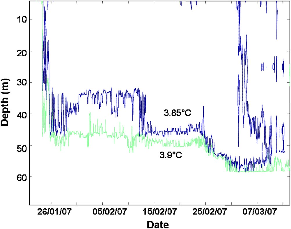
Observation of isotherms dipping between January 25 and March 10, 2007, until a depth of 58 m. Only those isotherms in the vicinity of the maximum density temperature are shown.
Observation de la plongée des isothermes du 25/01/07 au 10/03/07 jusqu’à 58 m de profondeur. Seules les isothermes voisines de la température de maximum de densité sont représentées.
The sudden inflow of a large quantity of low-salinity water around February 25, 2007 (Fig. 8) eventually flattened the salinity gradient, which enabled the seasonal overturn to touch the chemocline (at 60 m) during a second stage. A heat balance identical to that depicted in Section 3.4 between 40 and 60 m makes it possible to attribute the temperature drop at these depths to a cold external water inflow and thus undeniably to the presence of a spring.
During the 2006–2007 winter, it thus seems likely that the sublacustrine spring helped fix the mixing depth at the time of spring mixing as well as diffusion at the mixolimnion–monimolimnion interface.
The difference between the 2006 and 2007 profiles (Fig. 6) may be explained by seasonal overturn differences due not only to changing meteorological conditions, but to varying hydrological processes, favouring either the occurrence of water inflow from the spring or an absence of such inflows.
4 Conclusion
This study has highlighted the presence of a plume in Lake Pavin that rises intermittently. This phenomenon, which could not be detected in 2006 within the lake's central zone, was observed during 2007. This inflow of water, with a flow rate ranging from 20 L/s to 50 L/s, is compatible with the average annual estimates proposed by previous authors (Aeschbach-Hertig et al., 2002; Assayag et al., 2008) for the purpose of completing the lake hydrologic balance.
The intermittence of this spring might exert a significant influence on fluxes of matter at the mixolimnion–monimolimnion interface. By replacing water at the mixolimnion base with less saline water, the spring contributes to keeping the monimolimnion isolated. The presence of this spring would also appear to influence the seasonal overturn depth. Moreover, the seasonal overturn characteristics, in particular its depth, has a strong impact on the vertical gradients of tracer concentrations in the mixolimnion for the entire ice-free period.
Even though other chemical and biological factors are also involved in maintaining the Lake Pavin meromixis, this sublacustrine spring within the mixolimnion seems to play a critical role in ensuring its permanence.
Acknowledgments
The data used in this study were acquired as part of the METANOX experimental programme (ANR-ECCO). Special thanks are addressed in particular to the entire LGE team (Paris VII and IPGP) for their valuable assistance during field investigations, as well as to Didier Chassaing and Christian Courtet for their helpful scuba diving missions. The two reviewers, Dr Christoph vor Rohden and an anonymous reviewer, are also thanked for their in-depth review of the paper and their important contribution to the improvement of this paper.