

1 Introduction
When rain falls on a sandy landscape, it flows into the aquifer, eventually re-emerging into streams. As groundwater flow accumulates in streams, sediment is removed and the landscape is eroded. This interplay between subsurface flow, erosion of the surrounding landscape, and the removal of sediment through streams causes existing stream heads to grow forward and new streams to form. In this way, groundwater-fed streams grow into ramified networks (Dunne, 1980).
Proposed examples of these so-called seepage channels can be found on both Earth (Orange et al., 1994; Schumm et al., 1995; Wentworth, 1928) and Mars (Higgins, 1982). Of these systems, a seepage network on the Florida Panhandle stands out as a superb example of the type. A topographic map of the network is shown in Fig. 1 (Abrams et al., 2009).
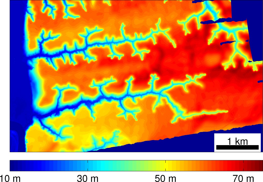
A kilometer-scale network of seepage valleys from the Florida Panhandle. These valleys are incised tens of meters into unconsolidated sand. Groundwater flows from the sand bed, through the channels, and through the bluff to the west of the network. Color indicates elevation above sea-level.
Réseau à l’échelle kilométrique des vallées drainant le « manche de poêle » de Floride (Florida Panhandle). Ces vallées ont incisé le sable non consolidé sur une dizaine de mètres. L’eau souterraine sourd des lits sableux, et s’écoule au travers des chenaux et de l’abrupt à l’ouest du réseau. La couleur indique l’altitude au-dessus du niveau de la mer.
This kilometer-scale network is incised into a 65-m deep bed of sand overlying an impermeable layer of muddy marine carbonates and sands (Schumm et al., 1995). The sand layer corresponds to the ancient delta of the Appalachicola river, which was deposited from Late Pliocene to Pleistocene (Rupert, 1991; Schmidt, 1985). The incision of ravines into the sand plateau probably started about 1 My ago (Abrams et al., 2009). This origin explains the remarkable homogeneity of the lithology, only perturbed by localized clay lenses. The vertical localization of the streams seems not to depend on stratigraphy (Schumm et al., 1995). Groundwater flows through the sand above the impermeable substratum, into the network of streams, and drains into a nearby river (Abrams et al., 2009; Schumm et al., 1995).
The dynamics shaping groundwater-fed networks are simpler than the more common type of drainage networks that are fed by overland flow. In particular, the flow of the groundwater into streams is determined by the shape of the water table, which is a solution to a Poisson equation (Bear, 1979). Because the growth of streams fed by groundwater is an example of network growth in a Poisson field, the analysis of landscapes shaped by this process benefits from a substantial literature on interface growth in a harmonic fields (Carleson and Makarov, 2002; Hastings and Levitov, 1998; Saffman and Taylor, 1958). Past work (Petroff et al., 2011) has shown that the flow of groundwater into the Florida network is accurately described by the Poisson equation.
Here we use the specific example of the Florida seepage network to explore the general connection between the geometry and growth of drainage networks. This exploration takes the form of four thematically-related, but independent, exercises in which the dynamic simplicity of seepage erosion is exploited to develop a quantitative understanding of field observations. The focus of this collection is the realization that groundwater flow and landscape erosion are coupled to one another by the stream network, and the empirical validation that, close to equilibrium, this coupling takes a simple form. Related oddities and novelties are also briefly discussed.
2 Estimating groundwater flow from network geometry
We first investigate the relationship between a heuristic geometrical model for groundwater flow and the Dupuit approximation (Bear, 1979), which is based on well-defined physical assumptions. We begin by considering a spring, the head of a stream where groundwater first reemerges to the surface. In particular, we compare two models that relate the position of a spring in the network to the flow of water into it. In the field site, we consider here, the ground surface is permeable enough to instantaneously absorb most of the rainfall. As a consequence, the water is transported to the stream almost exclusively as groundwater (Abrams et al., 2009; Schumm et al., 1995).
Our first model is the continuum model alluded to in the introduction. According to the Dupuit approximation of Darcy's Law (Bear, 1979), the water flux q is related to the height h of the water table above the impermeable layer as
| (1) |
| (2) |
Because the change in elevation along the Florida network is small (the median slope S ∼ 10−2), we approximate the height of the streams above the impermeable layer as constant. Because this equation is linear in the variable ϕ = Kh2/2P, this boundary-value problem around the streams of the Florida network can be solved using the finite element method (Hecht et al., 2005; Petroff et al., 2011).
The second model of subsurface flow is a heuristic geometrical model (Abrams et al., 2009). According to this approximation, all groundwater flows towards the nearest point on the stream network. Thus, to find the flux of water into a section of the network, one first identifies the area a around the streams that is nearer to the selected section than to any other point on the streams. This drainage area is not related to the topographic drainage area, which is commonly used to model surface runoff. From conservation of mass, the discharge of groundwater into this section is Qg = Pa.
Using these two models, we proceed to compare the estimated groundwater flux into 82 springs from the Florida network. To do so, it is useful to define the Poisson flux . Physically, qp is the area draining into a section of stream per unit length. By analogy, the geometric flux into a section of network of length δs and drainage area a is qg = a/δs. Because the area-driven model allows a finite area to drain into a point, this definition requires a finite value of δs; we take δs = 11 m. As shown in Fig. 2, there is a power law relationship (R2 = 0.94, p < 10−35) between these quantities, . The scaling exponent α = 0.69 ± 0.06. The proportionality constant, B = 4.0 ± 1.6 m1−α, likely depends on the choice of δs.
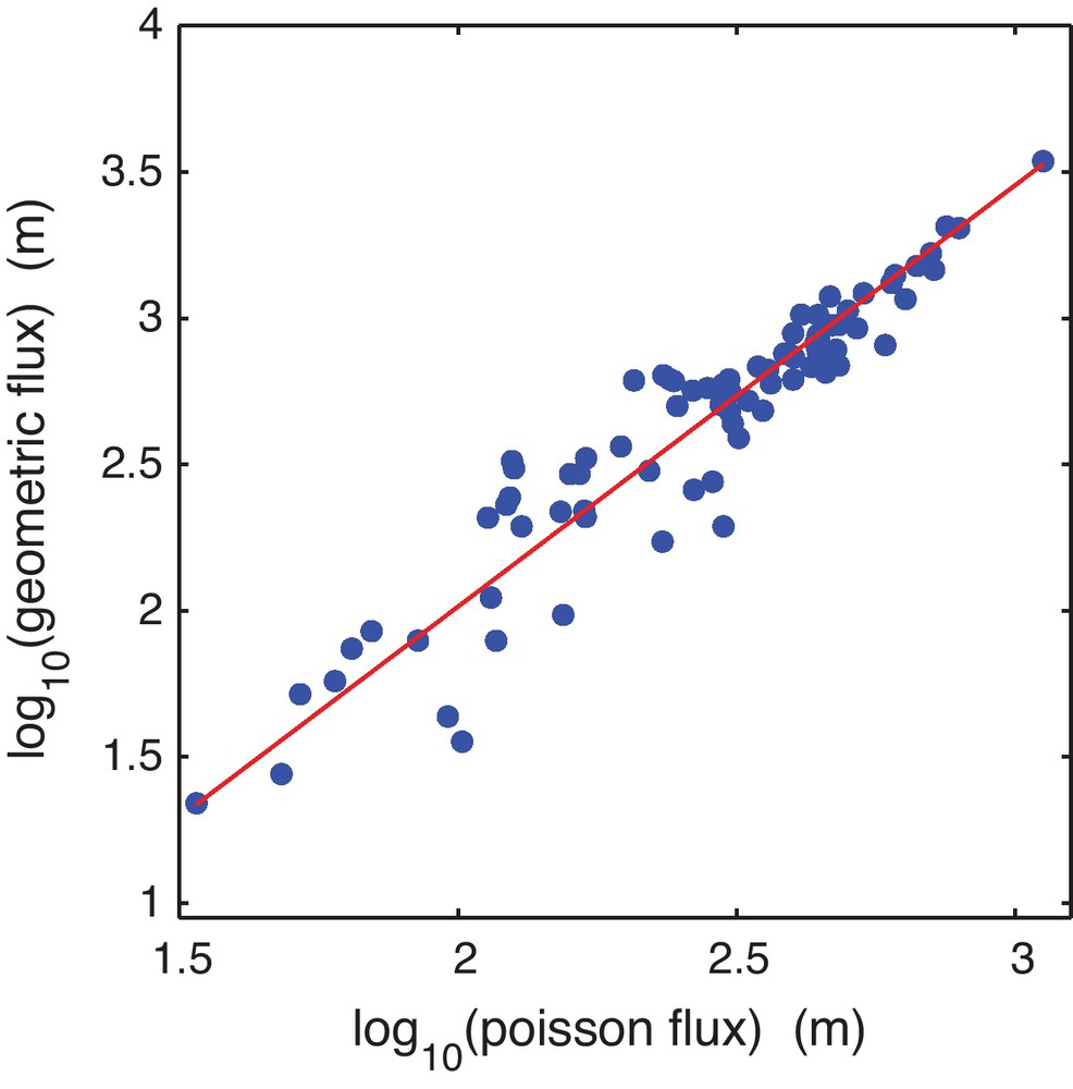
Comparison of the flow into 82 springs from the Florida network as estimated from Darcy's law (“Poisson flux”) and a heuristic model (“geometric flux” Abrams et al., 2009). The line shows the best fitting power-law.
Comparaison de l’écoulement de 82 sources du réseau de Floride, estimé d’après la loi de Darcy (« flux de Poisson ») et estimé à partir d’un modèle heuristique (« flux géométrique » Abrams et al., 2009). La ligne montre le meilleur ajustement d’une loi de puissance entre ces deux flux.
Although there is no general quantitative relationship between these measures, there is a formal relationship. Let us imagine that each rain drop falls randomly, with a uniform distribution over the domain, and then undergoes a random walk until it reaches a boundary. The probability distribution of the random walkers’ positions satisfies the Poisson equation, which can be interpreted as a diffusion equation with a uniform source term (Doyle and Snell, 1984). As a consequence of its random walk through the domain, this imaginary rain drop has a continuous and non-vanishing probability distribution p of exit locations along the boundary, with a maximum at the closest point on the boundary. The mean flux of walkers through the section of channels gives the Poisson flux. To find the geometric drainage area, one sends each random walker to the mode of p. Thus, the precise relationship between qg and qp depends on the geometry of the system and, consequently, the scaling exponent α relating these quantities is likely not universal.
We conclude that the area-driven model can be safely used as a conceptual tool with which to gain intuition. Nevertheless, the Poisson equation should be used whenever a quantitative prediction of the seepage intensity or the relative fluxes into different parts of the network is required.
3 The three dimensional structure of the network
Having discussed the flow of water into a stream, we now consider the response of sediment within the stream to the flowing water. Flowing water erodes the bottom of the sandy stream when the shear force exerted on a sand grain is sufficient to overcome friction. Thus, there is a threshold that the shear must exceed for any sediment to be transported. This threshold is often expressed as a function of the Shields parameter (which compares the grain weight to the flow-induced shear) in bedload transport laws (Sheilds, 1936; Vanoni and Keck, 1964). Many streams, and the Florida network in particular, are thought to adjust to a state in which every grain is on the threshold of motion (Devauchelle et al., 2011; Henderson, 1961; Lane, 1955). If we further approximate the stream with a straight and shallow channel formed in uniform sediment, the above constraint on the shear can be re-expressed as a relationship between the slope of the stream bed S and the discharge Q (units of volume/time) of water in the stream as
| (3) |
Because both the discharge of a stream and the slope affect the flow of groundwater into it, Eq. (3) imposes a boundary condition for the flow of groundwater into the streams, from which one can derive the profile of an isolated stream (Devauchelle et al., 2011). Here we show that this boundary condition is satisfied throughout the network.
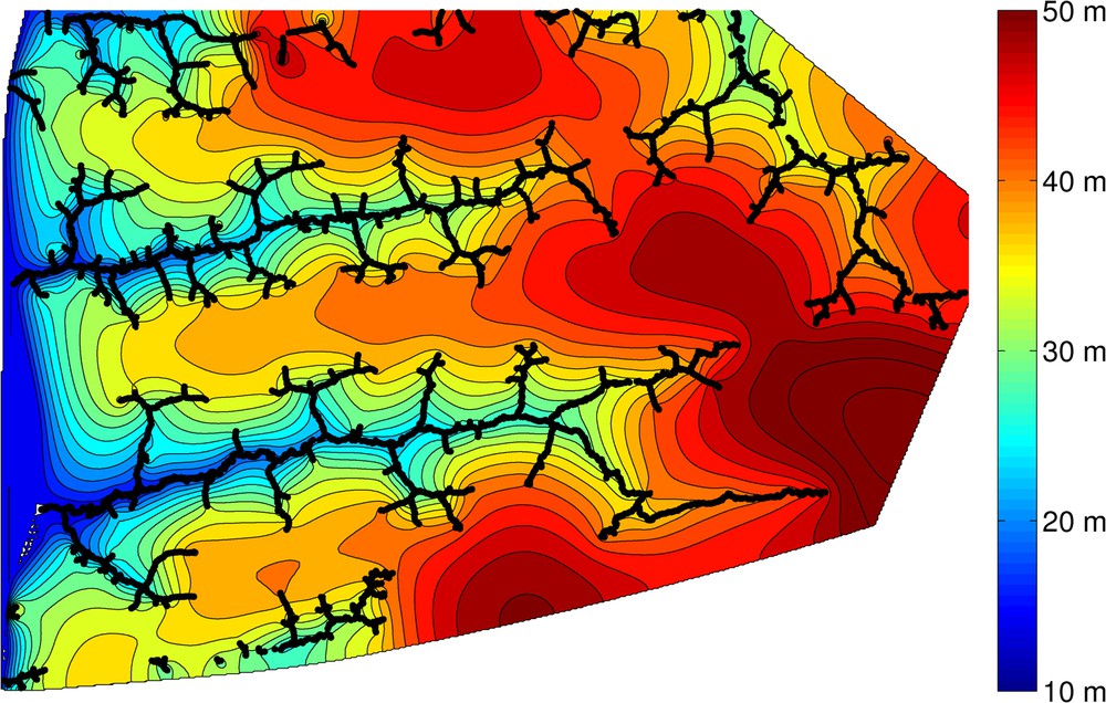
To test the applicability of Eq. (3), we compare the measured slope of streams to the stream discharge. Estimates of both the slope and the discharge require a three-dimensional description structure of the drainage network, which is extracted from the high-resolution topographic map of the network shown in Fig. 1. A depiction of part of the network is shown in Fig. 3. Given the height Hs of each point of the network, the slope is measured from the change in height along the stream. To estimate Q, we first solve Eq. (2) subject to the boundary condition on the streams
| (4) |

The three-dimensional shape of a stream network measured from a topographic map. Color indicates elevation above sea-level. Streams curve upward sharply near springs. Further downstream, as flow accumulates the streams become flatter. This inverse relationship between slope and discharge is in quantitative agreement with Eq. (3).
Forme tri-dimensionnelle d’un réseau fluviatile, mesurée à partir d’une carte topographique. La couleur indique l’altitude au-dessus du niveau de la mer. Les rivières s’incurvent très nettement à l’amont près des sources. Plus à l’aval, quand les écoulements se cumulent, les rivières deviennent plus plates. Cette relation inverse entre pente et débit s’accorde de manière quantitative avec l’Éq. (3).
Because Eq. (2) is a non-linear function of h, its solution depends on the height of the streams above the impermeable mudstone layer. The elevation of the impermeable layer above sea-level is h0 = 0. Fig. 4 shows the height of the water table around the network taking P = 5 × 10⁻⁸ m/s, K = 1.6 × 10⁻⁵ m/s. The value of the precipitation rate P corresponds to the yearly average rainfall in the concerned area. The value of the conductivity K was adjusted independently to match the distribution of discharges measured in the field (Petroff et al., 2011). Given this solution, Q is estimated throughout the network as
| (5) |
The shape of the water table around the Florida network as calculated from Eq. (2). Black lines represent the position of streams. The water table intersects the streams at the measured height of the stream. A zero-flux boundary condition is imposed along on the polygonal boundary encompassing the channels.
Forme de la surface de la nappe autour du réseau de Floride, calculée à partir de l’Éq. (2). Les lignes noires représentent la position des rivières. L’intersection de la surface libre de la nappe et des rivières s’observe à la cote mesurée de l’eau dans les rivières. Une condition aux limites de flux nul est imposée le long de la flimite polygonale extérieure du domaine englobant les chenaux.
Fig. 5 shows the comparison between the measured slope-discharge relation (blue points) and the quadratic relation predicted by Eq. (3). The value of Q0 is fit to the data and corresponds to a grain size of ds = 1.7 mm, consistent with observation. The slight disagreement between theory and observation at high and low values of discharge is likely the result of errors in the extraction of the network from the elevation map. The measurement of the discharge close to a spring is sensitive to the position and elevation of the spring in the network. The measured elevations of a substantial fraction of the springs are above the solution of the water table elevation, leading to a negative value of Q very close to the spring. The measurement of very small values of the slope is also affected by error in the original topographic map. Finally, the dependence of the friction coefficient on flow depth or the downstream fining of sediments can explain the slight overestimation of the exponent by the simplest version of the threshold theory.
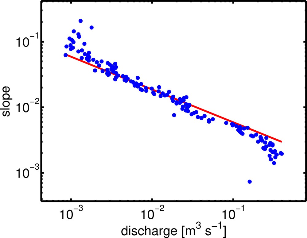
Comparison of the stream discharge to the slope. Discharge is estimated from the solution of Eq. (2) shown in Fig. 4. Slope is measured form the topographic map shown in Fig. 1. The line shows Eq. (3) assuming a grain size of 1.7 mm. Each point represents the average of 50 points in the network with similar discharges.
Comparaison du débit de rivière à la pente. Le débit est estimé à partir de la résolution de l’Éq. (2) représentée à la Fig. 4. La pente est mesurée à partir de la carte topographique de la Fig. 1. La ligne donne le débit calculé par l’Éq. (3) pour une taille de grain de 1,7 mm. Chaque point représente la moyenne de 50 points du réseau ayant des débits similaires.
The approximate agreement between theory and observation leads us to conclude that the streams throughout the network are poised at the threshold of sediment motion. The solution of Eq. (2) subject to boundary condition (3) determines the height of the streams throughout the network (Devauchelle et al., 2011).
4 Response of the surrounding topography
In the Florida network, streams are incised into a bed of unconsolidated sand. Since there is no surface runoff except for the streams themselves, the topography around them evolves as a function of slope only. The dependence of the sediment flux on slope is likely to be non-linear where the slope is close to critical. Far from the channels, however, we can represent the relaxation of the landscape by linear diffusion (Culling, 1960). We have not evaluated this hypothesis, but this assumption allows us to illustrate how the effect of sunlight on diffusion can be quantified. According to this hypothesis, the sediment flux j is related to the height of the topography H as
| (6) |
| (7) |
In general, D is determined by processes including rainfall, animal activity and vegetation. In this section, we consider variations in the diffusion coefficient (Bass, 1929; Burnett et al., 2008; Emery, 1947; Istanbulluoglu et al., 2008).
As shown in Fig. 6, the valleys cut by the drainage network are asymmetric; the southern valley wall is steeper than the northern wall. This asymmetry can be interpreted in two ways. Either there is a substantial north-south variation in the rate the landscape is diffusing or the the erosion rate is symmetric but the value of D is different. Because this network is in the Northern Hemisphere, the average position of the sun is to the south of the channels. Consequently, the southern walls of the valley are more shaded than the northern walls. Past studies have shown that there is a difference in vegetation between the northern and southern sides of the valley (Kwit et al., 1998).
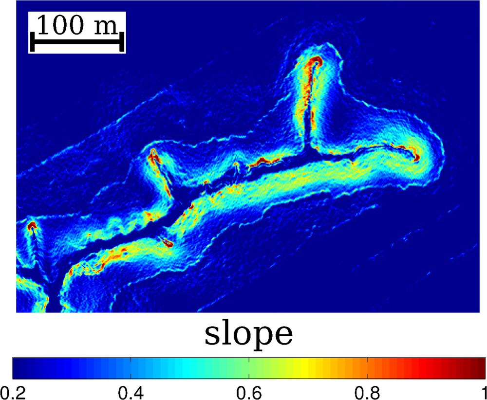
Map of slope in a section of the network. Slopes are systematically steeper on the southern side of valleys. The entire network was used in the analysis of the diffusion coefficient.
Carte de pente dans une section du réseau. Les pentes sont systématiquement plus fortes sur la partie méridionale des vallées. On a utilisé le réseau entier pour le calcul des coefficients de diffusion.
We characterize the influence of the sun with the projection of sun light onto the landscape. If is a unit vector pointing towards the sun and is the unit vector that is normal to the landscape at the point (x, y), the dimensionless light intensity is
| (8) |
It is straightforward to measure from the topographic map shown in Fig. 1. Given the latitude and longitude of the Florida network, the annual average solar zenith and azimuthal angles are 26.6° and 180° respectively (Reda and Andreas, 2004). Combining these values with Eq. (8) provides an estimate of I at each point in the field site.
We hypothesize that differences in average light intensity give rise to differences in D, resulting in asymmetric valley walls. Expanding D to first order in I gives
| (9) |
Here we estimate D1 from the shape of the topography assuming that there is no north-south asymmetry in the erosion rate. It is useful to express and I1 in terms of the orientation ω. Here, ω is defined as
| (10) |
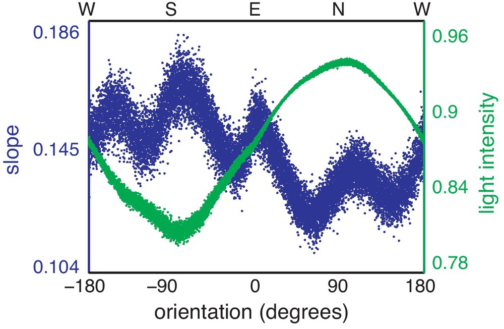
Variation of slope (blue) and light intensity (green) with orientation. The slope is systematically larger on the southern sides of valleys, where the light intensity is lower. The secondary structure in the dependence of slope on orientation reflects tendency of valleys to grow in the cardinal directions, as seen in Fig. 1. Each point represents the average of 1000 points from the topography.
Variation de la pente (en bleu) et de l’intensité de la lumière (en vert) en fonction de l’orientation. La pente est systématiquement plus forte sur la partie méridionale des vallées, là où l’intensité de la lumière est plus faible. La structure secondaire dans la dépendance de la pente à l’orientation reflète la tendance des vallées à se développer dans les directions cardinales, comme le montre la Fig. 1. Chaque point représente la moyenne de 1000 points de la topographie.
If there is no net asymmetry in the erosion rate, then
| (11) |
| (12) |
Combining the measured values of s and I from the Florida network with Eq. (12), yields D1 = 0.53 ±0.02. Thus, the fractional variation in the diffusion coefficient needed to account for the slope asymmetry is .
5 Growth of a stream
Having discussed the flow of groundwater into streams and the resulting adjustment of stream shape, and erosion of the landscape, we now turn our attention to the growth of a spring in response to the flow of groundwater. Because springs in the Florida network grow slowly, at a speed of ∼ 1 mm/year (Abrams et al., 2009; Schumm et al., 1995), this section relies on experimental observations.
Seepage channels are grown in a previously described experimental apparatus (Lobkovsky et al., 2007). In this experiment, a hydraulic head of 19.6 cm is used to push water through a bed of sand (grain diameter of 0.5 mm), having an initial slope of 7.8°. As water flows out of the sand bed, it entrains sand grains, thus forming a seepage channel. The channel is initialized with a small indentation in the otherwise flat bed of sand.
We characterize the growth of a channel by the shape of an elevation contour. A map of the experiment showing the shape of an elevation contour and its position in the experiment is shown in Fig. 8. Given this characterization, we ask how the growth of the contour outwards depends on the flux of water into it. To this end, we compare velocity of the contour with the solution of Eq. (2) around the channel.
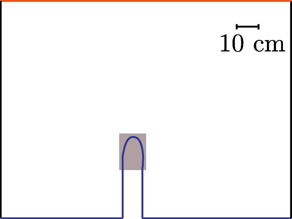
Schematic of channel growth in a table-top experiment after 30 min of growth. The growing channel head is shown in the gray square. Water flows from a reservoir (red line, where ψ = 1). Black lines show the position of impermeable walls (∂ψ/∂n = 0). Blue lines at the base show the position of a second reservoir (ψ = 0).
Schéma de naissance d’un chenal dans une expérience en laboratoire après 30 min de croissance. La tête du chenal en croissance est représentée par le carré gris. L’eau s’écoule d’un réservoir en amont (ligne rouge, où ψ = 1). Les lignes noires indiquent la position des murs imperméables (∂ψ/∂n = 0). Les lignes bleues montrent la position d’un second réservoir à l’aval (ψ = 0).
The normal velocity of the contour is measured by comparing the shape of the contour to its shape a moment later. Given an elevation, we determine the normal vector at each point along the associated contour. We then compare the shape of a contour to the shape of the same contour three minutes later to determine the amount that each point on the contour grew in the normal direction. Two elevation contours at three minute intervals are shown in Fig. 9.
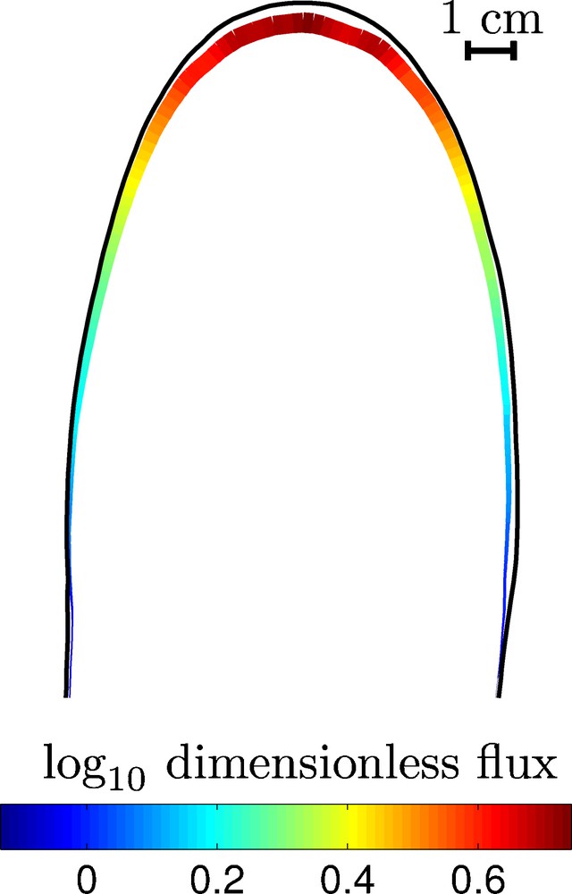
Channel growth in a table top experiment. A detail (gray square in Fig. 8) of the growing channel head elevation contour. Color represents the flux of water into the boundary. The solid black line shows the position of the channel three minutes later.
Croissance d’un chenal dans une expérience en laboratoire. Détail (carré gris sur la Fig. 8) de la ligne d’égale altitude de la tête du chenal en croissance. La couleur représente l’intensité du flux d’eau arrivant au chenal. La ligne noire continue montre la position du chenal trois minutes plus tard.
To determine the flux of water entering each part of the channel, we solve for the shape of the water table. In these experiments, there is no rainfall, thus Eq. (2) simplifies to the Laplace equation
| (13) |
As shown in Fig. 10, the velocity at which the channel grows outward is linearly related to the flux of water into it. This is unexpected, as typical transport relationships relate sediment transport to shear nonlinearly. Moreover, according to the least-squares fit of the data, the intercept of this relationship is negative, meaning that a finite flux of water is required for the channel wall to grow forward. This result is superficially similar to the finite shear required to transport sediment in a stream (Sheilds, 1936; Vanoni and Keck, 1964). Because the growth of the channel requires that sediment be transported through the channel, this relationship between flux and growth does not reflect a simple force balance on a sand grain. Rather, this relationship arises from the coupling between sediment transport within the channel and subsurface flow around the channel. It is therefore remarkable that this relationship takes a form in which the growth at a point depends only on the flux at that point. As the channel wall height remains roughly constant during the experiment, this result implies that the increase in the network volume is roughly proportional to the total delivery of water (neglecting the channel sides, where the water flux is small).
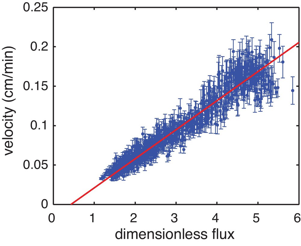
Comparison of the normal velocity of the channel to the flux of water into it. The dimensionless flux is found by solving Eq. (13) around the measured shape of a channel. The velocity is measured from changes in the shape and position of the channel.
Comparaison de la vitesse normale dans le chenal au flux d’eau qui lui parvient. Le flux adimensionnel est calculé par résolution de l’Éq. (13) autour de la forme mesurée d’un chenal. La vitesse est mesurée à partir des changements de forme et de position du chenal.
6 Discussion
This collection of remarks has been arranged so as to connect – the way a skipping stone connects the banks of a wide river – the flow of groundwater through the aquifer to the flow of sediment over the landscape. We began, in section 2, by relating a heuristic model of subsurface flow to Darcy's law. In section 3, we showed that the boundary condition for the flow of groundwater is determined by the condition that sand grains in the streams are at the threshold of motion; this boundary condition determines the height of streams (Devauchelle et al., 2011). In section 4, we proposed a method to measure the influence of sun exposure on landscape diffusion from topographic data. Finally, in section 5, we showed that the local erosion rate of experimental seepage channels is linearly related to the water flux, beyond a threshold value.
We now pause to consider the metaphoric “wide river”. The first three results represent three aspects of a single boundary value problem specified by the principal equations of these sections,
| (14) |
| (15) |
| (16) |
| (17) |
Given the current shape of the landscape, these equations describe the evolution. It is an open question if this set of equations describes the advance of the spring. In particular, we ask if the observed relationship between channel growth and groundwater flux in section 5 represents a fourth aspect of this boundary value problem.
The answer to this question deeply influences our conceptualization of how drainage networks grow. If these equations are complete, network growth represents a balance between the accumulation of water in the streams and the erosion of the surroundings. In this case, sediment transport is simply the mechanism that maintains this balance. If these equations are not complete, the way a network grows and the surrounding landscape changes depend on the details of how sediment moves through the network. Once this question is answered, the details of this model can be adapted to suit the details of a more complex world.
Acknowledgments
We would like to thank The Nature Conservancy for access to the Apalachicola Bluffs and Ravines Preserve, and K. Flournoy, B. Kreiter, S. Herrington and D. Printiss for guidance on the Preserve. Thanks to D.M. Abrams and H. Seybold for fruitful discussions. We thank B. Smith for her experimental work. Finally, we thank the referees C. Paola, P. Davy, S. Douady and Y. Couder for their careful reviews, which helped us improve and clarify the manuscript.
This work was supported by Department of Energy grant FG02-99ER15004. O. D. was additionally supported by the French Academy of Sciences. A.K. was additionally supported by Department of Energy grant FG02-02ER15367.