

1 Introduction
The development of computer science has greatly enhanced the use of numerical methods to provide solutions of the flow equation of natural groundwater systems. Recent trends on groundwater models dealing with heterogeneity (Marsily et al., 2005) underline this fact. Unfortunately, increasing grid resolution increases the size of the corresponding matrix equations.
To face this problem, earlier flow solvers used the method of successive over-relaxation to accelerate the convergence of Southwell's original relaxation matrix (1946). Nevertheless, a quick analysis shows that a meaningful representation of the variability of the logarithmic transmissivity implies a computational requirement which involves a number of finite difference blocks N on the order 104 for a two-dimensional flow and of 106 for a three-dimensional one (Ababou et al., 1985).
That is to say that, respectively 106 and 109 iterations are needed to reach this numerical accuracy with SOR whose convergence grows as N3/2, whereas the convergence of multigrid methods grows as N log N and involves 4 × 10⁴ and 6 × 10⁶ iterations.
Consequently, standard numerical methods are unpractical in terms of time and storage to tract such matrix sizes, which is why most groundwater modelling software is now using preconditioned conjugate gradient methods (Hill, 1990) and multigrid methods (Mehl and Hill, 2001; Stüben and Klees, 2005) which can give a new use to SOR as a preconditioner.
However, it is a matter to regret that these new solvers are less users-friendly despite the increasing conviviality of the current software packages and the potentialities of the new graphical user interfaces. Currently, the context-sensitive help given in these packages to users unfamiliar with groundwater modelling refers still to textbooks such as Chiang et al. (1998).
An easy-to-use governing criterion for the selection of a preconditioner to the flow solvers remains a sensitive question for the users.
This article attempts at giving a preliminary response to some of these perceived weaknesses. A qualitative geological concept is linked to a mathematical one in order to provide an understanding of the numerical solver in a manner that will enable users of groundwater models to make these choices based on their original background, i.e. geology.
We will use SOR to support the illustration of this task for four reasons:
- • its simplicity allows us to give a straightforward idea on the relationship between statistical hydrogeological parameters and convergence issues;
- • SOR is still an efficient iterative stand-alone solver for small-size problems, as was very well shown by Ehrlich (1981);
- • SOR is an effective preconditioner for Preconditioned Gradient (PCG) methods handling symmetric successive over-relaxation (SSOR);
- • contrary to existing belief, SOR may be a suitable smoother (Popa, 2008) in the strategy of multigrid dealing with moderate anisotropy (Yavneh, 1996) or for solving 2-D Poisson equations (Zhang, 1996).
Investigating the efficiency of SOR as a stand-alone solver, as a preconditioner and as a smoother for heterogeneous fields is the subject of this article. The smoothing property is only formally examined herein. It will be experimented in further work. In the following, Monte Carlo simulations are performed to compute the spectral radii of flow matrices arising in groundwater flow modelling through multiple replications of a non-homogeneous aquifer. These are considered as different equiprobable realizations of a random function. Inspection of the optimal relaxation factor of the SOR method is pursued following an analytical determination in the homogeneous case and through the Young formula in the heterogeneous case. Then, variations of the optimum relaxation factor are expressed as a function of the standard deviation of the logarithm of the transmissivity field Y and parameterized on the correlation lengths of this field.
2 On the flow model
In steady state conditions, the groundwater flow is described by Poisson's equation (Bear, 1972):
| (1) |
In Eq. (1) h is the dependant variable, the hydraulic head, and T is a distributed parameter called transmissivity, whereas q is a source term. The equivalent finite difference form of Eq. (1), derived with the centred difference scheme, can be compacted, and expressed in matrix notation (Golub and Van Loan, 1996) as:
| (2) |
A quick inspection of B shows that it is a real irreducibly diagonally dominant symmetric matrix with negative diagonal entries and non-negative off-diagonal entries.
3 Preliminary numerical considerations
3.1 On the numerical solver
When a numerical solver of Eq. (1) is selected, it needs to be efficient for solving the set of linear algebraic Eq. (2). Although SOR performs well for small-size problems, it cannot efficiently solve large ones. However, it is useful to evaluate its efficiency either as a convergence accelerator in PCG or as an error smoother in multigrid algorithms.
3.2 Optimized relaxation
SOR may be defined from the regular splitting of the flow matrix B:
| (3) |
Then the iterated heads are:
| (4) |
with the parameter ω as relaxation factor. They are generated with the over-relaxation matrix:
| (5) |
| (6) |
| (7) |
| (8) |
Therefore, SOR would be a fair way to increase the convergence rate of the iteration matrix £ω if the relaxation factor ω was chosen according to Kahan's theorem, i.e. in the interval]0, 2[and near its optimal value ωopt. The convergence rate may even be faster than the convergence rate of the symmetric successive over-relaxation method (SSOR) which combines two successive SOR sweeps together, one performed with the matrix £ω (forward sweep), the second one with the same matrix £ω but with the roles of E and Et reversed (backward sweep).
Practically, both convergence rates of SOR and SSOR may deviate from the optimum when ω is greater than ωopt. Then, either oscillations occur, as the head change repeatedly reverses to compensate for the overshoot, or convergence slows down monotically or worse becomes degenerate in that the closure criterion is not satisfied everywhere. This should be kept in mind when regarding the choice of ω, otherwise there would be little understanding of why one value of ω performs better than another.
For simple problems, this value of ωopt could be computed from Young's formula:
| (9) |
| (10) |
Let ρ(J) = 1–10–4 then by (9) ωopt = 1.972. An estimate ω = 1.9 would reduce by seven the rate of convergence of the iteration matrix £ω.
3.3 Preconditioning for conjugate gradient
When solving (2), conjugate gradient methods are known to yield the exact result after n iterations. In the hypothetical context of infinite floating point precision, this number is at most equal to the number of distinct eigenvalues. The convergence is even faster when these eigenvalues are clustered together. A well-known result on convergence issue states that:
| (11) |
To reduce the norm of the error by a factor ɛ, that is:
| (12) |
the maximum number of iterations required is:
| (13) |
That it is to say, Nω is bounded by a constant times the square root of the condition number.
The complexity of the CG method is evaluated through the number of matrix-vector multiplications, which is of order whereas that for condition number γ(B) is O(n). Thus, the complexity for CG used to solve a two-dimensional problem (2) is of order .
According to this, CG methods should almost always be used with a preconditioner for large scale-applications. The resulting matrix noted M–1B should be much better conditioned than B or its eigenvalues should be better clustered, i.e. with less distinct ones. Finding such preconditioners is an ongoing research (Saad, 2000).
Following is an illustration of the improvement:
- • that SOR brings to the Gauss-Seidel (GS) iterative method when an optimal acceleration factor is used and;
- • that a diagonal preconditioner effectively brings to reduce the rate of convergence of the flow matrix involved in the numerical experiments (Table 1).
Influence du pas d’espace sur les caractéristiques spectrales de la matrice B, de la matrice de Jacobi (J) et de la matrice préconditionnée (D−1B).
| M | 6 | 9 | 14 | 24 | 31 | 36 |
| ρ(B) | 7.604 | 7.804 | 7.913 | 7.968 | 7981 | 7.990 |
| 7.604 | ||||||
| γ(B) | 19.80 | 39.86 | 90.52 | 252.6 | 414.3 | 1053 |
| 19.20 | ||||||
| 0.63 | 0.73 | 0.81 | 0.88 | 0.91 | 0.94 | |
| 0.63 | ||||||
| ρ(J) | 0.901 | 0.951 | 0.978 | 0.992 | 0.995 | 0.998 |
| 0.901 | ||||||
| 1.395 | 1.528 | 1.655 | 1.776 | 1.818 | 1.881 | |
| 1.395 | ||||||
| ρ(D−1B) | 1.901 | 1.951 | 1.978 | 1.992 | 1.995 | 1.997 |
| 1.901 | ||||||
| γ(D−1B) | 19.80 | 39.82 | 89.92 | 248.99 | 399.0 | 991.0 |
| 19.20 | ||||||
| 0.63 | 0.73 | 0.81 | 0.88 | 0.90 | 0.94 | |
| 0.63 |
3.4 Smoothing in multigrids
The fundamental idea behind multigrid algorithms (Stûben, 1999) is to process a sequence of relaxations — transfers to successively coarser grids and then to get back to finer grids in a recursive way corresponding to what is known as a V-cycle. The smoother plays a key role in this strategy. Usually it is chosen among the classical iterative methods provided that it satisfies a so-called smoothing property. The SOR method satisfies this smoothing property (Popa, 2008) for a constant α ≥ 0 such that:
| (14) |
The constant α ≥ 0 is given by:
| (15) |
The aim of relaxation is to smooth errors rather than to reduce them. Many relaxation schemes have this smoothing property, i.e. filtering the oscillatory Fourier modes and damping the smooth ones. Coarsening lets these modes appear more oscillatory. Thus, on coarser grids, relaxation will be more effective on these modes.
Although using a relaxation parameter may improve the smoothing property, it has been carefully avoided because the V-cycle does not appear to be sensitive to acceleration for the Laplace operator. In fact, an efficient use of a relaxation parameter in a V-cycle should be performed under-relaxation during the first cycle and over-relaxation during the second one. This cross-use of under-relaxation and over-relaxation avoids smoothing to deteriorate and may induce a slight improvement in the smoothing properties (Zhang, 1996). Thus, a SOR smoother as presented in Eq. (8) may improve the Gauss-Seidel smother (6) although it is quite sensitive to the choice of ω. The storage requirement of a V-cycle is on the order of that of the fine grid. It increases only linearly with the problem size. The computational cost for obtaining a solution whose error is on the order of the discretization error is O(n2Log n).
This is clearly much better than that required by standard iterative methods.
Further, statistical results are provided through Monte Carlo simulations.
4 Monte Carlo simulations and the transmissivity geostatistical model
The geostatistical terminology characterizes the transmissivity as a regionalized variable which may be described by a small number of statistical parameters (Gehlar, 1993). Usually, the mean, the variance and the correlation length are sufficient to represent such variables. The aforementioned characterization is enhanced by using the consensual lognormal probability density function (pdf) Y = Log T (Gehlar, 1993).
The geostatistical model of heterogeneities is thus summarized by the pdf of Y and its autocovariance function, both used to infer how the values of Y correlate in space and to represent the spatial continuity in the distribution of Y. The exponential autocovariance model is adopted here, although several others well-established models allow a comparable level of flexibility (Gehlar, 1993):
| (16) |
According to (16), the correlation length scale lY is the distance at which the autocorrelation function takes a value of e−1.
Defined in this way, heterogeneity and correlation lengths are such that:
- • a low variability occurs within one correlation length;
- • an estimated value of Y within one correlation length fluctuates less and varies less than over several correlation lengths.
Long correlation length (i.e. small αY) will represent low heterogeneity for Y whereas shorter correlation length (i.e. larger αY) will express higher heterogeneity for Y. Such a representation of Y has greatly stimulated the development of techniques to generate synthetic equiprobable Y-fields with prescribed geostatistical properties. An up-to-date improvement of such random field generators is described by Fenton (1990).
Monte Carlo simulations are used successively with Eq. (3) and such synthetic matrices B in view to examine the variations of the over-relaxation coefficient ω as a function of the heterogeneities of the log T field.
5 Numerical experiments
The numerical experiments were performed on a non-dimensional form of Eq. (1):
| (17a) |
| (17b) |
The associated boundary conditions are:
| (17c) |
The homogeneous case is the starting point of the numerical experiments performed with Eqs. (17). Then, the impact of the heterogeneity of the Y-fields on the optimum relaxation factor is explored by varying both the values of the standard deviation σY and the correlation coefficient αY. The chosen values are typical of slowly variable fields. In this case, σY are taking values in the interval [0.0, 2.0] incremented by 0.2, whereas 0 ≤ αY ≤ 1 for correlated fields. Uncorrelated fields are generated with α → ∞ corresponding to a correlation length scale lY = 0.
5.1 Homogeneous fields
The only case where the evaluation of the optimum relaxation factor can be made directly is the one dealing with a rectangular grid domain (p, q). It allows one to verify the algorithms used for the numerical computations of ρ (B) and ρ (J). The spectral radius of B is given by an analytical formula which takes the form:
| (18) |
| (19a) |
| (19b) |
The analytical expression of the optimal acceleration parameter derived with this value of
ρ (J) reduces to:
So far, the numerical results for N = 6 agree with those obtained with the expressions (18), (19b) and (20) reported in column 2 of Table 1. For the other space increments, the values of the spectral radii ρ(B), ρ(J) and the associated ωopt are just computed to infer their behavior with respect to N.
The optimum relaxation factor appears to increase when the mesh size decreases, in agreement with the expressions (10) and (20). Indeed, it lies in the interval]0,2[.
The above result may be illustrated once again by examining the performance of SOR. Let NIT be the number of iterations measured to reach the precision ɛ = 10–8 satisfying the closure criterion and Vω the asymptotic rate of convergence, then since:
The product V × NIT should be near –Log ɛ = 18.42 whenever ω ≠ ωopt. The results are presented in Table 2. Only the row corresponding to ω = ωopt differs, since for ωopt = 1.39 the value of Vω × NIT (24.15) is greater than –Log ɛ.
Performances numériques de SOR pour différentes valeurs du coefficient de surrelaxation.
| ω | ρω | V ω | 1/Vω | NIT | Vω × NIT | % 1/Vω | % NIT |
| 1.00 | 0.8118 | 0.2085 | 4.7960 | 76 | 15.85 | 4.45 | 4.00 |
| 1.30 | 0.6288 | 0.4639 | 2.1556 | 38 | 17.63 | 2.02 | 2.00 |
| 1.35 | 0.5612 | 0.5776 | 1.7313 | 32 | 18.48 | 1.61 | 1.68 |
| 1.39 | 0.3950 | 0.9289 | 1.0766 | 26 | 24.15 | 1. | 1.37 |
5.2 Heterogeneous fields
In all the other cases but the last one, the spectral radius ρ (B) is unknown. Then, the optimum relaxation factor ωopt should be determined from Young's relationship via the determination of ρ (J).
In the following application, the determination of the spectral radius is performed with Matlab. To perform these computations, matrix B is given with entries generated by the LLt decomposition scheme. Fig. 1 depicts the results for some of the Monte Carlo simulations of these autocorrelated fields. They summarize the influences of both the standard deviation, σY and the correlation length lY on ωopt.

Effect of the correlation length on the log T field (a) N (0, 0.2, 01) (b) N (0, 0.2, 09).
Effet de la longueur de corrélation sur le champ de log T (a) N (0, 0.2, 01) (b) N (0, 0.2, 09).
6 Results
Fig. 2 describes the variation of ωopt with the standard deviation and the correlation length, compared to the one computed for the homogeneous field N(0; 0.0, 2.0). Only a few values of ωopt, typical of some realizations of the random function Y, are extracted from the population N(0; σY, lY). The CPU time needed to solve Eqs. (17) with the optimized SOR method is increasing with the standard deviation σY.

Influence of the over-relaxation on the CPU time.
Influence de la surrelaxation sur le temps CPU.
Overestimation of ωopt of a given amount increases the CPU time less than an underestimation of ω by a same amount. This behaviour is re-enforced when σY increases. This variation of ωopt anticipates its evolution shown on Fig. 3 where it can be seen that ωopt increases when heterogeneity σY increases. For the simulated heterogeneous fields, the optimal over-relaxation factor lies between 1.397 and 1.707.
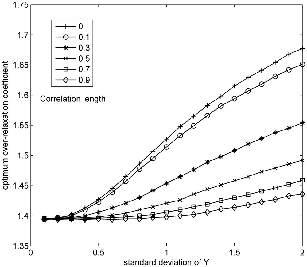
Influence of the standard deviation on the optimum coefficient of over-relaxation.
Influence de la déviation standard sur le coefficient de surrelaxation.
On the contrary, the correlation length of Y acts in the opposite direction than the standard deviation σY. An increase of heterogeneity due to a decrease of the correlation length increases the values of ωopt. For weakly heterogeneous and strongly correlated fields (0.5 ≤ lY ≤ 0.9), ωopt varies much less with the correlation length. For uncorrelated fields, ωopt varies much more with σY than for correlated fields.
Fig. 4 displays the error-bars associated with the experimental results of Fig. 3. It shows an increase of the spread on the estimates ωopt around the mean value when the standard deviation σY increases. This spread increases as the correlation length decreases (Fig. 5). This larger spread is due to the larger dispersion of the spectral radius observed when σY increases. It would be smaller if a greater number of realizations had been used in the numerical experiments.
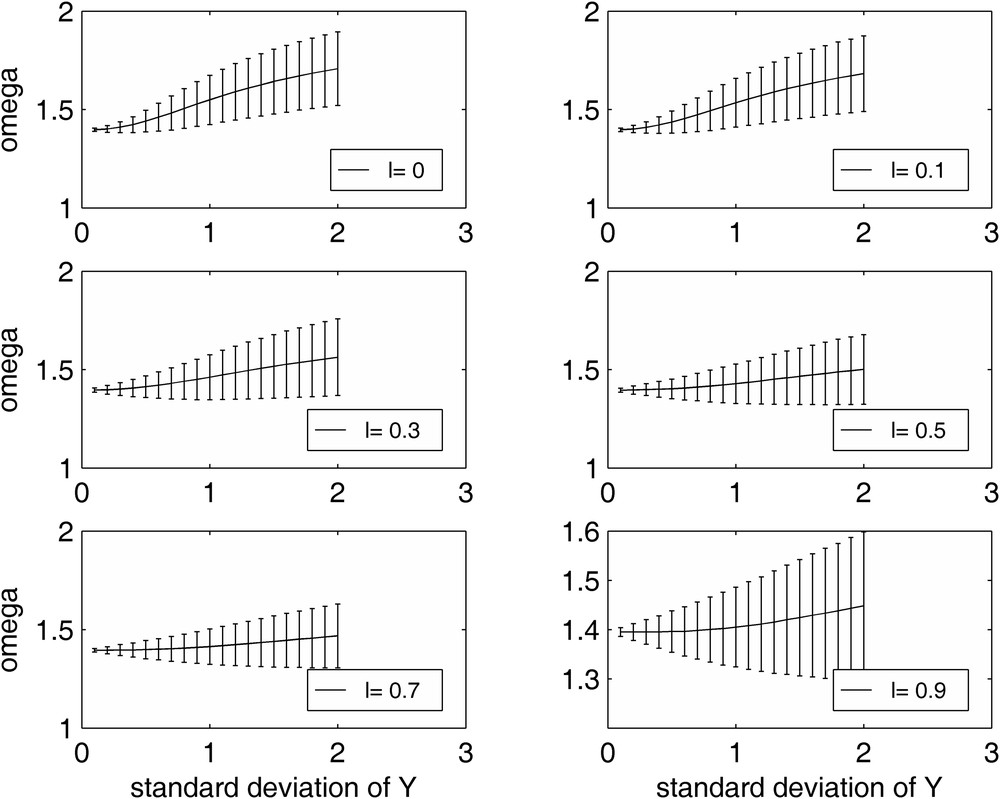
Error bar on the optimum over-relaxation factor for different correlation lengths.
Intervalle de variation du coefficient de surrelaxation optimal pour différentes valeurs de la longueur de corrélation.
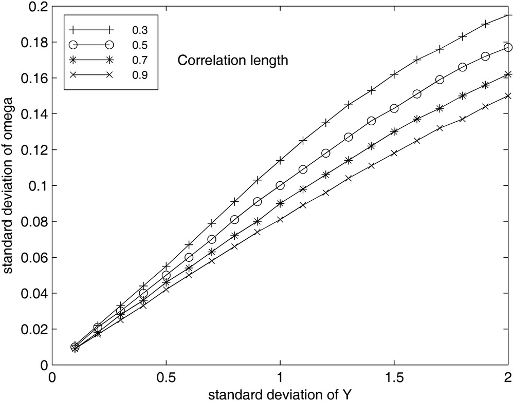
Influence of the standard deviation of Y on the standard deviation of ωopt for different correlation lengths.
Influence de la déviation standard de Y sur la déviation standard de ωopt pour différentes longueurs de corrélation.
6.1 Influence of the sample size
The recurrent critical question addressed by Monte Carlo sampling deals with the number of realizations required to obtain a reliable estimate of the optimal over-relaxation factor. This number is likely to depend on the problem and on the heterogeneities incorporated into the model. A general rule often used is to reach ergodicity by performing computations until some ensemble statistics do not significantly change. Then, a consensual rule-of-thumb is to stop the simulations when the standard error of the mean, , is less than 1%. With NR = 200 runs, this rule implies σω ≤ 0.14.
A Latin Hypercube sampling would achieve the same degree of accuracy with much less trial runs than the conventional Monte Carlo sampling used here. Nevertheless, the dependence of the standard deviations of the optimal over-relaxation factor on the standard deviation of Y (Fig. 6) confirms the dependence of NR on the heterogeneity of the Y field. Fortunately, additional computations made with 300 and 400 realizations do not really change the results obtained with NR = 200. Table 3 reports the values of the optimum over-relaxation coefficient computed for some transmissivity fields. They confirm the good stability of the statistics made on ωopt since the ratio of the asymptotic convergence rates R=Vω/V200 is not very sensitive to the sample size and is stable around 1.25.
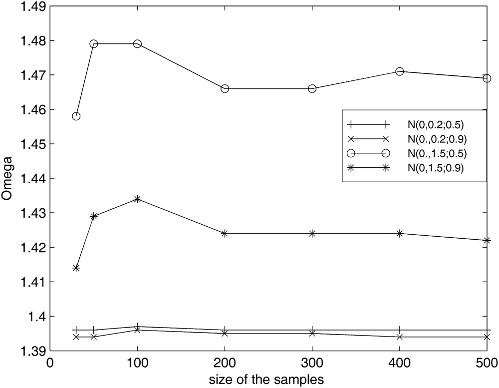
Influence of the number of realizations on the optimum over-relaxation factor.
Influence du nombre de réalisations sur le coefficient de surrelaxation optimal.
Influence du nombre de réalisations sur le coefficient de surrelaxation optimal moyen (σY = 0.1;0.3 lY = 0.5;0.7).
| Number of realizations | |||||||
| 30 | 50 | 100 | 200 | 300 | 400 | 500 | |
| ω25 | 1.396 | 1.396 | 1.397 | 1.396 | 1.396 | 1.396 | 1.396 |
| V ω | 0.926 | 0.926 | 0.924 | 0.926 | 0.926 | 0.926 | 0.926 |
| R | 1 | 1 | 0.998 | 1 | 1 | 1 | |
| ω 29 | 1.394 | 1.394 | 1.396 | 1.395 | 1.395 | 1.394 | 1.394 |
| V ω | 0.931 | 0.931 | 0.926 | 0.929 | 0.929 | 0.931 | 0.931 |
| R | 1.002 | 1.002 | 0.997 | 1. | 1.002 | 1.002 | |
| ω 155 | 1.458 | 1.479 | 1.479 | 1.466 | 1.466 | 1.471 | 1.469 |
| V ω | 0.781 | 0.736 | 0.736 | 0.764 | 0.764 | 0.753 | 0.757 |
| R | 1.022 | 0.963 | 0.963 | 1. | 0.986 | 0.991 | |
| ω 159 | 1.414 | 1.429 | 1.434 | 1.424 | 1.424 | 1.424 | 1.422 |
| V ω | 0.881 | 0.846 | 0.835 | 0.858 | 0.858 | 0.858 | 0.863 |
| R | 0.974 | 0.986 | 0.973 | 1. | 1. | 1.001 |
6.2 Influence of the mesh size
There is no significant difference with respect to the observations already made for the homogeneous field: a slowly increasing shape of the spectral radius ρ (J) with the grid resolution induces an increase of ωopt (Fig. 7). This increment seems linear for homogeneous fields while it deviates from a linear shape once heterogeneities are incorporated in the model (8). This deviation seems minor since a least-squared straight line might still be drawn if more data were provided.
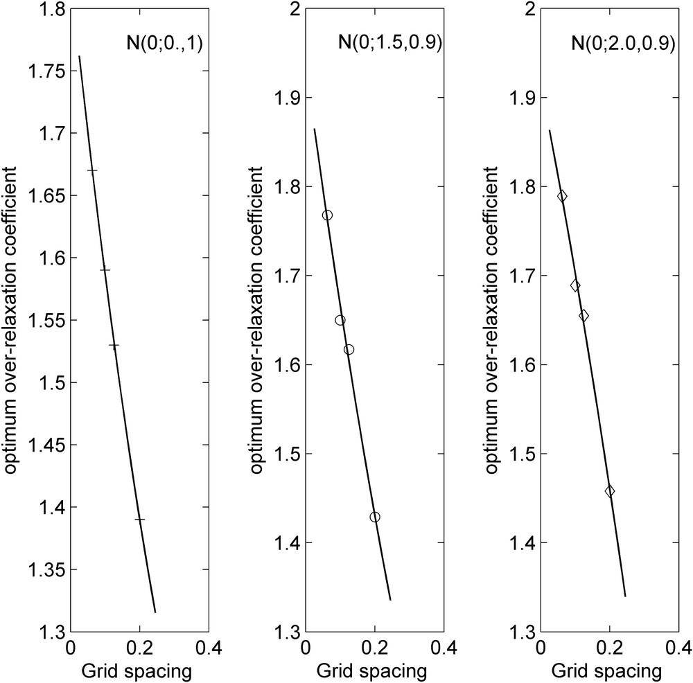
Effect of grid spacing on the optimum over-relaxation factor (homogeneous and heterogeneous Y-fields).
Effet du pas d’espace sur le coefficient de surrelaxation optimal (cas homogène et cas hétérogène).
6.3 Functional relationship
The optimal over-relaxation coefficient ωopt appears as being a function of the standard deviation σY, of the correlation length lY and of the mesh size a = Δx. For a given configuration of the mesh, this function may be approximated by a polynomial expression of the 5th degree in σY:
| (21) |
whose coefficients pi are a function of the correlation length. The discrete values of these functions are given in Table 4 for σY increasing from 0 to 0.9. The influence of the mesh size may even be incorporated in the expressions of pi as a mixed-polynomial in lY and Δx.
Coefficients de la relation fonctionnelle de ωopt.
| l y | p 1 | p 2 | p 3 | p 4 | p 5 |
| 0. | 0.04483 | −0.2418 | 0.4169 | −0.07128 | 1.4 |
| 0.1 | 0.03713 | −0.2054 | 0.3641 | −0.0625 | 1.4 |
| 0.3 | 0.008414 | −0.06146 | 0.144 | −0.02676 | 1.397 |
| 0.5 | −0.003455 | −0.0005301 | 0.04549 | −0.008926 | 1.396 |
| 0.7 | −0.00306 | 0.02592 | 0.02592 | −0.01034 | 1.396 |
| 0.9 | −0.004023 | 0.01313 | 0.005726 | −0.005724 | 1.396 |
6.4 SSOR as a preconditioner
The performance of the preconditioned conjugate gradient method depending heavily on the preconditioner and in turn on the condition number, a comparison was made for increasing heterogeneities. Two preconditioners are tested: Jacobi and Evans (SSOR).
Fig. 8 shows the variations of the condition numbers of the corresponding preconditioned matrices. The data are those of the uncorrelated field since the influence of the standard deviation σY, of the correlation length lY and of the mesh size a = Δx are already known.
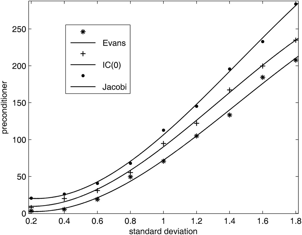
Comparative shape of Evans and Jacobi preconditioners.
Evolution comparée des préconditionnements d’Evans et de Jacobi.
The condition number of the SSOR preconditioner is smaller than for the Jacobi preconditioners. Fig. 8 shows the efficiency of SSOR as the standard deviation of Y increases. Hence, as could be expected, once an optimal value for ω is available, the SSOR preconditioner provides a faster rate of convergence than the Jacobi preconditioner. The number of iterations is thus reduced. As mentioned earlier, SSOR is given in a factored form, so since it is given a priori, there is no possibility of breakdown as in the phase of construction in the incomplete factorisation methods.
On Fig. 9, the flow model represented by Eq. (17) is solved successively with PCG, preconditioned with SSOR and with optimized SOR. The improvement that SSOR brings to the conjugate gradient method is much more important than optimizing the SOR used as a stand-alone solver.

Comparative rate of PCG (Evans) and SOR optimized.
Evolution comparée des vitesses de PCG (Evans) et SOR optimisée.
6.5 SOR as a smoother
Early applications of SOR as a smoother in a multigrid strategy did not discriminate between low and high-frequency modes although restriction and interpolation do not affect them in the same way. Thus, the gain in one half cycle of the V-cycle is lost in the second one. According to the value of the over-relaxation coefficient ω, the reduction factor μ accelerates either the reduction of the low-frequency errors or the reduction of the high-frequency ones.
Following Zhang (1996), under-relaxation with values of ω between [2/3,1] accelerates the reduction of the low-frequency errors, and over-relaxation with values of ω between [1,5/4] accelerates the reduction of the high-frequency errors. Our results show a link between ω and σY i.e. between μ and σY which makes us believe that SOR may be a suitable smoother in the smoothing strategy of multigrid applied to weak heterogeneity.
7 Application
Due to the importance of good estimates of ωopt on the performance of the numerical solver SOR, we attempted to tailor an available groundwater flow model to this individual need by modifying and adding menus to the user main menu. The programs that we added incorporate DATAPREP to read data used by PREVAR to pre-process VARIO which is a variogram analysis and modelling program of the US-EPA (Englund and Sparks, 1991). This package provides the parameters σY and lY of the field. Then Fig. 2 allows the evaluation of the correct optimum relaxation factor as a function of these values. In fact, we have to deal with σY and lY, which concern the gridded data. So, it would be better to use KRIGE after VARIO to produce the sample of input data, then to run PREVAR and VARIO once again to get the ad hoc σY and lY to estimate ωopt.
The above protocol has been used to estimate the optimal over-relaxation factor of the groundwater model of the Land aquifer of Mostaganem, Algeria (Benali et al., 2008) (Fig. 10).
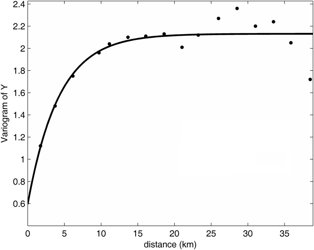
Variogram of the logarithmic transmissivities of the Land aquifer of Mostaganem: .
Variogramme de log T de la nappe du plateau de Mostaganem.
7.1 Case study
The routines involve:
- • estimating the omnidirectionnal variogram of the fitted log T field;
- • rescaling the parameters of the variogram to provide σY and lY to infer the optimum relaxation factor;
- • extrapolating the experimental curve ωopt via a preliminary fitting process;
- • taking into account the influence of the mesh size.
The value of ωopt obtained in this way is equal to 1.93, which is relatively different from the value of 1.85 obtained with experimental trials. This difference may be due to the inadequate characterization of Y, even if the experimental variogram can be fitted by an exponential function. Moreover, much of the uncertainty is induced by the extrapolation process.
8 Conclusion
The optimum value of the over-relaxation factor ω for the best convergence rate of SOR lies between 1 and 2 and is commonly between 1.6 and 1.9 (Trescott et al., 1980). In heterogeneous fields, this optimum over-relaxation factor should be chosen greater than the ones used in less heterogeneous fields.
The correlation length of Y, the log-tranmissivity field, strengthens this fact, since a short correlation length is symptomatic of a high heterogeneity and a long correlation length of a low heterogeneity. The standard deviation σY as well as the correlation length lY and the mesh spacing Δx appear as the controlling factors for estimating the over-relaxation coefficient.
According to the heuristic estimate used in Eq. (10), the optimal over-relaxation factor ωopt may be estimated by the expression:
| (22) |
- • the mesh size Δx′;
- • the standard-deviation σY; and
- • the correlation length lY of the distribution Y.
This expression is shown on Fig. 2 as a family of curves parameterized on lY for the particular case . A functional relationship expresses these curves as a polynomial of the 5th degree of the standard-deviation σY.
The reliability of SSOR and diagonal preconditioners were experimented for increasing values of the standard-deviation σY. SSOR is quite sensitive to ω but performs better than the other methods if a correct value of ω is chosen. The Jacobi method, although slightly less efficient, is quite robust with respect to increasing values of σY. An analysis of the spatial variability of Y can provide the parameters σY and lY which in turn will assign a narrow interval to infer reliability of ωopt from Fig. 3, for a given size of the mesh. Moreover, only the lower half interval was investigated since overestimates of ωopt, i.e. ωopt ≥ ω, have a lower negative impact on the efficiency of over-relaxation than underestimates. Then, in the spirit of equation (22), the following guidelines may be given to over-relax the heads with the SOR method: greater values of ωopt should be selected when:
- • the porous medium is more heterogeneous;
- • the Y-field is less correlated and;
- • the grid is finer.
Thus, a preliminary geostatistical study to evaluate the spatial variability of Y would be a convenient and judicious way to get a rough estimate of ωopt as it did to identify transmissivity (Roth et al., 1998). Therefore, it would be helpful to have an algorithm that assigns values to ωopt leading to an improved practical use of SOR either as an optimized solver or as a preconditioner for others iterative methods via a forward SOR sweep followed by a backward SOR sweep. Such an algorithm is relevant to expert systems and is presently beyond the state of the art in groundwater modelling. The case study showed here that relatively inexpensive rough geostatistical estimates of σYand lY can yield reasonable estimates for the optimal value of the over-relaxation factor ω. The above procedure, together with incorporating Latin Hypercube Sampling into existing Monte Carlo simulation software, can be extend to other iterative and optimisation methods. The formal investigation made here on the smoothing property of SOR suggests a promising way to improve both Gauss-Seidel and Jacobi smoothers.
Acknowledgments
The author wishes to express his gratitude to Pr Ghislain de Marsily, Dr. Patrick Goblet and an anonymous reviewer for their suggestions and comments on an earlier draft of this manuscript.