

1 Introduction
Global mean sea level (GMSL) change is a considerable interest variable in climate change studies. The measurement of changes in sea level can provide an important corroboration of predictions by climate models of global warming. For the past century, tide gauges show that global mean sea level rose at a rate of around 1.7 mm/year (Church and White, 2011). More recently and during the satellite era of sea level measurement (1993–2009), the rate of rise is estimated at around 3.2 ± 0.4 mm/year from the satellite data (Cazenave and Llovel, 2010; Church and White, 2011; Mitchum et al., 2010; Nerem et al., 2010) and 2.8 ± 0.8 mm/year from in-situ data (Church and White, 2011). This rate is significantly higher than the mean rate recorded by tide gauges over the past century.
The main factors causing current global mean sea level rise are thermal expansion of seawaters, land ice loss and water mass exchange between oceans and land water reservoirs. On average, over the satellite altimetry era (1993–2010), the contribution of ocean warming to the observed sea level rise is about 30% (Cazenave and Llovel, 2010; Cazenave and Remy, 2011; Church et al., 2011), while the contribution of glaciers and ice caps is accounted for ∼ 30% of sea level rise (Church et al., 2011; Cogley, 2009; Steffen et al., 2010). Although not constant through time, on average over 1993–2010, ice sheets mass loss explains ∼ 20% of the rate of sea level rise (Cazenave and Remy, 2011; Church et al., 2011; Steffen et al., 2010). A review of sea level evolution, globally and regionally, during the 20th century and the last two decades and the contributions to recent GMSL rise is given in Meyssignac and Cazenave (2012).
Recent studies have been aimed at explaining the influence of ENSO on the global mean sea level, which might result from changes in either global ocean heat content or global ocean mass. Considering the Multivariate ENSO Index (MEI) over 1993–2010, Nerem et al. (2010) noticed that detrended GMSL changes are correlated with ENSO occurrences, with positive/negative sea level anomalies observed during El Niño/La Niña events. Strong El Niño events have the potential to temporarily increase the global sea level (Cazenave et al., 2012; Ngo-Duc et al., 2005), whereas in the cold La Niña phase, the opposite occurs and sea level may exhibit a temporary fall.
Based on a global water mass conservation approach using GRACE satellite data and the (ISBA–TRIP) global hydrological model developed by Météo France (Alkama et al., 2010), Llovel et al. (2011) showed the close relationship between the interannual global mean sea level changes and land water storage variations, with a tendency for a deficit in land water storage during El Niño events, and vice versa during La Niña (with the Amazon basin as a dominant contributor to the latter).
Recent investigations suggest in addition that positive/negative mean sea level anomalies during El Niño/La Niña essentially result from positive/negative mass anomalies in the north tropical Pacific Ocean, possibly associated with reduced/increased transport of Pacific waters into the Indian Ocean through the Indonesian straits (Cazenave et al., 2012). Using a combination of GRACE satellite data and in-situ ocean temperature and rainfall data, Boening et al. (2012) show that during the 2011 strong La Niña event, the change in the sea level is due to water mass temporarily shifting from oceans to land as precipitation increased over Australia, northern South America, and Southeast Asia, while it decreased over the oceans. This study presents the first direct observation of the ENSO-induced exchange of freshwater that drives interannual changes in GMSL.
In this paper and at the first stage, we aim to provide a description of the global mean sea level variations. For this purpose, an unobserved components model (Young et al., 1999) based on a trend plus an auto-regression (AR) component is used to investigate homogeneous measurements of mean sea level anomalies datasets from the TOPEX and Jason series of satellite radar altimeters. The GMSL trend is extracted from the time series and a perturbational component about the trend is modelled as a pure AR component. Such an approach is useful in cases where the periodic behaviour of the perturbation about the trend is not very marked.
In the second stage, we investigate the impact of the ENSO phenomenon on the GMSL changes. For this, we considered the sea surface temperature anomalies (SSTA) index over the Niño3 region (5°N to 5°S, 150°W to 90°W). The cross wavelet transform and wavelet coherence analysis (Grinsted et al., 2004) are used for examining relationships in time-frequency space between the two time series of GMSL and SSTA.
The rest of the paper is organized as follows. Section 2 describes the two datasets used in this study. The two models used for trend extraction and for the coherence analysis are briefly explained in Section 3. Section 4 describes the application of UCM for GMSL time series analysis. The UCM model is used to interpolate the datasets over periods when measurements are missing and to decompose the time series into trend and harmonic components. Furthermore, this section uses the cross wavelet transform and wavelet coherence analysis to localize similarities in time and scale between the global mean sea level and Niño3 SSTA time series. The empirical results are addressed in this section. Section 5 concludes.
2 The data
2.1 Global mean sea level reference series
Radar altimeters permanently transmit signals to the Earth, and receive the reflected echo from the sea surface. The satellite orbit has to be accurately tracked and its position is determined relative to a reference surface (an ellipsoid). The sea surface height (SSH) is calculated by subtracting the measured distance between the satellite and sea surface from the precise orbit of the satellite. The sea level anomalies (SLA), defined as variations of the sea surface height (SSH) with respect to an a priori mean sea surface (MSS), are generally used as precious and main indicators for the development of scientific applications that aim to study the ocean variability (mesoscale circulation, seasonal variations, El Niño…).
In our research, we investigate a temporal series of averaged sea level anomalies (SLA) over all oceans and seas for the entire altimetry period, obtained by combining the time series from all three TOPEX, Jason-1 and Jason-2 missions (Nerem et al., 2010). These datasets were provided by the CU Sea Level Research Group of the University of Colorado1. This series covers the time period from the beginning of 1993 to the end of 2012 (20 years), with a sampling rate of 10 days.
The used mean sea level anomalies series is represented on Fig. 1. The main input data for computing this series are the Geophysical Data Records produced by NASA and CNES (TOPEX, Jason-1, Jason-2), which are therefore of the highest quality, notably in orbit determination. The three missions are linked together during the “verification” phases of the Jason-1 and Jason-2 missions in order to calculate very precisely the bias in GMSL between these missions. TOPEX and Jason-1 were connected by applying a bias of 88.48 mm to Jason-1's GMSL. Similarly, Jason-2's GMSL was connected to Jason-1's GMSL by applying a bias of 58.52 mm to Jason-2's GMSL and also by adding the bias between Jason-1 and TOPEX/Poseidon. All of the standard corrections to the altimeter range were applied to the sea surface height (SSH), including removal of ocean tides and an inverted barometer correction. The used mean sea surface (MSS) is the CLS01 model (Hernandez and Schaeffer, 2001), obtained from 7 years of TOPEX/Poseidon data, 5 years of ERS-1/2 data, 2 years of Geosat data added to ERS-1 geodetic data, which were processed and homogenized in order to produce a (1/30° × 1/30°) gridded map. Table 1 describes the parameters used by the University of Colorado for computing global mean sea level reference series.
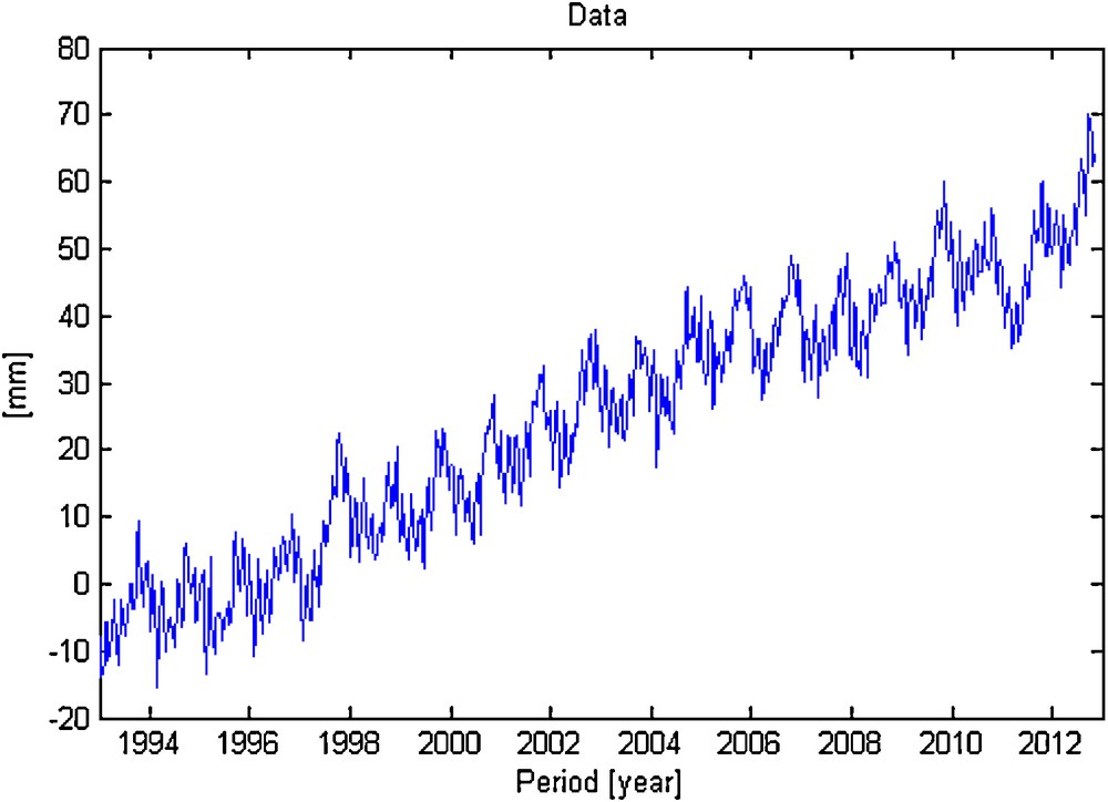
Global mean sea level anomalies time series (1993–2012).
Altimetry data processing parameters and corrections.
| Parameters | TOPEX | Jason-1 | Jason-2 |
| Time period | Dec. 06, 1992 to Jan. 10, 2002 | Jan. 15, 2002 to July 2, 2008 | July 3, 2008 to present |
| Cycles | 8–343 | 1–239 | 1–current |
| Base data set | MGDR-B | GDR-C | GDR-T |
| Orbit | STD0905 (Lemoine et al., 2010) | ||
| Range & corrections | |||
| Waveform tracker | GDR | ||
| Dry troposphere | GDR (from ECMWF) | ||
| Wet troposphere | TMR (Replacement Product v.1.0) | GDR-C (Cycles 1–227); JMR Replacement Product (Cycles 228–259) | AMR (GDR) |
| Ionosphere | GDR | ||
| Sea state bias | CLS Collinear v. 2009 (Tran et al., 2010) | ||
| Center of gravity | MGDR-B | N/A | |
| Mean sea surface & corrections | |||
| Mean sea surface | CLS01 (Hernandez and Schaeffer, 2001) | ||
| Ocean tide & loading tide | GOT4.7 (Ray, 1999) | ||
| Solid earth tide | GDR (Cartwright and Tayler, 1971; Cartwright and Edden, 1973) | ||
| Pole tide | GDR (Wahr, 1985) | ||
| Atmospheric pressure (inverted barometer) | AVISO dynamic atmosphere correction (DAC) that combines MOG2D high-frequency and inverted barometer low-frequency signals (Pascual et al., 2008) | ||
| Glacial isostatic adjustment (GIA) | −0.3 mm/year (Peltier, 2001, 2002, 2009; Peltier and Luthcke, 2009) | ||
| Processing corrections | |||
| Inter-mission bias | 88.48 mm (TOPEX to Jason-1) | 58.52 mm (Jason-1 to Jason-2) | |
| Minimum ocean depth | 120 m | ||
| Outlier removal | Anomaly greater than 2 m |
2.2 Sea surface temperature anomalies series
Monitoring of ENSO conditions primarily focuses on the sea surface temperature anomaly (SSTA) index (variations from an average or other statistical reference value) in the equatorial Pacific. SSTA equal to or greater than 0.5 °C in the Niño3 region (5°N to 5°S, 150°W to 90°W), or exceeding 0.4 °C in the Niño3.4 region (5°N to 5°S, 170°W to 120°W), could indicate ENSO warm phase (El Niño) conditions (Trenberth, 1997), while anomalies less than or equal to −0.5 °C (or −0.4 °C for the Niño3.4 region) are associated with cool phase (La Niña) conditions.
In this paper, the used ENSO index was the average of SSTA computed over the Niño3 region (5°S to 5°N, 90°W to 150°W), with respect to a 1971–2000 month climatology (Xue et al., 2003). These data sets were obtained from the most recent version (v3b) of the NCDC Extended Reconstruction Sea Surface Temperatures (ERSST) analysis2, monthly from January 1880 to June 2010. ERSST.v3b was generated using in-situ Sea Surface Temperature (SST) data and improved statistical methods that allow stable reconstruction using sparse data. The monthly analysis extends from January 1854 to the present, but because of sparse data in the early years, the analyzed signal was damped before 1880. After 1880, the strength of the signal was more consistent over time. ERSST is suitable for long-term global and basin wide studies; local and short-term variations have been smoothed in ERSST. The ERSST.v3b analysis is exactly as described in the ERSST.v3 paper (Smith et al., 2008), with one exception: satellite SST data are not used in ERSST.v3b.
3 Methodology
3.1 The unobserved components model (UCM)
The UCM are models in which time series are decomposed as the sum or a product of a number of other simple time series with economic or physical meaning. One widely accepted univariate version of UCM is (Young et al., 1999):
| (1) |
In practice, not all the components in eq. (1) are necessary: indeed, the simultaneous presence of all these components can induce identification problems and so use of the complete model (1) is not advisable in practice unless adequate precautions are taken. In this paper, the simplified used model is one such decomposition that contains only the trend plus an AR component, seasonal and white noise components.
The trend component is formulated in a stochastic state space context and then solved by using an integrated random walk (IRW) plus noise modelling approach. The full state space description is given by the state equation (Pedregal and Trapero, 2007):
| (2) |
| (3) |
x1t is the first state variable known as the ‘level’, x2t is the second state variable and generally known as the ‘slope’, ηt is a zero mean, serially uncorrelated white noise process with a certain variance. Young et al. (1999, 2007) also defined two parameters for computing convenience: noise variance ratio (NVR) Qr and . Qr is a normalized matrix of the diagonal noise variance matrix Q, and is the error covariance matrix associated with the estimation state. Young et al. (1999) propose one final simplification using the estimate of the trend from an autoregressive (AR) model. The AR order is identified by the Akaike's Information Criterion (AIC), whereas, the seasonal term is modelled as a sum of the fundamental signal and of its associated harmonics:
| (4) |
3.2 Cross wavelet transform and wavelet coherence
The cross wavelet transform and wavelet coherence analysis used in this paper follows the method of Grinsted et al. (2004). Although the basic components of this analysis are reviewed here, readers are referred to Grinsted et al. (2004) for a more detailed explanation.
The continuous wavelet transform (CWT) allows analyzing the temporal evolution of the frequency content of a given signal or timing series. The CWT of a time series (xn, n = 1, …, N), with uniform time steps δt, is defined as the convolution of xn with the scaled and normalized wavelet:
| (5) |
The wavelet power is defined as . The complex argument of can be interpreted as the local phase (Torrence and Compo, 1998).
From two CWTs we construct the cross wavelet transform (XWT), which will expose their common power and relative phase in time–frequency space. The XWT of two time series xn and yn is defined as:
| (6) |
Following Torrence and Webster (1999), the wavelet coherence (WTC) of two time series, which can find significant coherence even though the common power is low, is defined as:
| (7) |
4 Results and discussion
4.1 Global mean sea level reference series analysis
All of the results in this section are obtained by means of the Captain Toolbox v7.53 (Taylor et al., 2007). The Captain Toolbox is a set of MATLAB functions for non-stationary time series analysis and forecasting. It allows the identification of unobserved components models, time variable parameter models, state-dependent parameter models and multiple-input discrete and continuous time-transfer function models. The toolbox is useful for system identification, signal extraction, interpolation, backcasting, forecasting and databased mechanistic analysis of a wide range of linear and nonlinear stochastic systems.
The global mean sea level series was decomposed into trend and seasonal components using a model based on a trend plus an AR component. Apart from the decomposition of time series into trend and seasonal components, this methodology also provides a time series model of the data, which is used for the interpolation of missing data. Note that this model can also be used for backcasting and forecasting.
In the first place, we estimated a smooth trend using an IRW with an initial noise variance ratio (NVR) hyper-parameter of 10−4. The green line and the red line on Fig. 2 correspond to the smooth trend and the residuals series, respectively.

Smooth trend using an integrated random walk with an initial noise variance ratio hyper-parameter of 1 × 10⁻⁴.
Then, the order of the autoregressive (AR) model for the perturbations is identified using the AIC. We searched for models ranging from 1st to the 10th order. The best-fit AR polynomial is obtained for an order of 9. The AR model for the perturbations is estimated, together with the associated optimal NVR for the IRW trend.
Table 2 represents the estimation results of the perturbational component about the trend, were P is the AR order for perturbations, ARp is the AR polynomials for the perturbations and ARpse is the standard error of AR parameters for perturbations.
AR model for perturbations.
| P | ARp | ARpse |
| 1 | −0.6999 | 0.0376 |
| 2 | 0.2256 | 0.0460 |
| 3 | −0.0731 | 0.0464 |
| 4 | −0.1440 | 0.0464 |
| 5 | −0.2162 | 0.0459 |
| 6 | −0.0995 | 0.0464 |
| 7 | 0.1631 | 0.0465 |
| 8 | 0.0605 | 0.0462 |
| 9 | 0.1918 | 0.0376 |
The final trend NVR is estimated at 2.7554 × 10⁻⁴, with a trend integration order of 2. Finally, both components (trend and seasonal component) are estimated simultaneously.
Figs. 3, 4 and 5 represent the estimated trend, the total seasonal component and the fitted data, respectively. A zoom on the final 2 years, with the standard errors, is shown on Fig. 6.
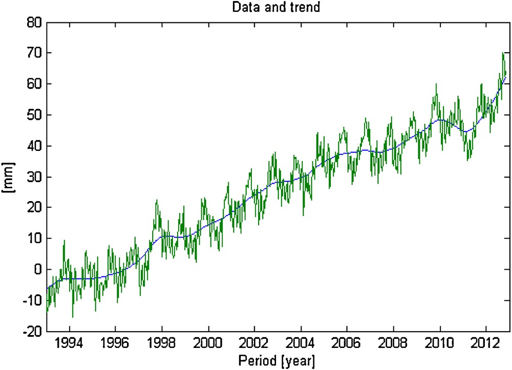
Global mean sea level anomalies time series and estimated trend (1993–2012).
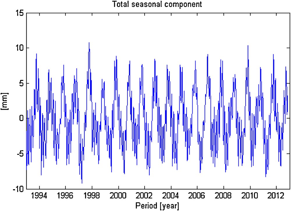
Estimated total seasonal component.

Global mean sea level anomalies time series (blue line), fit model (green line) and residuals (red line).
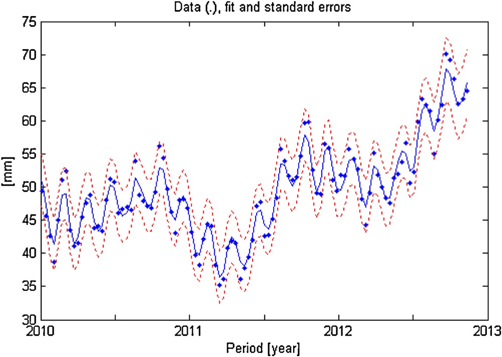
Data, fit and standard errors of the final 3 years.
The analysis of the estimated trend indicates that the global mean sea level is subject to significant rise, from −6 mm to 62 mm during the period 1993–2012. Applying a least squares linear regression analysis to the extracted trend gives a rate of 3.22 mm/year between 1993 and 2012, with a formal error of 0.02 mm/year (see Fig. 7).

Estimated trend and linear regression line.
The estimated rate of GMSL rise agrees with the CU GMSL rate4 over the same period of 3.2 ± 0.4 mm/year, where the realistic error assigned in this quantity (± 0.4 mm/year) is based on comparisons of altimeter heights with tide gauge-based sea level measurements (Mitchum, 2000). For further information on errors assessment affecting the calculation of the GMSL rate and comparison of altimetry-based sea level with in-situ measurements, the reader is referred to Ablain et al. (2009).
One can see on Fig. 7 evidence that there are a number of fluctuations over short periods in the estimated trend. This variability is at least partly related to El Niño/La Niña episodes (sea level rises during El Niño and falls during La Niña) and associated changes in the hydrological cycle.
4.2 Correlation between global mean sea level variability and El Niño-southern oscillation
To compare the global mean sea level to the sea surface temperature anomalies index over the Niño3 region, we removed from original global mean sea level time series (series of mean sea level anomalies) the extracted trend and the total seasonal components (both estimated in Section 4.1). Then, since ERSST.v3b SSTA data are monthly distributed, we created from the detrended GMSL datasets a lower resolution series with a time scale of one month to be used for relationship analysis.
Fig. 8 shows the used averaged SSTA time series (1993–2012) over the Niño3 region and the detrended and seasonally adjusted GMSL series used for correlation analysis. The plotted series show a strong correlation between the global mean sea level and the SSTA Niño3 index.
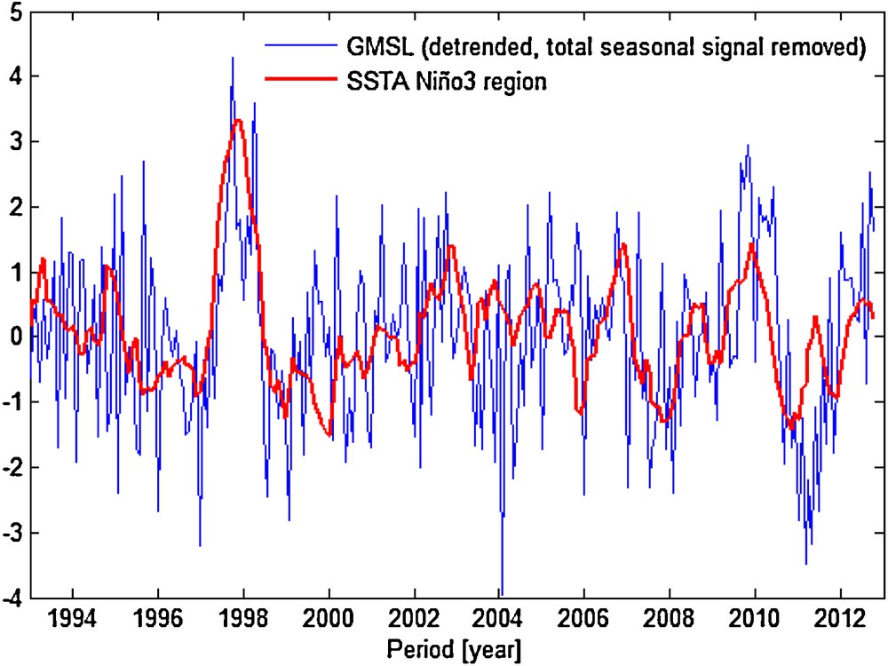
Global mean sea level (detrended and total seasonal component removed) series and mean sea surface temperature anomalies series over the Niño3 region.
One can see from Fig. 8 evidence that there was a particularly strong warm event of large amplitude during the 1997–1998 period. The El Niño of 1997–98 was extremely severe. This event was a so-called “Type-1” El Niño (Fu et al., 1986), having the strongest averaged SSTA > 3.0 °C from October 1997 to January 1998 (see Fig. 8). Although it started in April to May 1997, its effects extended into the early summer of 1998.
In early 2006, sea surface temperature positive anomalies are measured in the central equatorial Pacific. These high-temperature anomalies characterize a new El Niño event. In early summer 2009, sea surface height positive anomalies are measured from August 2009, with a maximum during November 2009 (SSTA > 1.1 °C), characterizing a moderate El Niño event (see Fig. 8).
Severe La Niña was also formed in 1998 and 2012. From June 2007, data indicated a moderate La Niña event, which strengthened until early 2008. A new La Niña episode was developed in mid-2010, and lasted until early 2011. It intensified again in the mid-2011 (see Fig. 7). Between the beginning of 2010 and the middle of 2011, sea level fell until −3 mm. This occurred concurrently with the strong phase, La Niña 2011.
For examining strictly speaking relationships between the two time series SSTA and GMSL (detrended and total seasonal component removed) series in time–frequency space, first the CWT of both datasets was calculated. The XWT and WTC tests are then performed.
The CWT of the SSTA index and GMSL series are shown on Fig. 9. There are clearly common features in the wavelet power of the two time series in the 2–4-year band in the period from 1996 to 2000. However, the similarity between the two patterns for other periods is quite low and it is therefore hard to say whether it is significant. The cross wavelet transform helps in this regard; it will expose the common power and relative phase in the time-frequency space.
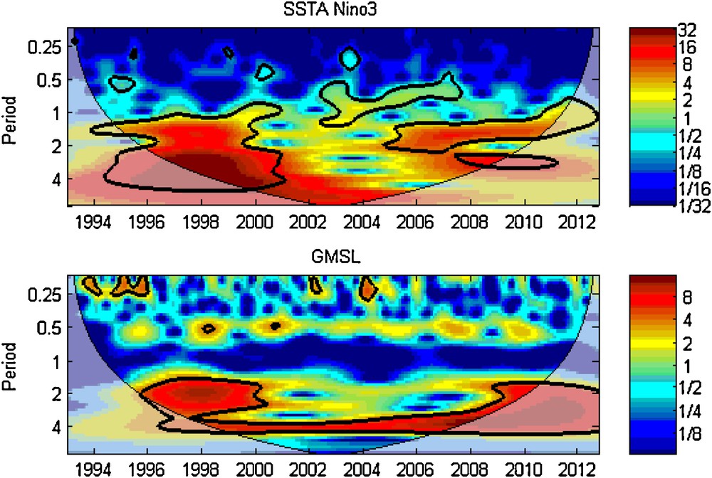
Continuous wavelet power spectrum of global mean sea level time series (top) and mean sea surface temperature anomalies series over the Niño3 region (bottom). The thick black contour designates the 5% significance level against red noise, and the cone of influence where edge effects might distort the picture is shown as a lighter shade.
The XWT of SSTA index and GMSL and their relative phase relationship (with in-phase: arrows pointing right, anti-phase: arrows pointing left) are shown on Fig. 10. Here we note that there is a significant common power in the 1–4-year band from 1996 to 2000. Also, there is an appreciable power in the 1–2-year band from 2005–2010. All these areas show an in-phase relationship, suggesting that GMSL and SSTA vary synchronously.
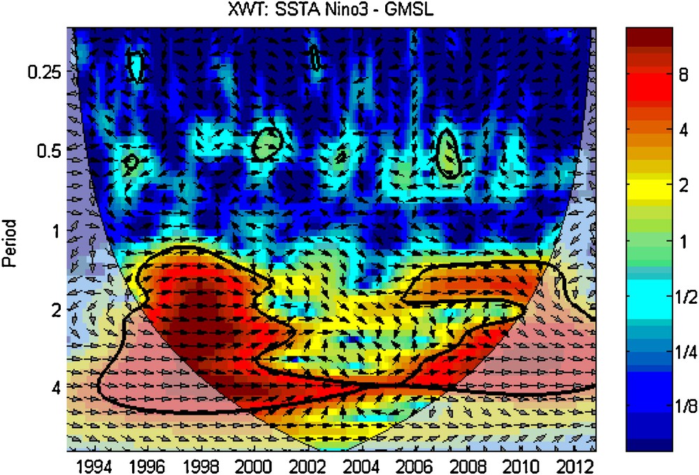
Cross wavelet transform of global mean sea level and sea surface temperature anomalies series. The 5% significance level against the red noise is shown as a thick contour. The relative phase relationship is shown as arrows (with in-phase pointing right, anti-phase pointing left).
The squared WTC of SSTA and GMSL is shown on Fig. 11. Compared with the XWT, a larger section stands out as being significant and all these areas show an in-phase relationship between SSTA and GMSL. Oscillations in SSTA are manifested in the GMSL on wavelengths varying from 1–4 years in the period from 1996 to 2000 (El Niño 1997–98), 1–2 years in the period from 2005 to 2008 (2006–2007 El Niño event and 2007–2008 La Niña episode). Also, there is an appreciable section in the 3–4-year band from 2007–2012 (2009–2010 El Niño, 2010–2011 La Niña events), though this area is outside of the cone of influence in which edge effects are considerable.
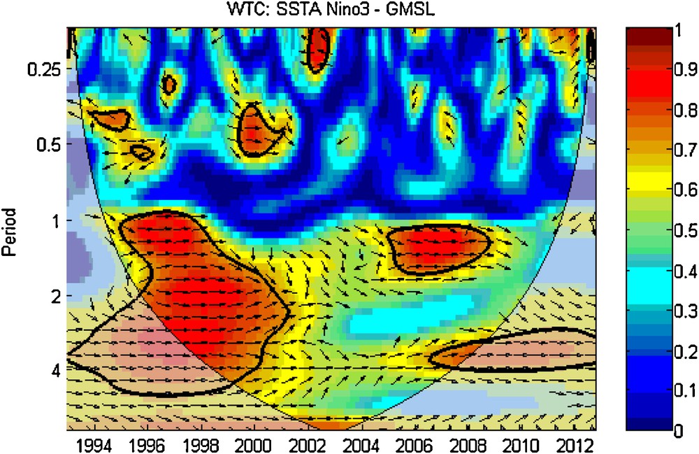
Squared wavelet coherence between the sea surface temperature anomalies and global mean sea level time series. The 5% significance level against the red noise is shown as a thick contour. All significant sections show in-phase behavior.
5 Conclusions
In this paper, an approach of seasonal adjustment and trend extraction based on the unobserved components model (UCM) has been used to investigate the global mean sea level anomalies (GSLA) series. Our GMSL trend gives a rate of 3.22 ± 0.4 mm/year between 1993 and 2012. This obtained rate agrees with the study of the CU Sea Level Research Group, which suggested a sea level rise rate of 3.2 ± 0.4 mm/year over the same period. Although the extracted global trend indicates a rise in the mean level of the oceans, there are marked fluctuations over short periods.
Cross wavelet transform and wavelet coherence analysis were successfully employed to expose common power between the GMSL changes and ENSO episodes and their relative phase in time–frequency space. The results indicate a correlation between GMSL changes and ENSO episodes on wavelengths band of 1–4 years in the period from 1996 to 2000, 1–2 years in the period from 2005 to 2008 and also in the 3–4-year band from 2007–2012. This is a pertinent result of a high correlation between the GMSL variability and El Niño/La Niña episodes.
Acknowledgments
We are very grateful to the Colorado Center for Astrodynamics Research of the University of Colorado, Boulder, and the National Climatic Data Center (NCDC) for providing global mean sea level time series and ERSST.v3b SSTA data, respectively. We also thank the Centre for Research on Environmental Systems (CRES) of the Lancaster University for providing the Captain toolbox. We are enormously grateful to Anny Cazenave (LEGOS–CNES) for helpful comments and suggestions that helped us to improve our manuscript.