Seismic random noise attenuation by time-frequency peak filtering based on joint time-frequency distribution

Chao Zhang; Hong-bo Lin; Yue Li; Bao-jun Yang

doi:10.1016/j.crte.2013.07.005

Internal geophysics

Seismic random noise attenuation by time-frequency peak filtering based on joint time-frequency distribution

Chao Zhang ¹ ; Hong-bo Lin ¹ ; Yue Li ¹ ; Bao-jun Yang ²

¹ College of Communication Engineering, Department of Information Engineering, Jilin University, No. 5372 Nanhu Road, Changchun, Jilin 130012, China
² Department of Geophysics, Jilin University, Changchun 130026, China

Comptes Rendus. Géoscience, Volume 345 (2013) no. 9-10, pp. 383-391.

Résumé

Time-Frequency Peak Filtering (TFPF) is an effective method to eliminate pervasive random noise when seismic signals are analyzed. In conventional TFPF, the pseudo Wigner–Ville distribution (PWVD) is used for estimating instantaneous frequency (IF), but is sensitive to noise interferences that mask the borderline between signal and noise and detract the energy concentration on the IF curve. This leads to the deviation of the peaks of the pseudo Wigner–Ville distribution from the instantaneous frequency, which is the cause of undesirable lateral oscillations as well as of amplitude attenuation of the highly varying seismic signal, and ultimately of the biased seismic signal. With the purpose to overcome greatly these drawbacks and increase the signal-to-noise ratio, we propose in this paper a TFPF refinement that is based upon the joint time-frequency distribution (JTFD). The joint time-frequency distribution is obtained by the combination of the PWVD and smooth PWVD (SPWVD). First we use SPWVD to generate a broad time-frequency area of the signal. Then this area is filtered with a step function to remove some divergent time-frequency points. Finally, the joint time-frequency distribution JTFD is obtained from PWVD weighted by this filtered distribution. The objective pursued with all these operations is to reduce the effects of the interferences and enhance the energy concentration around the IF of the signal in the time-frequency domain. Experiments with synthetic and real seismic data demonstrate that TFPF based on the joint time-frequency distribution can effectively suppress strong random noise and preserve events of interest.

Métadonnées

Reçu le : 2013-07-04
Accepté le : 2013-07-31
Publié le : 2013-09-01

DOI : 10.1016/j.crte.2013.07.005

Mots clés : Time-Frequency Peak Filtering, Pseudo Wigner–Ville Distribution, Smoothed Pseudo Wigner–Ville Distribution, Signal-to-Noise Ratio, Denoising

Affiliations des auteurs :

Chao Zhang ¹ ; Hong-bo Lin ¹ ; Yue Li ¹ ; Bao-jun Yang ²

@article{CRGEOS_2013__345_9-10_383_0,
     author = {Chao Zhang and Hong-bo Lin and Yue Li and Bao-jun Yang},
     title = {Seismic random noise attenuation by time-frequency peak filtering based on joint time-frequency distribution},
     journal = {Comptes Rendus. G\'eoscience},
     pages = {383--391},
     publisher = {Elsevier},
     volume = {345},
     number = {9-10},
     year = {2013},
     doi = {10.1016/j.crte.2013.07.005},
     language = {en},
}

TY  - JOUR
AU  - Chao Zhang
AU  - Hong-bo Lin
AU  - Yue Li
AU  - Bao-jun Yang
TI  - Seismic random noise attenuation by time-frequency peak filtering based on joint time-frequency distribution
JO  - Comptes Rendus. Géoscience
PY  - 2013
SP  - 383
EP  - 391
VL  - 345
IS  - 9-10
PB  - Elsevier
DO  - 10.1016/j.crte.2013.07.005
LA  - en
ID  - CRGEOS_2013__345_9-10_383_0
ER  -

%0 Journal Article
%A Chao Zhang
%A Hong-bo Lin
%A Yue Li
%A Bao-jun Yang
%T Seismic random noise attenuation by time-frequency peak filtering based on joint time-frequency distribution
%J Comptes Rendus. Géoscience
%D 2013
%P 383-391
%V 345
%N 9-10
%I Elsevier
%R 10.1016/j.crte.2013.07.005
%G en
%F CRGEOS_2013__345_9-10_383_0

Chao Zhang; Hong-bo Lin; Yue Li; Bao-jun Yang. Seismic random noise attenuation by time-frequency peak filtering based on joint time-frequency distribution. Comptes Rendus. Géoscience, Volume 345 (2013) no. 9-10, pp. 383-391. doi : 10.1016/j.crte.2013.07.005. https://comptes-rendus.academie-sciences.fr/geoscience/articles/10.1016/j.crte.2013.07.005/

Version originale du texte intégral

1 Introduction

Field seismic data contain a significant amount of noise which has a strong interference on the signal for seismic exploration. Noise elimination is a very important step in seismic data processing (Zhang and Klemperer, 2005). Unlike coherent noise, random noise is unpredictable and incoherent in space and time. Abundant methods coming from different fields have been proposed for seismic random noise attenuation, such as median filtering (Duncan and Beresford, 1995), frequency-spatial prediction (Wang, 1999, 2002), wavelet transform (Cao and Chen, 2005), polynomial approximation (Lu et al., 2006), singular value decomposition (Lu, 2006) and so on. However, most of the existing methods have a negative effect on denoising in the case of low signal-to-noise ratio (SNR). It may cause attenuation of useful signals and therefore hinder the seismic data processing. Hence, one of the tasks in the seismic data processing is to design a useful denoising method to eliminate the random noise as much as possible, but at the same time able to preserve or recover the important features in the cases of low SNR.

Time-frequency peak filtering (TFPF) can give an unbiased estimation of the signal in cases where it is linear in time and contaminated by stationary white Gaussian noise (Barkat and Boashash, 1999; Boashash and Mesbah, 2004; Zahir and Hussain, 2000), and is a technique successfully applied to seismic signal processing (Lin et al., 2007; Wu et al., 2011). Conventional TFPF is generally biased when the pseudo Wigner–Ville distribution (PWVD) is used to estimate instantaneous frequency of the analytic signal. The smoothing effect in the frequency domain results in a poor time-frequency concentration of PWVD. That means a deficient energy concentration on the curve of instantaneous frequency. Therefore, conventional TFPF based on PWVD cannot accomplish a very clean recovery of the original signal when SNR is indeed low.

In this paper, we focus on finding an ideal time-frequency distribution to enhance the energy concentration on the curve of the instantaneous frequency. In this way, we can reduce the bias in TFPF and achieve a greater denoising performance. We introduce a new joint time-frequency distribution (JTFD) to be applied to TFPF. This new distribution can be briefly named by its acronym JTFD. JTFD presents a double advantage: it gives rise to a higher concentration of the signal around its IF in time-frequency, and encloses a better ability to remove undesirable noise interferences. TFPF based on JTFD may further reduce random noise affecting the seismic data than conventional TFPF.

2 Time-frequency peak filtering

TFPF allows the attenuation of seismic noise by encoding the noisy seismic signal as the instantaneous frequency (IF) of the analytic signal. Assuming that the time-frequency distribution energy of the analytic signal is concentrated around the IF, we can estimate the instantaneous frequency on the analytic signal by means of the peak of the time-frequency distribution to recover the desired signal.

A seismic trace can be modeled by the following equation:

s (t) = x (t) + n (t)

(1)

where x(t) is the signal of interest and n(t) is the random noise. The fundamental problem consists of recovering the signal x(t) from the observed signal s(t). TFPF extracts the desired signal in two steps. First we encode the noisy signal s(t) by the IF of the analytic signal z(t) via frequency modulation. The z(t) function is expressed as:

z (t) = e^{j 2 π μ \int_{0}^{t} s (λ) d λ}

(2)

where μ is a scaling parameter analogous to a frequency modulation index. Then we calculate the PWVD of the analytic signal z(t), as defined by Barbarossa (1997):

P W V D_{z} (t, f) = \int_{- \infty}^{\infty} h (τ) z (t + τ / 2) z^{*} (t - τ / 2) e^{- j 2 π f τ} d τ

(3)

where h(τ) is a window function sliding with time. In the case where the PWVD peak is located at the IF, we take the peak frequency of the PWVD to obtain the estimated signal. It is expressed as:

\hat{x} (t) = \arg \max_{f} [PWVD (t, f)] / μ

(4)

In the conventional TFPF above, we use the PWVD for IF estimation. However, the time-frequency energy of the PWVD in the frequency direction is divergent and it is sensitive to noise interferences that mask the borderline between signal and noise in the time-frequency analysis. In other words, the interferences are the cause by which the peak of PWVD deviates from IF. Hence, this requires the appropriate adjustments in the time-frequency domain to enhance the energy concentration around the IF. To this end, we use the joint time-frequency distribution for filtering, which not only makes the energy of the signal become concentrated on the IF of each component, but also removes the interferences and enables the IF curve be readily identified.

3 Smoothed and filtered PWVD

The smoothed PWVD, hereafter denoted by SPWVD, is a time-frequency distribution that allows us to distinguish the borderline between signal and noise in time-frequency analysis, in such a way that the IF curve can be identified with clarity. The definition of SPWVD is (Auger and Flandrin, 1995):

{SPWVD}_{z} (t, f) = \int_{- \infty}^{+ \infty} \int_{- \infty}^{+ \infty} g (u) h (τ) z (t - u + τ / 2) z^{*} (t - u - τ / 2) e^{- j 2 f π τ} d u d τ

(5)

where h(τ) and g(u) are window functions with odd length, and g(0) = h(0) = 1. As smoothing is done in both time and frequency domains, SPWVD can largely eliminate noise interferences. Since the length of the two window functions can be controlled arbitrarily and independently, SPWVD allows one to adjust the window length adaptively in the process of suppressing noise interferences.

As an example, we start from the Ricker wavelet:

x (t) = (1 - 2 π^{2} f_{d}^{2} t^{2}) \exp (- π^{2} f_{d}^{2} t^{2})

(6)

where f_d is the dominant frequency.

The PWVD and SPWVD of a Ricker wavelet highly contaminated by additive white Gaussian noise (SNR = –10 dB) are shown in Fig. 1. The peak of PWVD deviates from IF because of the noise interferences. It is difficult to identify the IF curve in the PWVD as shown in Fig. 1a. As can be seen in Fig. 1b, the energy of the IF curve in the SPWVD is divergent. However, the IF curve can be recognized after smoothing in time and frequency. Hence, we plan to make use of SPWVD to get a broad distribution area of the IF curve.

Fig. 1
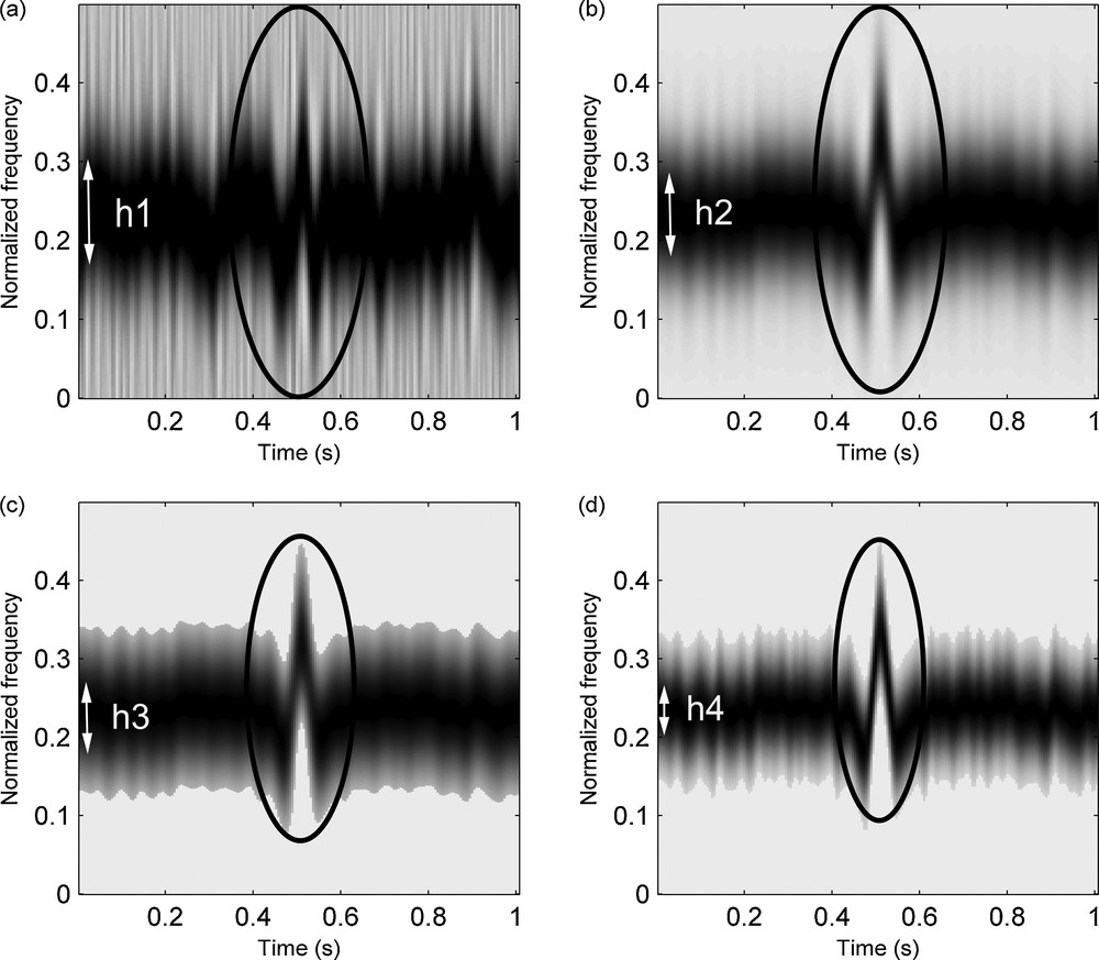
Comparison of different time-frequency distributions obtained from a Ricker wavelet contaminated by additive white Gaussian noise (SNR = –10 dB): (a) pseudo Wigner–Ville distribution (PWVD); (b) SPWVD smoothed distribution (after a double windowing in time and frequency); (c) SPWVD filtered distribution (processed by a step function); (d) JTFD weighted distribution (PWVD after being finally weighted by the previous filtered distribution). The notation h1,…, h4 indicates the width of each function (concentration of energy), while the ellipses enclose waveforms (evident accumulation of energy) in each case.

Due to the smoothing effect in the time-frequency domain, the time-frequency resolution of SPWVD decreases (Ghias et al., 2007). In order to remove divergent time-frequency points and make the IF curve clearer, the matrix SPWVD (t, f) is filtered with a step function. This non-linear filter has an input-output relation of the form:

SP \hat{W} VD (t, f) = \{\begin{cases} SPWVD (t, f), |SPWVD (t, f)| \geq T h (t), \\ 0, |SPWVD (t, f)| < T h (t) \end{cases}

(7)

where Th(t) is a time-varying threshold, whose expression is:

T h (t) = c_{1} \times \max (|SPWVD (t, f)|), c_{1} \in (0,1)

(8)

where c₁ is an adjustment coefficient whose value varies according to the noise level. When the noise level is very high, the threshold must be appropriate to eliminate noise interference. So the value of c₁ is selected as the normalized standard deviation of the signal to be processed, thus realizing an adaptive adjustment of the threshold under different noise levels.

The $SP \hat{W} VD (t, f)$ of the Ricker wavelet is shown in Fig. 1c. We can see that the time-frequency area of the signal is more effective and the noise interference is further suppressed. In this distribution matrix, the value of the IF curve is much higher than the noise interference. So we use $SP \hat{W} VD (t, f)$ to weight the PWVD of the signal in order to reduce the effects of the interferences and enhance the time-frequency concentration of the signal around IF.

4 Joint time-frequency distribution JTFD

The joint time-frequency distribution, hereafter denoted by JTFD, is a combination of PWVD and SPWVD. The whole weighting procedure can be expressed as follows:

JTFD (t, f) = PWVD (t, f) • SP \hat{W} VD (t, f)

(9)

where JTFD (t,f) denotes the matrix of the joint time-frequency distribution. The symbol • denotes scalar multiplication. The JTFD of the Ricker wavelet is shown in Fig. 1d. Through the contrast, we can see that the width of h4 is the narrowest, which means that the energy tends to be concentrated. Furthermore, the waveform enclosed in the ellipse in Fig. 1d is clearer due to energy accumulation. Therefore, JTFD not only allows the IF curve to be identified easily in the time-frequency domain, but also increases the concentration of the signal around its IF.

To further demonstrate the advantages of JTFD, we take again the Ricker wavelet. The dominant frequency of the wavelet is 25 Hz. Then we add white Gaussian noise (SNR = 0 dB) to the original wavelet. The amplitude spectra of PWVD, SPWVD and JTFD are shown in Fig. 2. The PWVD curve still reveals the energy fluctuations in the non-instantaneous frequency because of the noise interference, which results in some energy divergence, while the JTFD curve shows maximum amplitude in the instantaneous frequency and the energy here is higher than in the other two distributions. The JTFD amplitude for other frequencies is near to zero, so that JTFD makes the signal energy concentrated in the vicinity of the instantaneous frequency. In this way, we achieve a more accurate estimation of the instantaneous frequency by increasing the energy concentration in time-frequency and eliminating the interferences.

Fig. 2
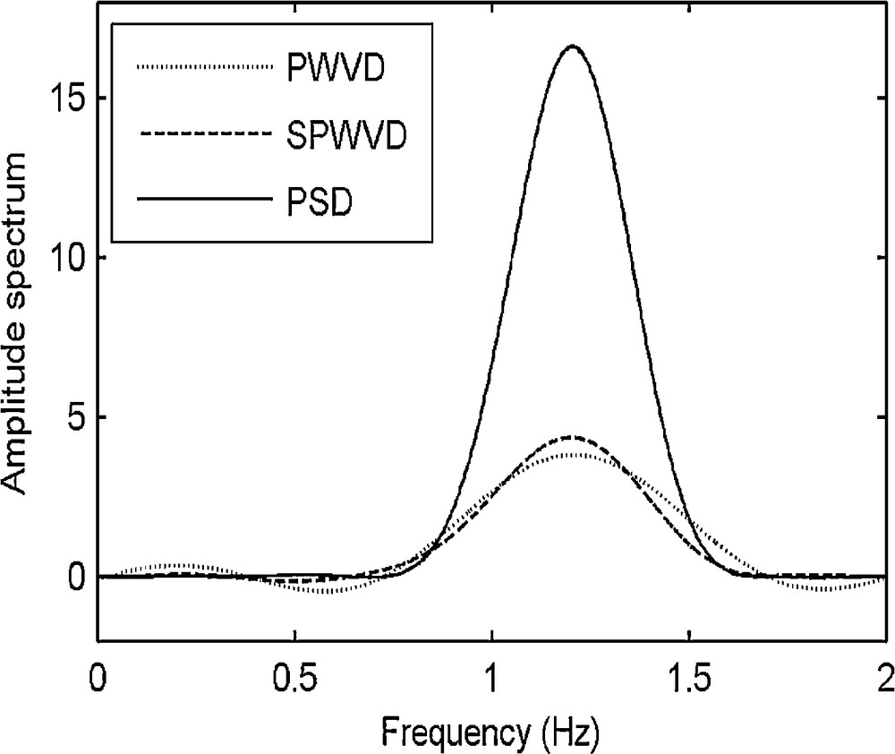
Starting from a Ricker wavelet of dominant frequency 25 Hz, with added white Gaussian noise (SNR = 0 dB), amplitude spectra of PWVD, SPWVD and JTFD.

5 Denoising with synthetic seismic data

JTFD is used for IF estimation to improve the drawbacks in conventional TFPF. To check the effectiveness of the modified TFPF, we present the following examples with synthetic seismic data. The first case is a seismic model with two cross-events, as shown in Fig. 3a. The dominant frequencies of the two events are 20 and 25 Hz. The source wavelet that we applied to simulate the waveform is a Ricker wavelet. In order to deal with more realistic synthetic data, we have added white Gauss noise to our synthetic data. Fig. 3b is a noisy version (SNR = –10 dB) of the noise-free representation in Fig. 3a. Modified TFPF is compared with conventional TFPF. Fig. 3c, d show the results obtained by both methods. Qualitatively, at a glance, we can get an idea of the achieved performance. The conventional TFPF can suppress some amount of random noise, but the effect is not fairly, while with the modified TFPF a larger amount of noise has been removed and the events are more clearly recovered.

Fig. 3
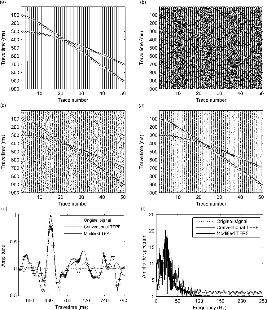
Denoising with synthetic seismic data: (a) Synthetic seismic data. Two Ricker wavelets of dominant frequencies 20 Hz and 25 Hz were considered to simulate synthetic waveforms as natural events; (b) noisy seismic data (SNR = –10 dB). The synthetic data were contaminated with white Gaussian noise; (c) result after applying conventional TFPF; (d) result after applying modified TFPF; (e) comparison of results after processing a single synthetic trace (18th trace) with both filtering types for noise suppression; (f) amplitude spectra of the original signal and the two filtered signals.

We can achieve a more detailed knowledge by analyzing a single trace and its amplitude spectrum. To this end, we extract the 18th trace of the synthetic records. The amplitudes of the waveforms in the time and frequency domains are shown in Fig. 3e, f. Fig. 3e exhibits the denoising result of seismic wavelet from the 18th trace of the synthetic record in time domain. Notice that the filtering result of modified TFPF is closer to the original signal and the amplitude value of noise on both sides of the signal is significantly lower than conventional TFPF does. The comparison in frequency domain is shown in Fig. 3f. We can see that the filtered signal spectrum of the modified method is more close to that of the original signal, and the amplitude spectrum of the signal in high frequency components beyond 100 Hz is approximately zero. So the random noise is better suppressed.

In the following, we check the effectiveness of the modified TFPF on SNR (in dB) and MSE after adding different levels of white Gaussian noise. The signal-to-noise ratio SNR and the mean square error MSE are calculated as follows:

SNR (dB) = 10 \times \log_{10} (P_{s} / P_{n})

(10)

MSE = \sqrt{N^{- 1} {\sum_{n} [\hat{x} (n) - x (n)]}^{2}}

(11)

where P_s is the power of original data and P_n is the power of noise. N denotes the number of wavelet samples;

\hat{x} (n)

denotes the estimated value of the signal, and x(n) is the true value.

The resulting SNR and MSE for synthetic seismic data (Fig. 3a) are given in Tables 1 and 2. The larger the SNR value and the lower the MSE value, the better the ﬁltering effects. Figs. 4 and 5 represent curves of SNR and MSE drawn from Tables 1 and 2. As can be seen in Figs. 4 and 5, the modified TFPF has obvious advantages when the SNR is below –10 dB. The SNRs after filtering by modified TFPF are larger and the MSEs are smaller than when applying conventional TFPF. The modified TFPF leads to a noticeably cleaner signal and more accurate estimations.

SNR (in dB) computed from the original signal	SNR (in dB) computed from the processed signal by conventional TFPF	SNR (in dB) computed from the processed signal by modified TFPF
–20	–13.36	–10.60
–16	–9.45	–6.61
–12	–5.41	–2.67
–8	–1.26	1.09
–4	2.34	4.64
0	5.56	7.62
4	8.05	9.82
8	9.73	11.24

SNR (in dB) computed from the original signal	MSE computed from the processed signal by conventional TFPF	MSE computed from the processed signal by modified TFPF
–20	0.5384	0.3915
–16	0.3407	0.2520
–12	0.2135	0.1617
–8	0.1359	0.1045
–4	0.0878	0.0699
0	0.0603	0.0488
4	0.0454	0.0373
8	0.0379	0.0315

Fig. 4
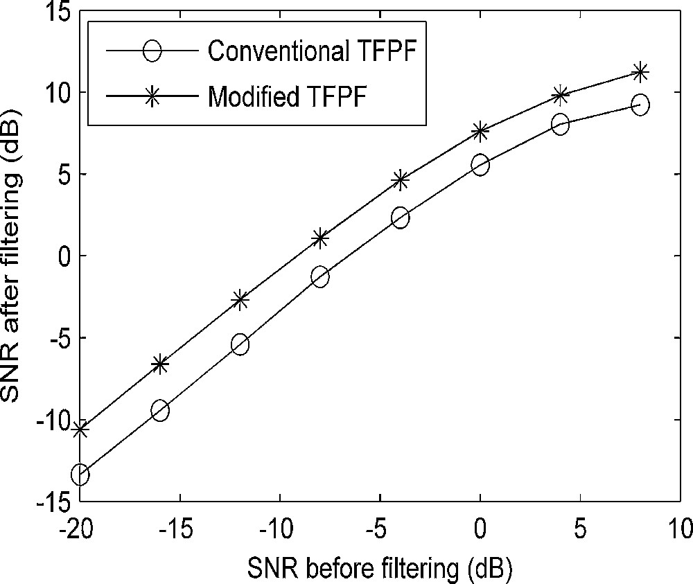
SNR curves obtained from the two denoising methods (Table 1) versus SNR before filtering. The values correspond to different noise levels.

Fig. 5
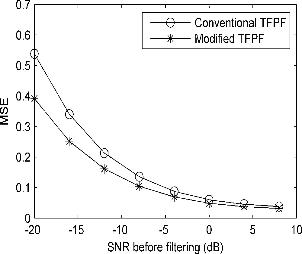
MSE curves obtained from the two denoising methods (Table 2) versus SNR before filtering. The values correspond to different noise levels.

The second example consists of a more complex model with four hyperbolic reflection events, as shown in Fig. 6a. Four Ricker wavelets of dominant frequencies 25 Hz, 30 Hz, 35 Hz and 40 Hz were used to simulate synthetic waveforms as natural events. As before, we have added white Gauss noise to the synthetic model. The noisy record with SNR = –15 dB is shown in Fig. 6b; in this illustration, the events are almost completely submerged by the strong noise. In this example, the modified TFPF is compared with conventional TFPF and the well-known wavelet-transform filtering method. Fig. 6c–e show the denoising results obtained by the wavelet-transform filtering method, conventional TFPF and modified TFPF, respectively. It is to be noted that the events in Fig. 6c, d can be hardly identified, especially the deeper event, while they are all recovered in Fig. 6e. Thus our modified TFPF method proves to be a very effective tool to clean seismic data contaminated with high noise levels.

Fig. 6
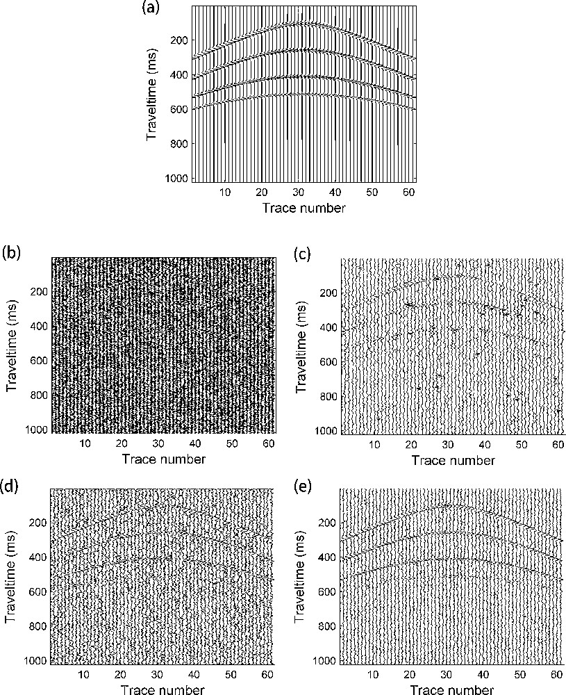
Results after filtering synthetic seismic data with low SNR: (a) four Ricker wavelets of dominant frequencies 25 Hz, 30 Hz, 35 Hz and 40 Hz were used to simulate synthetic waveforms as natural events; (b) noisy seismic data (SNR = –15 dB) contaminated with white Gaussian noise; (c) result after using the wavelet-transform filtering method; (d) result after using conventional TFPF; (e) result after using modified TFPF.

6 Denoising with field seismic data

To verify the versatility of the proposed method, we applied it to field seismic data. We have considered a common shot point seismic gather for testing, as shown in Fig. 7a. The spatial gap between geophones is 30 m and the traces are sampled with a frequency of 1000 Hz. Again, we have contrasted the results obtained through modified TFPF with those obtained with conventional TFPF and the wavelet-transform filtering method. As can be seen, when comparing the results to each other, the latter method and the conventional TFPF method do not reduce the random noise (Fig. 7b, c, respectively) with the same effectiveness that the modified TFPF (Fig. 7d), such as is highlighted within the rectangles. To visually assessing the quality of the results, we show an enlarged view between traces 6–69 and double time 701–1724 ms in Fig. 8a. The reflection events processed through modified TFPF (Fig. 8d) are more clearly recovered, as well as the continuity of the energy arrivals (see in the interior of the ellipses) than with the other two methods (Fig. 8b, c). According to these experimental results, the proposed seismic denoising method has a greater advantage for eliminating random noise and preserving the reflection events more efficiently if we compare it with the other two methods.

Fig. 7
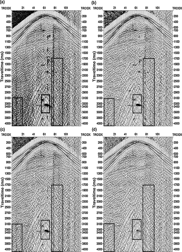
Results obtained with field seismic data after using conventional and modified time-frequency peak filtering: (a) field data (common shot point seismic data); (b) after applying the wavelet-transform filtering method; (c) by using conventional TFPF; (d) by using modified TFPF. Rectangles delimit those areas where we can better observe the progressive efficiency of the filtering.

Fig. 8
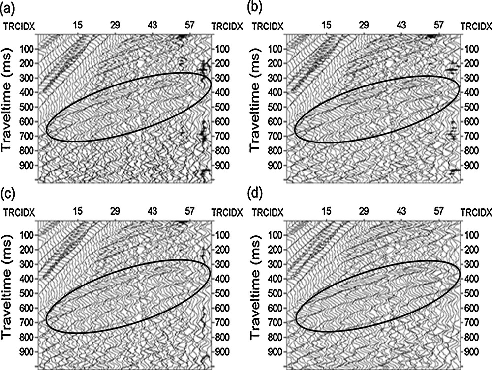
An enlarged view allowing seeing the quality of the filtering between the traces 6 to 69 and double travel times 701 to 1724 ms: (a) unfiltered seismic parts; (b) filtered seismic sections using wavelet transform filter; (c) filtered seismic sections using conventional TFPF; (d) filtered seismic sections using modified TFPF.

7 Conclusions

We have developed an effective time-frequency distribution to improve the denoising performance of TFPF on noisy seismic signals. The distribution follows a four-step working scheme, namely: (a) calculation of the pseudo Wigner–Ville distribution PWVD; (b) smoothing in time and frequency by means of a double window to obtain SPWVD; (c) use of a step function to remove divergent time-frequency points and to obtain $SP \hat{W} VD$ ; (d) computation of the joint time-frequency distribution JTFD from PWVD weighted by $SP \hat{W} VD$ . The usefulness of the modified time-frequency peak filtering based on JTFD has been checked with synthetic and real seismic data, and also contrasted with conventional TFPF and the wavelet-transform filtering method. The results demonstrate that modified TFPF gives smaller MSEs and higher quality signals recovered from noisy signals. The proposed method has a clear effect on suppressing random noise and can recover seismic events with a greater effectiveness. Therefore, the method presented here has wide applicability, especially in the case of noisy seismic signals with low signal-to-noise ratio.

Acknowledgments

We would like to thank the two reviewers for their constructive comments that helped us to greatly improve the early version of the manuscript. The National Natural Science Foundation of China (grants Nos. 41130421 and 41274118), the Science and Technology Development Program of Jilin Province of China (grant No. 20110362) and the Development and Reform Commission of Jilin Province (grants No. 2011006-2, JF2012C013-2) financially supported this research.

Bibliographie

[Auger and Flandrin, 1995] F. Auger; P. Flandrin Improving the readability of time-frequency and time-scale representations by the reassignment method, IEEE Trans. Signal Process., Volume 43 (1995), pp. 1068-1089

[Barbarossa, 1997] S. Barbarossa Parameter estimation of spread spectrum frequency hopping signals using time-frequency distributions, First IEEE Signal Processing Workshop on Signal Processing Advances in Wireless Communications, (1997), pp. 213-216

[Barkat and Boashash, 1999] B. Barkat; B. Boashash Design of higher order polynomial Wigner–Ville distributions, IEEE Trans. Signal Process., Volume 47 (1999), pp. 2608-2611

[Boashash and Mesbah, 2004] B. Boashash; M. Mesbah Signal enhancement by time-frequency peak filtering, IEEE Trans. Signal Process., Volume 52 (2004), pp. 929-937

[Cao and Chen, 2005] S.Y. Cao; X.P. Chen The second generation wavelet transform and its application in denoising of seismic data, Appl. Geophys., Volume 2 (2005), pp. 70-74

[Duncan and Beresford, 1995] G. Duncan; G. Beresford Median filter behavior with seismic data, Geophys. Prospect., Volume 43 (1995), pp. 329-345

[Ghias et al., 2007] R.A. Ghias; M.B. Shamsollahi; M. Mobed Estimation of modal parameters using bilinear joint time-frequency distributions, Mech. Syst. Signal Pr., Volume 21 (2007), pp. 2125-2136

[Lin et al., 2007] H.B. Lin; Y. Li; B.J. Yang Recovery of seismic events by time-frequency peak filtering, IEEE International Conference on Image Processing, Volume 5 (2007), pp. 441-444

[Lu et al., 2006] W.K. Lu; W.P. Zhang; D.Q. Liu Local linear coherent noise attenuation based on local polynomial approximation, Geophysics, Volume 71 (2006), pp. 105-110

[Lu, 2006] W.K. Lu Adaptive noise attenuation of seismic images based on singular value decomposition and texture direction, J. Geophys. Eng., Volume 3 (2006) no. 1, pp. 28-34

[Wang, 1999] Y. Wang Random noise attenuation using forward-backward linear prediction, J. Seism. Explor., Volume 8 (1999), pp. 133-142

[Wang, 2002] Y. Wang Seismic trace interpolation in the f–x-y domain, Geophysics, Volume 67 (2002), pp. 1232-1239

[Wu et al., 2011] N. Wu; Y. Li; B.J. Yang Noise attenuation for 2-D seismic data by radial-trace time-frequency peak filtering, IEEE Geosci. Remote Sensing Lett., Volume 8 (2011), pp. 874-878

[Zahir and Hussain, 2000] M. Zahir; B. Hussain Adaptive Instantaneous frequency estimation of multicomponent FM signal using quadratic time-frequency distributions, IEEE Trans. Signal Process., Volume 50 (2000), pp. 657-660

[Zhang and Klemperer, 2005] Z.J. Zhang; S.L. Klemperer West–east variation in crustal thickness in northern Lhasa block central Tibet, from deep seismic sounding data, J. Geophys. Res., Volume 110 (2005), p. B0943

Commentaires - Politique

Ces articles pourraient vous intéresser

Seismic random noise attenuation and signal-preserving by multiple directional time-frequency peak filtering

Chao Zhang; Yue Li; Hong-bo Lin; ...

C. R. Géos (2015)

Trace-transform-based time-frequency filtering for seismic signal enhancement in Northeast China

Ning Wu; Yue Li; Yanan Tian; ...

C. R. Géos (2016)

Seismic random noise elimination according to the adaptive fractal conservation law

Fanlei Meng; Yue Li; Qian Zeng

C. R. Géos (2016)