Jump conditions and dynamic surface tension at permeable interfaces such as the inner core boundary

Frédéric Chambat; Sylvie Benzoni-Gavage; Yanick Ricard

doi:10.1016/j.crte.2014.04.006

Internal geophysics (Physics of Earth's interior)

Jump conditions and dynamic surface tension at permeable interfaces such as the inner core boundary

Frédéric Chambat ¹ ; Sylvie Benzoni-Gavage ² ; Yanick Ricard ³

¹ Laboratoire de géologie de Lyon, CNRS UMR 5276, École normale supérieure de Lyon, 46, allée d’Italie, 69364 Lyon cedex 07, France
² Institut Camille-Jordan, CNRS UMR 5208, Université de Lyon, Université Claude-Bernard Lyon-1, bâtiment Braconnier, 43, boulevard du 11-Novembre-1918, 69622 Villeurbanne cedex, France
³ Laboratoire de géologie de Lyon, CNRS UMR 5276, Université de Lyon, Université Claude-Bernard Lyon-1, bâtiment Géode, 2, rue Raphaël-Dubois, 69622 Villeurbanne cedex, France

Comptes Rendus. Géoscience, Volume 346 (2014) no. 5-6, pp. 110-118.

Résumé

We consider a fluid crossing a zone of rapid density change, so thin that it can be considered as a density jump interface. In this case, the normal velocity undergoes a jump. For a Newtonian viscous fluid with low Reynolds number (creeping flow) that keeps its rheological properties within the interface, we show that this implies that the traction cannot be continuous across the density jump because the tangential stress is singular. The appropriate jump conditions are established by using the calculus of distributions, taking into account the curvature of the interface as well as the density and viscosity changes. Independently of any intrinsic surface tension, a dynamic surface tension appears and turns out to be proportional to the mass transfer across the interface and to a coefficient related to the variations of density and viscosity within the interface. Explicit solutions are exhibited to illustrate the importance of these new jump conditions. The example of the Earth's inner core crystallisation is questioned.

Métadonnées

Reçu le : 2014-03-25
Accepté le : 2014-04-12
Publié le : 2014-05-01

DOI : 10.1016/j.crte.2014.04.006

Mots clés : Fluid mechanics, Phase change, Jump conditions

Affiliations des auteurs :

Frédéric Chambat ¹ ; Sylvie Benzoni-Gavage ² ; Yanick Ricard ³

@article{CRGEOS_2014__346_5-6_110_0,
     author = {Fr\'ed\'eric Chambat and Sylvie Benzoni-Gavage and Yanick Ricard},
     title = {Jump conditions and dynamic surface tension at permeable interfaces such as the inner core boundary},
     journal = {Comptes Rendus. G\'eoscience},
     pages = {110--118},
     publisher = {Elsevier},
     volume = {346},
     number = {5-6},
     year = {2014},
     doi = {10.1016/j.crte.2014.04.006},
     language = {en},
}

TY  - JOUR
AU  - Frédéric Chambat
AU  - Sylvie Benzoni-Gavage
AU  - Yanick Ricard
TI  - Jump conditions and dynamic surface tension at permeable interfaces such as the inner core boundary
JO  - Comptes Rendus. Géoscience
PY  - 2014
SP  - 110
EP  - 118
VL  - 346
IS  - 5-6
PB  - Elsevier
DO  - 10.1016/j.crte.2014.04.006
LA  - en
ID  - CRGEOS_2014__346_5-6_110_0
ER  -

%0 Journal Article
%A Frédéric Chambat
%A Sylvie Benzoni-Gavage
%A Yanick Ricard
%T Jump conditions and dynamic surface tension at permeable interfaces such as the inner core boundary
%J Comptes Rendus. Géoscience
%D 2014
%P 110-118
%V 346
%N 5-6
%I Elsevier
%R 10.1016/j.crte.2014.04.006
%G en
%F CRGEOS_2014__346_5-6_110_0

Frédéric Chambat; Sylvie Benzoni-Gavage; Yanick Ricard. Jump conditions and dynamic surface tension at permeable interfaces such as the inner core boundary. Comptes Rendus. Géoscience, Volume 346 (2014) no. 5-6, pp. 110-118. doi : 10.1016/j.crte.2014.04.006. https://comptes-rendus.academie-sciences.fr/geoscience/articles/10.1016/j.crte.2014.04.006/

Version originale du texte intégral

1 Introduction

Jump conditions to be applied across an interface within a viscous fluid have been explored for several decades (Anderson et al., 1998, 2007; Aris, 1962; Delhaye, 1974; Dziubek, 2011; Ishii and Hibiki, 2011; Joseph and Renardy, 1993; Slattery et al., 2007). A general form of the traction jump (the traction is σn where σ is the stress tensor and n a unit vector normal to the interface) involves a flux of momentum across the interface, a possibly anisotropic surface tension and terms including an interface mass density. In pratice, the interface is often supposed to have no mass and the traction is known to undergo a jump especially in two cases: in a shock wave, where the flux of momentum across the interface equals the jump of pressure; and in the presence of surface tension defined as a capillary action due to intermolecular forces at the interface between two immiscible fluids.

Here, we put aside the shock wave and the intrinsic surface tension contributions. In this case, the traction vector is usually supposed to be continuous, for example across phase changes (Hutter and Johnk, 2004). On the contrary, in this paper we show: first, that when a viscous fluid with low Reynolds number crosses an interface with a density jump the traction undergoes a jump; second that this jump takes the mathematical form of an isotropic surface tension that we obtain as a function of the fluid parameters.

The question of a discontinuous traction was first addressed in the context of solid Earth geophysics (Corrieu et al., 1995). Indeed, on a time scale of millions of years, Earth's mantle behaves as a viscous quasi-static fluid that enables convection due to cooling at the external surface and to internal heat sources (decay of radioactive elements). Transported with this movement, Earth's minerals undergo various phase changes due to the large increases in pressure and temperature with depth (and modestly, their variations with latitude and longitude). In Earth, the major phase transitions are located at 410 and 670 km depths and are associated with ∼ 10% density jumps. The physics of these phase changes are complicated as they occur across regions of partial change including a mixture of both phases but each is sharp enough to be modelled as a discontinuity in fluid dynamic simulations of mantle convection. Until now, in simulations the traction jump was supposed to be null at these interfaces (Alboussière et al., 2010; Monnereau et al., 2010; Roberts et al., 2007; Schubert et al., 2001; Sotin and Parmentier, 1989). Concerning the deepest discontinuity in the Earth, a translational convection of the inner solid core within the fluid metallic core has been predicted (Alboussière et al., 2010; Monnereau et al., 2010). This mode relies on a mass flux at the interface, the inner core permanently cristallising on one side and melting on the other. The plausibility of this motion depends however on the traction conditions at the surface of the inner core.

In the context of Earth's convection, Corrieu et al. (1995) noticed however that a stress continuity across a phase jump led to inconsistencies: applying a null traction jump did not yield the same results as solving numerically the Stokes equations within the phase change discontinuity. The authors derived the corresponding jump condition in the special case of a spherical interface, with linear variations of density and viscosity with depth within the transition zone. Ricard (2007) addressed this question again, confirmed that the traction is not continuous and expressed its jump in the case of a plane interface and a uniform viscosity.

The purpose of the present paper is to examine this question in a more general framework, for interfaces of arbitrary curvature, density and Newtonian viscosity variations. The model is justified in the geophysical context but can be considered as rather specific in general fluid mechanics: it is fully dominated by viscous stresses (small Reynolds number) and the density variations of the background are fixed and represented by a discontinuity. Notice however that the problem appearing in the case of a creeping flow should also be present in the case of finite Reynolds numbers. We show that in the case of a density jump there must be an equivalent surface tension to ensure global conservation of momentum, and that this tension is given in terms of the mass transfer flux and of the density and viscosity changes by Eqs. (25)–(26). Upon applications, this effect may influence the inner core crystallisation.

In the next sections, we point out how the traction jump appears in two simple cases. Then, the following section is devoted to the expression and proof of the traction jump in a general case: we look for weak solutions of the Stokes equations that are smooth on either side of an arbitrarily curved interface, and thus obtain the announced jump conditions.

2 Existence and necessity of a traction jump

Searching the interface condition is related to the following question: if a velocity and stress field is a solution of the Stokes equations for a continuous but rapidly varying density, can this solution be approximated by the one for a sharp interface and what are the corresponding jump conditions? We illustrate the problem with two simple situations, first with a flat interface, then with a curved interface.

2.1 Existence of a traction jump across a flat interface

We consider a 2D compressible, viscous, quasi-static liquid, in steady-state regime, through the rectangular volume −h < z < h and −π/k < x < π/k. A mass flux ψ₀ cos kx is injected at z = −h and extracted at z = h. To mimic a phase transition that would occur near z = 0, we assume that the density ρ(z) changes continuously from ρ⁻ to ρ⁺ between z = −ɛ and z = ɛ and we solve for the flow υ (x, y) in the whole domain. Considering that a phase change occurs across a very thin z-interval, this situation is expected to close to the situation where the density changes discontinuously at z = 0 and where jump conditions are implemented across the discontinuity. We show however that the continuous approach when ɛ→0 does not converge to the discontinuous approach where the traction is supposed continuous.

The Stokes equations governing a viscous linear quasi-static fluid are:

\nabla \cdot (ρ υ) = 0,

(1)

\nabla \cdot σ = 0,

(2)

σ = - p I + η (\nabla υ + {(\nabla υ)}^{T}) + λ (\nabla \cdot υ) I,

(3)

where ρ is the fluid density, υ its velocity, σ the stress tensor, p the pressure, η and λ the shear and bulk viscosities, and I the identity tensor.

According to the first relation, ρυ can be sought of the form $ρ υ_{x} = - \partial_{z} Ψ, ρ υ_{z} = + \partial_{x} Ψ$ ; with the curl of relation (2), and assuming constant η, it implies that

Δ (\nabla \cdot (\frac{1}{ρ} \nabla Ψ)) = 0 .

(4)

At z = ± h we impose the sinusoidal vertical flux:

\partial_{z} Ψ (x, z = \pm h) = 0,

(5)

\partial_{x} Ψ (x, z = \pm h) = Ψ_{0} \cos k x .

(6)

Solutions of the form $Ψ = \hat{Ψ}$ (z) sin (kx) are easy to find numerically as $\hat{Ψ}$ is the solution of a fourth order linear and homogeneous differential system in z. Using a Runge–Kutta method, four elementary solutions are computed in each domain where the parameters are continuous (i.e., in the whole domain when the density evolves continuously, in the two subdomains z < 0 and z > 0 when the density is discontinuous), then the general solution is found by linearly combining these solutions, with coefficients determined by solving the linear system corresponding to the limit and jump conditions. In that way we compute three types of solutions:

• a solution with a smooth but rapidly varying density ρ = ρ_ɛ (Fig. 1, solid black line). We choose ρ_ɛ(z) = ρ^– + (ρ⁺ – ρ^–) (tanh (z/ɛ)+ 1)/2, which, for small ɛ is close to the function $ρ_{0} = ρ^{-} 1^{-} + ρ^{+} 1^{+} where 1^{\pm}$ denotes the characteristic functions of the half-spaces $z ≷ 0$ .
• a solution with a discontinuous density ρ = ρ₀ (Fig. 1, dashed red line), a continuous mass flux (ρυ_z) and traction at z = 0. These are the usual conditions for a flow crossing a phase change, neglecting surface tension.
• a solution with a discontinuous density ρ = ρ₀, a continuous mass flux and a discontinuous traction at z = 0 as proposed later in this paper.

Fig. 1
Left: density models used: continuous density ρ_ɛ (black/full line) and discontinuous density ρ₀ (red/dashed line) as a function of z.

Although the vertical velocities are visually similar (Fig. 2, top row), the results for the horizontal velocity (bottom row) are surprisingly different. This suggests that the limit of a diffuse layer (solution [a], left panel) is not a sharp interface with a continuous traction (solution [b], middle panel) but a sharp interface with an equivalent dynamic surface tension (solution [c], right panel).

Fig. 2
(Color online.) Velocities for the solutions as functions of x and z: top row υ_z, bottom row υ_x. Left panels: numerical solution for a diffuse interface (ρ = ρ_ɛ). Middle: numerical solution for a sharp interface (ρ = ρ₀) by using the usual jump conditions (continuous traction). Right: numerical solution for a sharp interface (ρ = ρ₀) by using our jump conditions (discontinuous traction). In this example, we have taken ρ⁻ = 1, ρ⁺ = 2, h = 1, k = π/5, η = 1, ɛ = 0.03.

To understand where the problem lies, we plot on Fig. 3, the profiles of the shear stress σ_xz(x = π/(2k), z) (left) and vertical stress σ_zz(x = 0, z) (right), at x = 0. It is obvious that the shear stress profile computed for the rapid and continuous density change (solution [a], solid line, left panel) looks rather discontinuous and can hardly converge toward the smooth solution computed with the usual jump conditions on interfaces (solution [b], blue dotted-dashed line, left panel). The profiles for the vertical stress are continuous but remain clearly different (right panel). The solution computed with a continuous mass flux and a discontinuous traction at z = 0 as proposed later in this paper (solution [c] red dashed lines) provides clearly a much better fit to the stresses computed with a continuous density change (solution [a], solid lines).

Fig. 3
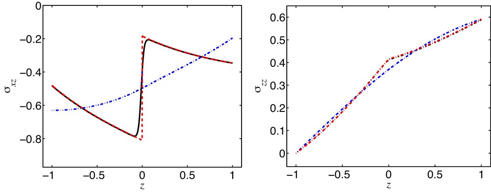
Left: normal stress σ_xz at kx = π/2 as a function of z. Right: normal stress σ_zz at x = 0 as a function of z. In each panel, the three curves are for a continuous density ρ_ɛ (black line), a discontinuous density and continuous traction (blue), a discontinuous density and discontinuous traction (red). Same parameters as on Fig. 2. (For interpretation of the references to color in this figure, the reader is referred to the web version of this article).

This simple example, which can be interpreted as a naive view of mantle convection with a hot mantle crossing a phase transition in between two subducting slabs, illustrates therefore a situation where the usual jump conditions on interface do not hold and where the shear stress is discontinuous on an interface without intrinsic surface tension.

2.2 The necessity of a traction jump

Let us now explain in a heuristic way why the traction must have a jump across a density jump with a mass transfer. As in the example before, the interface is considered as a layer in between z = −ɛ and z = +ɛ inside which Eqs. (1)–(3) hold and all the fluid parameters vary significantly faster in the z-direction than in the x-direction.

The thought experiment consisting in considering ɛ→0 is called in most textbooks the “pillbox” argument. Mathematically speaking, we start from a family of rapidly varying but still smooth densities ρ_ɛ, and viscosities λ_ɛ and η_ɛ, converging pointwise when ɛ goes to zero to some functions ρ, λ and η that are possibly discontinuous at z = 0 – which means that the limiting sharp interface is located at z = 0. Then we assume that with those “mollified” coefficients ρ_ɛ, λ_ɛ, η_ɛ, the 2D Stokes equations have solutions υ_ɛ converging pointwise to υ, and we look for jump conditions on υ. The general idea is that ρ_ɛ, λ_ɛ, η_ɛ, υ_ɛ, and their x-derivatives remain bounded in the limit ɛ→0, whereas the z-derivative of any of those quantities that is discontinuous in the limit blows up as 1/ɛ. For simplicity, we omit the subscript ɛ in what follows.

In 2D, the Stokes Eqs. (1)–(3) read:

\partial_{z} (ρ υ_{z}) + \partial_{x} (ρ υ_{x}) = 0

(7)

\partial_{z} σ_{z z} + \partial_{x} σ_{x z} = 0

(8)

\partial_{z} σ_{x z} + \partial_{x} σ_{x x} = 0

(9)

σ_{x z} = η (\partial_{x} υ_{z} + \partial_{z} υ_{x})

(10)

σ_{z z} = - p + 2 η \partial_{z} υ_{z} + λ (\partial_{x} υ_{x} + \partial_{z} υ_{z})

(11)

σ_{x x} = - p + 2 η \partial_{x} υ_{x} + λ (\partial_{x} υ_{x} + \partial_{z} υ_{z}) .

(12)

Eq. (7) readily shows that ρυ_z must remain continuous in the limit ɛ→0 (otherwise, ∂_x(ρυ_x) = −∂_z(ρυ_z) would blow up). If we denote by $〚〛$ the jump of a quantity across the interface, this usual jump condition reads $〚ρ υ_{z}〛 = 0$ . By the same argument, the usual jump conditions are obtained by considering that equations (8) and (9) imply $〚σ_{z z}〛 = 0 and 〚σ_{x x}〛 = 0$ , respectively, provided that ∂_xσ_xz and ∂_xσ_xx be bounded. However, the latter assumption is unlikely to hold true if the mass transfer flux ρυ_z is nonzero. Indeed, subtracting (11) to (12) we obtain

σ_{x x} = σ_{z z} + 2 η (\partial_{x} υ_{x} - \partial_{z} υ_{z}) .

(13)

The important point is that the vertical velocity becomes discontinuous when the thickness ɛ→0 and that ∂_zυ_z blows up. As suggested by Fig. 3, σ_zz remains bounded (and continuous) and as ∂_xυ_x is also bounded, σ_xx must blow up too. In (9), the two terms blow up as 1/ɛ and one cannot infer that $〚σ_{x z}〛 = 0$ anymore.

To derive the appropriate jump, we use (9) and (13) and find that

\partial_{z} σ_{x z} = - \partial_{x} σ_{x x} = - \partial_{x} σ_{z z} - 2 \partial_{x} (η (\partial_{x} υ_{x} - \partial_{z} υ_{z}))

(14)

In the right-hand side, only the term in ∂_zυ_z is singular in the limit ɛ→0, thus by integration across the layer (Anderson et al., 1998) on a height 2δ such that $ε ≪ δ ≪ 1$ we get $〚σ_{x z}〛 = 2 \lim_{ε \to 0} \partial_{x} \int_{- δ}^{δ} η \partial_{z} υ_{z} d z .$ With the mass conservation (7) it implies $〚σ_{x z}〛 = - 2 \lim_{ε \to 0} \partial_{x} \int_{- δ}^{δ} η (\partial_{z} ρ) υ_{z} / ρ d z$ or since ρυ_z is continuous:

〚σ_{x z}〛 = - 2 \partial_{x} (ρ v_{z} \lim_{ε \to 0} \int_{- δ}^{δ} η (\partial_{z} ρ) / ρ^{2} d z) .

(15)

This can be written

〚σ_{x z}〛 = 2 \partial_{x} (〚ν〛 ρ υ_{z})

(16)

where

〚ν〛 = \lim_{ε \to 0} \int_{- δ}^{δ} η \partial_{z} (1 / ρ) d z

(17)

is the jump of the function

\int η \partial_{z} (1 / ρ) d z .

Notice that

〚ν〛

involves variation of parameters within the interface although it can be written as a jump.

The jump conditions for a plane interface are therefore:

\begin{array}{l} 〚ρ υ_{z}〛 = 0 〚σ_{z z}〛 = 0 \\ 〚υ_{x}〛 = 0 〚σ_{x z}〛 = 2 \partial_{x} (〚v〛 ρ υ_{Z}) . \end{array}

(18)

With a constant viscosity within the interface we get $〚ν〛 = η 〚1 / ρ〛$ , and since the first relation implies $〚1 / ρ〛 ρ υ_{z} = 〚υ_{z}〛$ the fourth equation also reads $〚σ_{x z}〛 = 2 \partial_{x} (η 〚υ_{z}〛) .$ The correct jump condition yields $〚\partial_{z} υ_{x}〛 - \partial_{x} 〚υ_{z}〛 = 0$ while the traditional condition $〚σ_{x z}〛 = 0$ implies $〚\partial_{z} υ_{x}〛 + \partial_{x} 〚υ_{z}〛 = 0!$

According to (13), σ_xx becomes infinite in the limit ɛ→0. Using the same kind of integration as for the proof of (16), its integral across the infinitely thin interface is

s ≔ \lim_{ε \to 0} \int_{- δ}^{δ} σ_{x x} d z = - 2 〚ν〛 ρ υ_{z} .

(19)

s is therefore a force per unit length, a tension embedded in the interface, similar to the surface tension on the interface of immiscible fluids. As for the Marangoni effect (Pearson, 1958), the fourth relation of (18) yields a traction along the interface that is proportional to the surface tension gradient:

〚σ_{x z}〛 = - \partial_{x} s

. However, s is not an intrinsic property of the interface, but a dynamic property of the flow.

When the flow crosses a density interface, the pillbox argument cannot be used without including lateral terms because, in the same way as in the presence of intrinsic surface tension (Anderson et al., 1998), the lateral stress diverges when the pillbox shrinks and thus the lateral integrals do not vanish in the zero-height limit.

To summarize, we expect that for a viscous fluid (η ≠ 0) with mass transfer at the interface (ρυ_z ≠ 0), both p and σ_xx become singular – like across an interface endowed with intrinsic surface tension – while ρυ_z and υ_x are continuous, and the other stress components σ_xz and σ_zz may have jumps (for a flat interface, the latter is not affected by surface tension).

As we have seen that a rapid density change implies the existence of an equivalent surface tension, we should now verify that the normal stress discontinuity occurring across a curved interface (the Young–Laplace condition) is also valid in the case of a rapid density change.

2.3 Existence of a traction jump across a curved interface

We consider a simple flow diverging from a point source with radial velocity $υ = υ (r) \hat{r}$ , with a density ρ (r) varying rapidly from ρ⁻ to ρ⁺ across a shell located between the radii R − δ and R + δ. In this spherically symmetric situation the solution of Stokes equations is even more surprising since we can prove analytically (and very simply) the existence of a dynamic surface tension. Indeed, with η = η (r) and λ = λ (r), the only nonzero stress is $σ_{r r} = - p + 2 η \partial_{r} υ + λ \partial_{r} (r^{2} υ) / r^{2}$ and $σ_{θ θ} = σ_{ϕ ϕ} = - p + 2 η υ / r + λ \partial_{r} (r^{2} υ) / r^{2}$ and the equilibrium equation yields

\partial_{r} σ_{r r} + 4 η \partial_{r} (\frac{υ}{r}) = 0 .

(20)

The mass conservation equation implies

ρ υ = \frac{C}{r^{2}}

(21)

where C is a constant. By combining these two equations we get

\partial_{r} σ_{r r} + 4 η \frac{ρ υ}{r} \partial_{r} (1 / ρ) - 12 η \frac{υ}{r} = 0 .

(22)

The last term is bounded, ρυ/r is continuous, therefore by integration across the discontinuity

〚σ_{r r}〛 = - 4 \frac{ρ υ}{R} \lim_{ε \to 0} \int_{R - δ}^{R + δ} η \partial_{r} (1 / ρ) d r = \frac{2 s}{R} .

(23)

As in the Young–Laplace law, the jump of normal stress is not zero but proportional to the total curvature 2/R and to the surface tension which is here $- 2 〚ν〛 ρ υ$ , in agreement with what we found across a flat interface. This effect may be large, as the jump $(2 s / R \sim 4 η 〚1 / ρ〛 ρ υ / R)$ and the viscous stress $(\sim η υ / R)$ have similar magnitudes. In this example, that can be seen as a naive view of the crystallising inner core, the usual jump conditions on interface also do not hold, and the normal stress is discontinuous on an interface without intrinsic surface tension.

3 Jump conditions

3.1 Statement of jump conditions

We now give the general jump conditions for a general 3D fluid having a curved interface. We consider a fluid verifying eqs. (1)–(3) everywhere, and undergoing a density jump when crossing a static surface $Σ = \{x |q^{3} = 0\}$ , with q³ a local coordinate normal to the surface. We suppose that this mathematical surface corresponds physically to a very small layer in which the Stokes equations remain valid. We neglect intrinsic surface tension on the interface Σ. The jump of any piecewise-smooth quantity f across the interface at $x \in Σ$ is defined as $〚f〛 = f^{+} - f^{-} ≔ \lim_{ε \to 0^{+}} f (x + ε n) - \lim_{ε \to 0^{+}} f (x - ε n)$ where n denotes the unit normal to the interface at point x and pointing towards positive q³. In addition, we use the subscript _T for the tangential part $υ_{T} = υ - (υ \cdot n) n$ of a vector field υ on Σ. Accordingly, $\nabla_{T}$ and $\nabla_{T} \cdot$ stand for the tangential gradient and tangential divergence on Σ (Slattery et al., 2007). Then in particular, $κ = \nabla_{T} \cdot n$ is the sum of principal curvatures of Σ. The main result of the paper is that, apart from the usual jump conditions

〚ρ υ \cdot n〛 = 0, 〚υ_{T}〛 = 0,

(24)

we have

〚σ n〛 = s κ n - \nabla_{T} s,

(25)

i.e. the traction jump has exactly the same form as in the case of (intrinsic) isotropic surface tension (Joseph and Renardy, 1993), but here s is a dynamic surface tension, given by

s ≔ - 2 〚ν〛 ρ υ \cdot n

(26)

where

〚ν〛

is the jump of the function

\int η \partial_{q^{3}} (1 / ρ) d q^{3}

. This quantity is homogeneous with a kinematic viscosity and depends on variations of both ρ and η “inside” the interface and

ρ υ \cdot n

is the mass flux across the interface. We have introduced the minus sign in eq. (26) in agreement with the usual convention sign of the surface tension in (25). The important point is that this dynamic surface tension is not intrinsic but a function of the fluid parameters and of the mass flux. We recover what was found in particular cases (Corrieu et al., 1995; Ricard, 2007); indeed with the useful relation:

〚\frac{1}{ρ}〛 ρ υ \cdot n = 〚υ \cdot n〛

(27)

and in the case of uniform viscosity for example (Ricard, 2007), we get

〚ν〛 ρ υ \cdot n = η 〚υ \cdot n〛

The usual jump conditions on a phase change interface consist of eq. (24) together with $〚σ n〛 = 0$ (Hutter and Johnk, 2004). The latter is recovered from (25) when the dynamic surface tension s vanishes identically, which is the case for an impermeable interface (thus with null mass flux) or if the density is uniform. The traction continuity is recovered too when the interface is flat and the dynamic surface tension s is uniform.

For the sake of simplicity, inertia, surface forces, surface mass density and any a priori intrinsic surface tension have been neglected. These effects are taken into account by well-known jump conditions (Slattery et al., 2007). The main result of the paper is that without any intrinsic surface tension there still exists another surface tension, but of a dynamic origin, which is explicitely given as a function of the fluid parameters by (26).

3.2 Proof of jump conditions

Finding the jump conditions amounts to investigate the (very) weak solutions to the Stokes equations which are expected from a passage to the limit ɛ→0 as in Section 2.2. For that purpose we look for jump conditions on solutions of (1)–(3) in the sense of distributions, with discontinuous coefficients ρ, λ, η across a smooth surface Σ.

We denote by ψ(x) the signed distance of the point x to the surface. The equation of the surface is ψ(x) = 0, and in a vicinity of the surface ψ satisfies the eikonal equation $∥\nabla ψ (x)∥ = 1$ and defines the unit normal $n ≔ \nabla ψ (x)$ . We denote by x₁, x₂, x₃ = x, y, z the Cartesian coordinates of x, and we adopt the usual convention of summation over repeated indices. For convenience we rewrite the eq. (2) with indices:

\partial_{j} (- p + λ \partial_{i} υ_{i}) + \partial_{i} (η (\partial_{i} υ_{j} + \partial_{j} υ_{i})) = 0, j \in \{1,2,3\},

(28)

or, in short, as L(p, υ) = 0 where L is the Stokes operator

(p, υ) \mapsto L (p, υ) ≔ \nabla (- p + λ \nabla \cdot υ) + \nabla \cdot (η (\nabla υ + {(\nabla υ)}^{T})) .

(29)

A usual method to get jump conditions is to find the discontinuous solutions of the corresponding operator (Bedeaux et al., 1976). Thus, we assume that the velocity field is of the form

υ = υ^{-} 1^{-} + υ^{+} 1^{+},

(30)

and that the pressure term is of the form

p = p^{-} 1^{-} + p^{+} 1^{+} + P δ,

(31)

where υ^±, p^± are smooth functions of x on the half-spaces

\{x = (x_{1}, x_{2}, x_{3}); ψ (x) \geq 0\}, \{x = (x_{1}, x_{2}, x_{3}); ψ (x) \leq 0\},

(32)

while

1^{+} ≔ 1_{ψ} \geq 0

and

1^{-} ≔ 1_{ψ} \geq 0

denote the characteristic functions of these half-spaces,

δ = δ (ψ)

stands for the Dirac mass on their separating surface Σ, and

P

is a smooth function of x on Σ and its vicinity.

In what follows, we repeatedly use the following calculus formulas (Bedeaux et al., 1976; Gel’fand and Shilov, 1968, chap. 3.1):

\partial_{j} 1 \pm = \pm (\partial_{j} ψ) δ, \partial_{j} δ = (\partial_{j} ψ) δ^{'},

(33)

where the latter follows from the definition of the surface distribution

δ^{'} = δ^{'} (ψ)

Then, the derivatives of p and υ in the sense of distributions are

\partial_{j} p = (\partial_{j} p^{-}) 1^{-} + (\partial_{j} p^{+}) 1^{+} + 〚p〛 (\partial_{j} ψ) δ + P (\partial_{j} ψ) δ^{'},

(34)

\partial_{j} υ = (\partial_{j} υ^{-}) 1^{-} + (\partial_{j} υ^{+}) 1^{+} + 〚υ〛 (\partial_{j} ψ) δ .

(35)

For convenience, we extend υ^± in a smooth manner to the other sides of Σ, so that the jump $〚υ〛$ is extended to a smooth function in the vicinity of Σ, merely defined as $〚υ〛 = υ^{+} - υ^{-}$ . In the same way we extend p^± and $P$ .

For the sake of clarity, we start with λ and η continuous across the interface and postpone our more elaborate calculation intended for general interfaces to the next section.

3.2.1 Continuous rheology

Let us first derive jump conditions in the special case when all products in (28) are well defined, that is, assuming that both viscosities λ and η are regular, and more especially constant across Σ.

Differentiating once more in the sense of distributions and using $\partial_{j} ψ = n_{j}$ and (33) we find that the Stokes equations L(p, υ) = 0 are equivalent to L(p^±, υ^±) = 0 and m(p, υ) = 0, where m(p, υ) is the vector-valued distribution supported by Σ whose components are

m_{j} (p, υ) = \begin{array}{l} - 〚p〛 n_{j} δ & - (\partial_{j} P) δ & - P n_{j} δ^{'} \\ + 〚λ \partial_{i} υ_{i}〛 n_{j} δ & + \partial_{j} (〚λ υ_{i}〛 n_{i}) δ & + 〚λ υ_{i}〛 n_{i} n_{j} δ^{'} \\ + 〚η \partial_{i} υ_{j}〛 n_{i} δ & + \partial_{i} (〚η υ_{j}〛 n_{i}) δ & + 〚η υ_{j}〛 n_{i} n_{i} δ^{'} \\ + 〚η \partial_{j} υ_{i}〛 n_{i} δ & + \partial_{i} (〚η υ_{i}〛 n_{j}) δ & + 〚η υ_{i}〛 n_{j} n_{i} δ^{'}, \end{array}

(36)

where we intentionally leave λ and η inside the jumps to insist on the fact that it must be evaluated at

ψ = 0

Now we use that for any smooth functions a(x) and b(x), the equality aδ + bδ′ =0 is equivalent to b = 0 and $a = n_{j} \partial_{j} b$ on the interface Σ (here, $δ^{'} = n_{j} \partial_{j} δ$ is a normal derivative, eq. (33), so that $a δ + b δ^{'}$ applied to any test function f, is the value of $a f - \partial_{j} (n_{j} b f) = (a - b \partial_{j} n_{j} - n_{j} \partial_{j} b) f - b n_{j} \partial_{j} f$ taken on the interface). In this paper, b will represent functions defined on the interface only, thus their extension outside Σ does not play any role and we can assume, for convenience and without loss of generality, that their normal derivative is zero. Thus, $a δ + b δ^{'} = 0$ will be equivalent to b = 0 and a = 0 on Σ (Bedeaux et al., 1976, appendix A).

Thus, collecting the δ′ terms of (36) and equating their sum to zero, we infer that

P n_{j} = 〚λ υ \cdot n〛 n_{j} + 〚η υ_{j}〛 + 〚η υ \cdot n〛 n_{j}

(37)

on the interface Σ. Provided that

η \neq 0

, this relation implies that

〚υ〛

must be parallel to n. In other words, the tangential velocity must be continuous when viscosities are so, and then we merely have

P = 〚(λ + 2 η) υ \cdot n〛

(38)

on Σ. Then, all terms in factor of δ in m_j(p, υ) must cancel out, which leads to

\begin{array}{l} \partial_{j} P = - 〚p〛 n_{j} + 〚λ \nabla \cdot υ〛 n_{j} + 〚η (\partial_{i} υ_{j} + \partial_{j} υ_{i})〛 n_{i} \\ + \partial_{j} (〚λ υ \cdot n〛) + \partial_{i} (〚η υ_{j}〛 n_{i}) + \partial_{i} (〚η υ_{i}〛 n_{j}) \end{array}

(39)

= {〚σ n〛}_{j} + \partial_{j} (〚λ υ \cdot n〛) + \partial_{i} (〚η υ_{j}〛 n_{i}) + \partial_{i} (〚η υ_{i}〛 n_{j}) .

(40)

Eliminating $\partial_{j} P$ using (38), we obtain

{〚σ n〛}_{j} = \partial_{j} (2 〚η υ \cdot n〛) - \partial_{i} (〚η υ_{j}〛 n_{i}) - \partial_{i} (〚η υ_{i}〛 n_{j}) .

(41)

We take the inner product of this equation by the normal n. Various simplifications occur as n is a unit vector, as the surfaces ψ(x) = cst are parallel and as $〚υ〛$ is parallel to n:

n_{i} n_{i} = 1, n_{i} \partial_{i} n_{j} = n_{i} \partial_{i} \partial_{j} ψ = n_{i} \partial_{j} n_{i} = \partial_{j} (n_{i} n_{i}) / 2 = 0, 〚υ_{i}〛 = 〚υ \cdot n〛 n_{i},

(42)

and we find

〚(σ n) \cdot n〛 = - 2 〚η υ \cdot n〛 κ

(43)

where k is the sum of principal curvatures of Σ:

κ ≔ \partial_{i} n_{i} = Δ ψ .

(44)

Now, taking the inner product of (41) by any tangent vector $T ⊥ n$ , and using again $〚υ_{i}〛 = 〚υ \cdot n〛 n_{i}$ we arrive at

〚(σ n) \cdot T〛 = \partial_{j} (2 〚η υ \cdot n〛) T_{j} - 2 \partial_{i} (〚η υ \cdot n〛 n_{i} n_{j}) T_{j},

(45)

in which the last term vanishes because n_i∂_in_j = 0 and T_jn_j = 0. Hence the other jump condition

〚(σ n) \cdot T〛 = 2 \partial_{T} 〚η υ \cdot n〛 .

(46)

Since T is any tangent vector, the relations (43)–(46) coincide with (25)–(26) when ν = η/ρ (which is indeed the case when η = cst). Of course (43)–(46) also reduces to (18) for a flat interface (κ = 0) and to (23) for a spherical symmetry (κ = 2/R).

3.2.2 Discontinuous rheology

Let us now extend this computation to possibly discontinuous viscosities. As a consequence, the distributions λ∂_iυ_j and η∂_iυ_j in (3) are not well defined (product of a Heaviside function by a Dirac mass at its point of discontinuity).

To overcome this difficulty, we first observe that by the mass eq. (1), we have $〚ρ υ \cdot n〛 = 0$ across Σ. This is the most classical, Rankine–Hugoniot jump condition, which can easily be recovered by the method used above for instance. If ρ is genuinely discontinuous, this implies that $υ \cdot n$ also has a discontinuity across Σ, and as a consequence the distribution $\partial_{n} (υ \cdot n) ≔ n \cdot \nabla (υ \cdot n) = n_{i} \partial_{i} (n_{j} υ_{j}) = n_{i} n_{j} \partial_{i} υ_{j}$ involves a Dirac mass. However, we also notice that

\partial_{n} (υ \cdot n) = (1 / ρ) \partial_{n} (ρ υ \cdot n) + ρ υ \cdot n \partial_{n} (1 / ρ),

(47)

where the first term is a “harmless” discontinuous function, and the second is the product of a continuous function by a Dirac mass. Therefore, defining

λ \partial_{n} (υ \cdot n)

and

η \partial_{n} (υ \cdot n)

is equivalent to giving sense to the products

λ \partial_{n} (1 / ρ)

and

η \partial_{n} (1 / ρ)

. This can be done thanks to a modeling argument, which goes as follows. By referring to the diffuse interface point of view described in Section 2.2, we allow ourselves to replace

λ \partial_{n} (1 / ρ)

and

η \partial_{n} (1 / ρ)

by some normal derivatives, say

\partial_{n} μ

and

\partial_{n} υ

, respectively. Note that in the special case when both λ and η are given as functions

λ = ℓ (1 / ρ)

η = h (1 / ρ)

1 / ρ

, it suffices to take

μ = Λ (1 / ρ)

and

υ = H (1 / ρ)

, where

Λ

and

H

are antiderivatives of

ℓ

and h, respectively. Then we define those products by

\begin{array}{c} λ \partial_{n} (υ \cdot n) & = & (λ / ρ) \partial_{n} (ρ υ \cdot n) + ρ υ \cdot n \partial_{n} μ, \\ η \partial_{n} (υ \cdot n) & = & (η / ρ) \partial_{n} (ρ υ \cdot n) + ρ υ \cdot n \partial_{n} ν, \end{array}

(48)

in which each term is meaningful since

ρ υ \cdot n = 0

. Now, write

μ = μ^{-} 1^{-} + μ^{+} 1^{+}

and

ν = ν^{-} 1^{-} + ν^{+} 1^{+}

, we deduce from (33) and (48) that

\begin{array}{l} λ \partial_{n} (υ \cdot n) = λ^{-} \partial_{n} (υ^{-} \cdot n) 1^{-} + λ^{+} \partial_{n} (υ^{+} \cdot n) 1^{+} + 〚μ ρ υ \cdot n〛 δ, \\ η \partial_{n} (υ \cdot n) = η^{-} \partial_{n} (υ^{-} \cdot n) 1^{-} + η^{+} \partial_{n} (υ^{+} \cdot n) 1^{+} + 〚ν p υ \cdot n〛 δ, \end{array}

(49)

where again we leave

ρ υ \cdot n

inside the jumps to insist on the fact that it must be evaluated at

ψ = 0

Still, the mass equation does not give any information on the tangential velocity υ_T so that the corresponding products $η \partial_{n} {(υ_{T})}_{i}$ in the stress eq. (3) are not well defined either. As we have seen before, the continuity of tangential velocity across Σ is a consequence of the stress equation when η itself is continuous. Otherwise, we have to assume the continuity of tangential velocity in order to deal with the related products in (2). Thus, we assume that the tangential velocity is continuous, that is $〚υ_{T}〛 = 0$ across Σ to avoid undefined products. In this way, the products λ∂_jυ_i and η∂_jυ_i are not singular, except for the component on n_jn_i that is given by (49). Thus, we deduce that

\begin{array}{l} λ \partial_{j} υ_{i} = λ^{-} (\partial_{j} υ_{j}^{-}) 1^{-} + λ^{+} (\partial_{j} υ_{i}^{+}) 1^{+} \\ + 〚μ ρ υ \cdot n〛 n_{j} n_{i} δ, \\ η \partial_{j} υ_{i} = η^{-} (\partial_{j} υ_{j}^{-}) 1^{-} + η^{+} (\partial_{j} υ_{i}^{+}) 1^{+} \\ + 〚ν ρ υ \cdot n〛 n_{j} n_{i} δ, \end{array}

(50)

In case λ = cst, we do not need to introduce μ, and the jump formula above and below are valid with λ/ρ instead of μ [it suffices to apply (35) to $(υ \cdot n)$ and multiply by λ]. In the same way, if η = cst we can just replace υ by η/ρ.

With these relations we find that the vector-valued distribution m(p, υ) has components

m_{j} (p, υ) = \begin{array}{l} - 〚p〛 n_{j} δ & - (\partial_{j} P) δ & - P n_{j} δ^{'} \\ + 〚λ \partial_{i} υ_{i}〛 n_{j} δ & + \partial_{j} (〚μ ρ υ \cdot n〛) δ & + 〚μ ρ υ \cdot n〛 n_{j} δ^{'} \\ + 〚η \partial_{i} υ_{j}〛 n_{i} δ & + \partial_{i} (〚ν ρ υ \cdot n〛 n_{j} n_{i}) δ & + 〚ν ρ υ \cdot n〛 n_{j} δ^{'} \\ + 〚η \partial_{j} υ_{i}〛 n_{i} δ & + \partial_{i} (〚ν ρ υ \cdot n〛 n_{i} n_{j}) δ & + 〚ν ρ υ \cdot n〛 n_{j} δ^{'} . \end{array}

(51)

This expression corresponds to the continuous case if we replace μ and υ with λ/ρ and η/ρ and use (42). Now, m(p, υ) = 0 readily implies (collecting δ′) that

P = 〚(μ + 2 ν) ρ υ \cdot n〛,

(52)

which generalizes (38), and (collecting δ)

\partial_{j} P = {〚σ n〛}_{j} + \partial_{j} 〚μ ρ υ \cdot n〛 + \partial_{i} (〚2 ν ρ υ \cdot n〛 n_{i} n_{j}),

(53)

hence by eliminating

P

{〚σ n〛}_{j} = \partial_{j} 〚2 ν ρ υ \cdot n〛 - \partial_{i} (〚2 ν ρ υ \cdot n〛 n_{i} n_{j}) .

(54)

Further reductions using that κ = ∂_in_i and (42) yield the expected jump conditions

〚(σ n) \cdot n〛 = - 2 〚ν ρ υ \cdot n〛 κ, 〚(σ n) \cdot T〛 = 2 \partial_{T} 〚ν ρ υ \cdot n〛 for all T ⊥ n .

(55)

Of course they coincide with (18) in the flat case, with (23) in the spherical symmetry, and with (43)–(46) when η = cst (just replace ν with η/ρ). They also coincide with (25)–(26) since T is any tangent vector.

4 Conclusion

Situations involving a mass transfer across a density jump occur every time a phase change takes place. This occurs in planetary mantles and on the solid-liquid interface of their metallic cores. It occurs also in any situation with phase change or chemical reaction (although in various case a non negligible inertia would have to be taken into account). We have pointed out that a mass transfer across an interface with a density jump is not compatible with a continuous traction vector for a Newtonian fluid. We have illustrated with two simple cases how the new jump conditions appear and shown that the correct conditions lead to a fundamental change in the solutions of the Stokes equations (see Fig. 2). We have derived a jump condition for the traction (25) in terms of a dynamic surface tension, defined in (26) as the opposite of twice the product of the mass transfer $ρ υ \cdot n$ by a coefficient $〚ν〛$ depending upon the variation of density and viscosity within the interface. This yields Young–Laplace and Marangoni effects though with a different kind of surface tension.

In a linear elastic solid, we guess that similar arguments would lead to analogous expressions for the jumps, with the displacement instead of the velocity, and the elastic moduli instead of the viscosities. For example seismic propagating and stationary waves could be affected by these jumps at phase change boundaries in the Earth. In the same way, shock waves involve a sharp density discontinuity crossing particules and thus a dynamic surface tension should be considered.

The existence of an infinitesimally thin surface across which a density change occurs is a mathematical idealization. Physically, the transformation takes necessarily place within a finite width. Is it possible to estimate the value of the coefficient $〚ν〛$ entering in the equivalent surface tension? It depends upon the evolution of η and ρ within the transition layer. For a univariant phase transition, the interface is a layer of a few molecules depth across which these quantities may not be easy to define, but our approach hypothesizes that the rheology remains viscous and Newtonian. The parameter $〚ν〛$ should thus be directly deduced from experiments. For multivariant phase changes like those occurring in a planet (where each silicated phase hosts several type of metallic cations), transitions occur in coexistence regions of 5–30 km width. In this case, the mathematical interface really represents a macroscopic layer of a few ‰ of the planetary radius across which density and viscosity are perfectly defined and could be measured in laboratory experiments. At any rate, the parameter $〚ν〛$ cannot a priori be expressed as a function of the density and viscosity values on each side of an interface except in some particular cases. If the density is constant across the interface we have of course $〚ν〛 = 0$ . In this case or if the mass transfer is null, the usual continuity of the traction is recovered. If the viscosity is uniform then $〚ν〛 = η 〚1 / ρ〛$ . We can also show that if the specific volume 1/ρ is an increasing function of q³, and $η > 0$ , then $\inf (η) 〚1 / ρ〛 \leq 〚ν〛 \leq \sup (η) 〚1 / ρ〛 .$ If η and 1/ρ are linked by a linear relationship then $〚ν〛 = \frac{1}{2} (η^{-} + η^{+}) 〚1 / ρ〛 .$ In all these cases, the smaller the jump of specific volume, the smaller the effect of this new jump condition.

Finally, note that if we write the stress field as $σ = σ^{-} 1^{-} + σ^{+} 1^{+} + S δ,$ and use eqs. (3), (50), (52), we show that the singular part reads S = sP_T where $P_{T} ≔ I - n \otimes n$ denotes the orthogonal projection onto the tangent space to the interface. Thus, S is isotropic on the tangent space and verifies the usual properties of a surface tension (Slattery et al., 2007): it is a tangential tensor (i.e. a tensor that maps tangent vectors to tangent vectors) that represents the singular part of the stress tensor and that imposes a traction jump $〚σ n〛 = - \nabla_{T} \cdot S .$ The difference between an intrinsic surface tension and the dynamic surface tension S is that the latter is proportional to the mass transfer across the interface.

It is beyond the scope of this paper to explore all the consequences of the dynamic surface tension but let us only notice that it might substantially influence inner core convective models results. Indeed the inner core translational convective mode (Alboussière et al., 2010; Monnereau et al., 2010) relies on the fact that υ = cst is a solution of Stokes equations together with (σn)_T = 0 at the boundary. On the contrary, with υ = cst the new condition (25) implies

\nabla_{T} (〚ν〛 ρ υ \cdot n) = 0 .

(56)

At the first order $〚ν〛$ and ρ involved in this equation can be considered laterally constant and this condition means that n makes a constant angle with the fixed direction υ. The surfaces satisfying this condition are called “constant angle surfaces” and this is obviously not the case of a sphere. Thus the translation is not a solution of the Stokes equation in the inner core with a permeable surface involving a dynamic surface tension.

In a forthcoming paper, we intend to generalize the result presented here by relaxing the hypothesis of low Reynolds number. In this case we show that, in the jumps conditions reported above, first we must replace the normal velocity by the relative normal velocity to the interface and second add the classical jump of momentum appearing in the Rankine–Hugoniot conditions.

Acknowledgments

We thank some colleagues who helped us at an early stage of the work: Élise Poupart, Noé Rabaud and Fabien Dubuffet.

Bibliographie

[Alboussière et al., 2010] T. Alboussière; R. Deguen; M. Melzani Melting-induced stratification above the Earth's inner core due to convective translation, Nature, Volume 466 (2010), pp. 744-747

[Anderson et al., 2007] D.M. Anderson; P. Cermelli; E. Fried; M.E. Gurtin; G.B. McFadden General dynamical sharp interface conditions for phase transformations in viscous heat-conducting fluids, J. Fluid Mech., Volume 581 (2007), pp. 323-370

[Anderson et al., 1998] D.M. Anderson; G.B. McFadden; A.A. Wheeler Diffuse interface methods in fluid mechanics, Annu. Rev. Fluid Mech., Volume 30 (1998), pp. 139-165

[Aris, 1962] R. Aris Vectors, Tensors and the Basic Equations of Fluid Mechanics, Prentice-Hall, Englewood Cliffs, NJ, USA, 1962

[Bedeaux et al., 1976] D. Bedeaux; A.M. Albano; P. Mazur Boundary conditions and non-equilibrium thermodynamics, Physica, Volume 82A (1976), pp. 438-462

[Corrieu et al., 1995] V. Corrieu; C. Thoraval; Y. Ricard Mantle dynamics and geoid Green functions, Geophys. J. Int., Volume 120 (1995), pp. 516-523

[Delhaye, 1974] J.M. Delhaye Jump conditions and entropy sources in two-phase systems, Int. J. Multiphase Flow, Volume 1 (1974), pp. 395-409

[Dziubek, 2011] A. Dziubek Equations for Two-Phase Flows: a Primer, 2011 http://arXiv:1101.5732v1 ([physics.flu-dyn])

[Gel’fand and Shilov, 1968] I.M. Gel’fand; G.E. Shilov, Generalized Functions, Vol. 2, Academic Press [Harcourt Brace Jovanovich Publishers], New York, 1968 (1977)

[Hutter and Johnk, 2004] K. Hutter; K. Johnk Continuum Methods of Physical Modeling, Springer-Verlag, Berlin, 2004

[Ishii and Hibiki, 2011] M. Ishii; T. Hibiki Thermo-fluid Dynamics of Two-Phase Flow, Springer-Verlag, New York, 2011

[Joseph and Renardy, 1993] D.D. Joseph; Y. Renardy Fundamentals of Two-Fluid Dynamics. Part 1: Mathematical Theory and Applications, Springer-Verlag, New York, 1993

[Monnereau et al., 2010] M. Monnereau; M. Calvet; L. Margerin; A. Souriau Lopsided growth of Earth's inner core, Science, Volume 328 (2010), pp. 1014-1017

[Pearson, 1958] J.R.A. Pearson On convection cells induced by surface tension, J. Fluid Mech., Volume 19 (1958), pp. 489-500

[Ricard, 2007] Y. Ricard Physics of Mantle Convection (D. Bercovici, ed.), Treatise on Geophysics, vol. 7, Elsevier, Amsterdam, 2007

[Roberts et al., 2007] P. Roberts; G. Schubert; K. Zhang; X. Liao; F.H. Busse Instabilities in a fluid layer with phase changes, Phys. Earth. Planet. Int., Volume 165 (2007) no. 3–4, pp. 147-157

[Schubert et al., 2001] G. Schubert; D.L. Turcotte; P. Olson Mantle Convection in the Earth and Planets, Cambridge University Press, Cambridge, 2001

[Slattery et al., 2007] J.C. Slattery; L. Sagis; E.S. Oh Interfacial Transport Phenomena, Springer, New York, 2007

[Sotin and Parmentier, 1989] C. Sotin; E.M. Parmentier On the stability of a fluid layer containing a univariant phase transition: application to planetary interiors, Phys. Earth. Planet. Int., Volume 55 (1989) no. 1–2, pp. 10-25

Commentaires - Politique

Ces articles pourraient vous intéresser

Remarks on the canonical metrics on the Cartan–Hartogs domains

Enchao Bi; Zhenhan Tu

C. R. Math (2017)

Compactness for the weighted Hardy operator in variable exponent spaces

Farman Mamedov; Sayali Mammadli

C. R. Math (2017)

An application of the symplectic argument to some Fermat-type equations

Nuno Freitas; Alain Kraus

C. R. Math (2016)