Thermal and compositional stratification of the inner core

Stéphane Labrosse

doi:10.1016/j.crte.2014.04.005

Internal geophysics (Physics of Earth's interior)

Thermal and compositional stratification of the inner core

Stéphane Labrosse ¹

¹ Laboratoire de géologie de Lyon, ENS de Lyon, Institut universitaire de France, Université Lyon-1, Université de Lyon, 46, allée d’Italie, 69007 Lyon, France

Comptes Rendus. Géoscience, Volume 346 (2014) no. 5-6, pp. 119-129.

Résumé

The improvements of the knowledge of the seismic structure of the inner core and the complexities thereby revealed ask for a dynamical origin. Sub-solidus convection was one of the early suggestions to explain the seismic anisotropy, but it requires an unstable density gradient either from thermal or compositional origin, or from both. Temperature and composition profiles in the inner core are computed using a unidimensional model of core evolution including diffusion in the inner core and fractional crystallisation at the inner core boundary (ICB). The thermal conductivity of the core has been recently revised upwardly and, moreover, found to increase with depth. Values of the heat flow across the core mantle boundary (CMB) sufficient to maintain convection in the whole outer core are not sufficient to make the temperature in the inner core super-isentropic and therefore prone to thermal instability. An unreasonably high CMB heat flow is necessary to this end. The compositional stratification results from a competition of the increase of the concentration of light elements in the outer core with inner core growth, which makes the inner core concentration also increase, and of the decrease of the liquidus, which makes the partition coefficient decrease as well as the concentration of light elements in the solid. While the latter (destabilizing) effect dominates at small inner core sizes, the former takes over for a large inner core. The turnover point is encountered for an inner core about half its current size in the case of S, but much larger for the case of O. The combined thermal and compositional buoyancy is stabilizing and solid-state convection in the inner core appears unlikely, unless an early double-diffusive instability can set in.

Métadonnées

Reçu le : 2014-03-27
Accepté le : 2014-04-14
Publié le : 2014-05-01

DOI : 10.1016/j.crte.2014.04.005

Mots clés : Inner core, Thermal evolution, Compositional stratification, Convection

Affiliations des auteurs :

Stéphane Labrosse ¹

¹ Laboratoire de géologie de Lyon, ENS de Lyon, Institut universitaire de France, Université Lyon-1, Université de Lyon, 46, allée d’Italie, 69007 Lyon, France

@article{CRGEOS_2014__346_5-6_119_0,
     author = {St\'ephane Labrosse},
     title = {Thermal and compositional stratification of the inner core},
     journal = {Comptes Rendus. G\'eoscience},
     pages = {119--129},
     publisher = {Elsevier},
     volume = {346},
     number = {5-6},
     year = {2014},
     doi = {10.1016/j.crte.2014.04.005},
     language = {en},
}

TY  - JOUR
AU  - Stéphane Labrosse
TI  - Thermal and compositional stratification of the inner core
JO  - Comptes Rendus. Géoscience
PY  - 2014
SP  - 119
EP  - 129
VL  - 346
IS  - 5-6
PB  - Elsevier
DO  - 10.1016/j.crte.2014.04.005
LA  - en
ID  - CRGEOS_2014__346_5-6_119_0
ER  -

%0 Journal Article
%A Stéphane Labrosse
%T Thermal and compositional stratification of the inner core
%J Comptes Rendus. Géoscience
%D 2014
%P 119-129
%V 346
%N 5-6
%I Elsevier
%R 10.1016/j.crte.2014.04.005
%G en
%F CRGEOS_2014__346_5-6_119_0

Stéphane Labrosse. Thermal and compositional stratification of the inner core. Comptes Rendus. Géoscience, Volume 346 (2014) no. 5-6, pp. 119-129. doi : 10.1016/j.crte.2014.04.005. https://comptes-rendus.academie-sciences.fr/geoscience/articles/10.1016/j.crte.2014.04.005/

Version originale du texte intégral

1 Introduction

Since the discovery of the inner core anisotropy (Morelli et al., 1986; Poupinet et al., 1983; Woodhouse et al., 1986), many different mechanisms have been proposed to explain this observation (Deguen, 2012). It is not clear at present if any of these models is in fact able to quantitatively explain the observations and it is necessary to test systematically all the scenarios. This paper deals with one of the first proposed scenario: convection in the inner core (Buffett, 2009; Cottaar and Buffett, 2012; Deguen and Cardin, 2011; Deguen et al., 2013; Jeanloz and Wenk, 1988; Mizzon and Monnereau, 2013; Weber and Machetel, 1992).

Convection in the solid inner core is possible, like in the solid mantle, provided a sufficient source of buoyancy is available. For thermal convection to occur, the buoyancy source must come from a combination of radiogenic heating (Jeanloz and Wenk, 1988; Weber and Machetel, 1992), secular cooling (Buffett, 2009; Cottaar and Buffett, 2012; Deguen and Cardin, 2011; Deguen et al., 2013; Mizzon and Monnereau, 2013) or even Joule heating (Takehiro, 2011). The amount of potassium in the core is likely very limited (Hirose et al., 2013) and will not be considered further. Joule heating in the inner core (Takehiro, 2011) depends on the strength and pattern of the magnetic field at the bottom of the outer core and will also be omitted here. Secular cooling can provide enough buoyancy to drive thermal convection in the inner core if cooling is fast enough compared to the time required to cool the inner core by diffusion. This question was investigated in great details in a few recent papers (Buffett, 2009; Deguen and Cardin, 2011; Deguen et al., 2013; Yukutake, 1998). In particular, Deguen and Cardin (2011) proposed an approximate criterion for the possibility of thermal instability involving the age of the inner core and the thermal conductivity of the inner core. Recent results on the thermal conductivity of the core (Gomi et al., 2013; de Koker et al., 2012; Pozzo et al., 2012, 2014) favor a value much larger than previously thought, which makes the case for inner core thermal convection harder to defend. This will be discussed in section 3.

Compositional convection is also possible if the metal that crystallizes at the inner core boundary (ICB) gets depleted in light elements as the inner core grows. The concentration in light element X in the solid, $C_{X}^{s}$ , is related to that of the liquid $C_{X}^{l}$ by

C_{X}^{s} = P_{X}^{sl} C_{X}^{l},

(1)

P_{X}^{sl}

being the partition coefficient, generally lower than 1. As discussed by Deguen and Cardin (2011),

C_{X}^{s}

can vary because of the variation of

P_{X}^{sl}

and

C_{X}^{l}

. Assuming that the outer core is compositionally well mixed,

C_{X}^{l}

increases with the inner core growth due to the expulsion from the inner core with

P_{X}^{sl} < 1

. This effect tends to create a stably stratified inner core and must be compensated by a decrease of

P_{X}^{sl}

for compositional convection to occur. Gubbins et al. (2013) proposed that the decrease of the liquidus temperature with inner core growth is able to provide such variation. This effect will be discussed in section 4. The combined thermal and compositional buoyancy will then be discussed in section 5.

Compared to the previous work cited above, this paper differs in several ways. I do not attempt to solve the full convection problem as done by Deguen and Cardin (2011) and Deguen et al. (2013), because I merely want to study the conditions under which the basic stratification in a diffusion regime can become unstable, conditions that are found hard to meet with the large thermal conductivity implied by the recent studies. On the other hand, I solve the full thermal diffusion problem including the moving inner core boundary, coupled to the outer core evolution, which was not done by the previous workers on the topic, except Yukutake (1998), who did not consider compositional effects. The compositional evolution follows from the thermodynamics relations of Alfè et al. (2002) and Gubbins et al. (2013), but is treated in a more self-consistent way than the latter study, as discussed below.

2 Model for the evolution of the inner core

Following Alfè et al. (2002) and Gubbins et al. (2013), I assume a ternary composition for the core with Fe, O, and S. An alternative ternary composition with Fe, O and Si will be briefly discussed in section 6 for completeness. Following Gubbins et al. (2013), two compositional models are considered, one matching the ICB density jump of PREM (Dziewonski and Anderson, 1981) (thereafter termed PREM model) and the other one matching the ICB jump proposed by Masters and Gubbins (2003) (M & G model), which is larger. Because only O significantly fractionates at the ICB, the larger the density jump, the more O is needed in the core. Considering these two models allows us to investigate the implications this has on the stratification of the inner core.

O is highly incompatible in the inner core ( $P_{O}^{sl} ≪ 1$ ), while S has a partition coefficient only slightly lower than 1, which means that both are not very promising to create an unstable stratification in the inner core. Indeed, the limit P = 0 allows no solute in the inner core and P = 1 forbids its change in the outer core and therefore in the inner core. In both end-member cases, no concentration stratification is possible in the inner core and the optimum value for such a stratification is P = 0.5 (Deguen and Cardin, 2011).

The evolution of concentrations of O and S in the outer core from inner core growth follows from their conservation equations. These are most readily written using their mass fraction, $ξ_{X}^{i}$ , i being either “s” for solid or “l” for liquid and X any of the two light elements considered, S or O. In the following, an omitted X means that it applies to either of the two. The relations between mass and molar fractions in the ternary system are given in Appendix A. In terms of mass fraction, the partition between liquid and solid is expressed by the factor $K_{X}^{sl}$ defined as the ratio of the mass fraction in the solid to that in the liquid:

K_{X}^{sl} = \frac{ξ_{X}^{s}}{ξ_{X}^{l}} .

(2)

The conservation of light element X can simply be stated as

\frac{d}{d t} (ξ^{l} M_{OC}) = - K^{sl} ξ^{l} \frac{d M_{IC}}{d t}

(3)

which expresses that the total mass of the light element in the outer core,

ξ^{l} M_{OC}

, M_OC being the outer core mass, decreases because of the flux of solute going in the growing inner core. For an infinitesimal duration

δ t

, the inner core mass increases by

δ M_{I C}

and incorporates a total mass of solute equal to

ξ^{s} δ M_{IC} = K^{sl} ξ^{l} δ M_{IC}

. The total mass of the core

M_{tot} = M_{IC} + M_{OC}

being constant, equation (3) can be recast as

\frac{d ξ^{l}}{d t} = ξ^{l} \frac{1 - K^{sl}}{M_{OC}} 4 π r_{IC}^{2} ρ (r_{IC}) \frac{d r_{IC}}{d t},

(4)

where all terms on the right-hand side vary with time, or more precisely with the growth of the inner core (radius r_IC, r_OC for the outer core). Because of the very small value of the partition coefficient for O, very little is incorporated in the inner core and I assume

K_{O}^{sl} = 0

to compute the evolution of the concentration in the outer core. The solution to equation (3) is then

ξ_{O}^{l} = ξ_{O0}^{l} \frac{M_{tot}}{M_{OC}}

(5)

ξ_{O0}^{l}

being the initial mass fraction of O in the core. The variation of

ξ_{O}^{l}

with the inner core growth comes only from the variation of the outer core mass and, assuming a polynomial dependence of the density on radius of the form (Gomi et al., 2013),

ρ = ρ_{0} (1 - \frac{r^{2}}{L_{ρ}^{2}}),

(6)

L_{ρ}

being a density length scale (Labrosse et al., 2001), one gets to leading order

ξ_{O}^{l} = ξ_{O0}^{l} [1 + \frac{r_{IC}^{3}}{r_{OC}^{3} (1 - \frac{3 r_{OC}^{2}}{5 L_{ρ}^{2}})}] .

(7)

In the numerical model, a higher-order expression is in fact used, as is discussed elsewhere (Labrosse, 2014).

For the more general case where K^sl is neither 0 nor 1 and is dependent on temperature and concentrations (Alfè et al., 2002; Gubbins et al., 2013), equation (4) has to be solved numerically. Even the value of K^sl must be computed numerically. We follow here the theory of Alfè et al. (2002) and use the same parameters (Table 1). For this reason, the molar partition coefficient is more convenient here. The equilibrium at the ICB requires the chemical potential in the solid and the liquid to be equal, that is (Alfè et al., 2002)

μ_{0}^{l} + λ^{l} C^{l} + k_{B} T \ln (C^{l}) = μ_{0}^{s} + λ^{s} C^{s} + k_{B} T \ln (C^{s}),

(8)

the

μ_{0}

and

λ

parameters being constant and

k_{B}

being the Boltzmann constant. For a given temperature, this equation allows one to compute the concentration in the solid from the concentration in the liquid. Note first that the equation is transcendental and must be solved numerically, using Newton's method here. Second, the concentration in the liquid is itself unknown and evolves according to a conservation equation (eq. (4) in its mass fraction expression) which itself depends on the partition coefficient that is solution of equation (8). In the case of O, as discussed above, the evolution of the concentration in the liquid can be predicted with great accuracy by assuming it is perfectly incompatible. Solving equation (8) for each concentration encountered in the liquid and the corresponding temperature allows us to compute the concentration in the solid. Gubbins et al. (2013) also decoupled the problem for S by assuming a constant value for the concentration in the solid, which allows one to solve analytically the solute conservation equation and get the evolution of the concentration in the liquid. Then they compute the evolution of the concentration in the solid using the equilibrium equation (8).

Parameter	Symbol	Value
Boltzmann constant	k _B	8.617·10^–5eV·atom^–1
Core radius^a	r _OC	3480 km
Present inner core radius^a	r _ICF	1221 km
Density length scale^b	$L_{ρ}$	7680 km
Thermal expansion coefficient	$α$	10^–5K^–1
Heat capacity^c	C _P	750 J·K^–1·kg^–1
Present ICB temperature, M & G model^d	T_L(r_ICf)	5500 K
Present ICB temperature, PREM model^d	T_L(r_ICf)	5700 K
Present CMB isentropic heat flow, M & G model	T_s(0)	13.3 TW
Present CMB isentropic heat flow, PREM model	T_s(0)	13.8 TW
Compositional dependence of the liquidus^e	${(\frac{\partial T_{L}}{\partial ξ_{O}})}_{P}$	–21·10³ K
Pressure dependence of the liquidus temperature^f	${(\frac{\partial T_{L}}{\partial P})}_{ξ_{O}}$	9 K·GPa^–1
Thermal conductivity at the center^g	k ₀	163 W·m^–1·K^–1
Radial dependence of conductivity^g	A _k	2.39
Parameter	Symbol	Value for O	Value for S
Difference in chemical potential^d (eV·atom^–1)	$μ_{0}^{l} - μ_{0}^{s}$	–2.6	–0.25
Linear correction, solid^d (eV·atom^–1)	$λ_{X}^{s}$	0	5.9
Linear correction, liquid^d (eV·atom^–1)	$λ_{X}^{l}$	3.25	6.15
Chemical expansion coefficient^h	$β_{X}$	–1.3	–0.67
Starting mass fraction in the liquid, M & G model^d	$ξ_{X}^{l}$	4.06%	5.18%
Starting mass fraction in the solid, M & G model	$ξ_{X}^{s}$	0.05%	3.63%
Starting mass fraction in the liquid, PREM model^d	$ξ_{X}^{l}$	2.42%	6.30%
Starting mass fraction in the solid, PREM model	$ξ_{X}^{s}$	0.02%	4.75%

^a From PREM (Dziewonski and Anderson, 1981).

^b From a fit to PREM.

^c From Gubbins et al. (2003).

^d From Alfè et al. (2002); Gubbins et al. (2013). Different compositions give different values in the parameters. The compositions are derived by Gubbins et al. (2013) to match the density jump across the ICB, as found in PREM (Dziewonski and Anderson, 1981) or in Masters and Gubbins (2003) (M & G model). Concentrations are transformed in mass fraction, as explained in Appendix A. The initial values are computed so that the final ones match those from Gubbins et al. (2013).

^e Calculated from the molar concentration equivalent in Alfè et al. (2007).

^f From Alfè et al. (1999).

^g From Gomi et al. (2013) assuming the most conservative value of k_CMB = 90W/m/K.

^h Derived by Deguen and Cardin (2011) from the molar equivalent in Alfè et al. (2002).

In order to get closer to self-consistency, another approach is used here. The thermal evolution of the core is modeled using the model described in previous papers (Gomi et al., 2013; Labrosse, 2003, 2014), which allows us to compute the growth of the inner core with time. At each time step, the new mass fraction of S in the liquid is obtained using the conservation equation (4) with the partition coefficient obtained at the previous time step. The equilibrium equation (8) is then used to get the concentration in the solid newly accreted to the inner core. This also provides the new value of the partition coefficient to be used in the next iteration.

The equilibrium expressed by equation (8) only applies to the ICB and not to the bulk of the outer and inner cores. Rejection of light elements at the ICB drives convection in the outer core which tends to stay well mixed, an assumption that was already made when writing equation (7). The other alternative proposed by Alboussière et al. (2010) will be discussed later. For the inner core, before convection sets in, the concentration can only be homogenized by diffusion, a very slow process, particularly in the solid, and we ignore it altogether. When the inner core is very small, diffusion can homogenize the solute, which would decrease the buoyancy available to drive convection. Neglecting diffusion therefore maximizes the chances for convection. With this approximation, the change of solid concentration with time at the ICB directly provides the profile as function of position in the inner core.

The procedure explained above requires knowledge of the ICB temperature for each inner core radius, which is equal to the liquidus of the outer core composition, assumed uniform, and the corresponding pressure. The liquidus is assumed to be only influenced by $ξ_{O}$ , not by $ξ_{S}$ , because of the vast difference in their fractionation behaviors (Alfè et al., 2007). Assuming that derivatives of the liquidus with pressure ( $\partial T_{L} / \partial P$ ) and composition ( $\partial T_{L} / \partial ξ_{O}$ ) are constant, the liquidus varies as function of the inner core radius as

T_{L} (r_{IC}) = T_{L_{0}} - K_{0} {(\frac{\partial T_{L}}{\partial P})}_{ξ} \frac{r_{IC}^{2}}{L_{ρ}^{2}} + {(\frac{\partial T_{L}}{\partial ξ_{O}})}_{P} \frac{ξ_{O0}^{l} r_{IC}^{3}}{r_{OC}^{3} (1 - \frac{3 r_{OC}^{2}}{5 L_{ρ}^{2}})},

(9)

with

T_{L_{0}} = T_{L} (0)

the liquidus temperature at the central pressure for the initial concentration of O in the core. Gubbins et al. (2013) did not consider the effect of composition on the liquidus. The value of

T_{L_{0}}

is computed so that the liquidus for the present inner core radius has the required value, as given in Table 1 for the different compositional models considered. The effect of composition on the liquidus temperature,

\partial T_{L} / \partial ξ_{O}

, is taken from Alfè et al. (2007), but converted to a mass fraction effect: for the PREM model, a liquidus deficit of 650 K is due to a composition difference across the ICB in both O (

Δ C_{O} = 8 %

) and S (

Δ C_{S} = 2 %

), but O accounts for the largest part, 547 K. The difference in mass fraction is 2.5% and the ratio gives the value in Table 1. The effect of S on the liquidus is neglected here, as explained above.

The evolution of the temperature follows from the diffusion equation with a moving boundary at the ICB at which the liquidus temperature is imposed. The moving boundary problem is solved using a front-fixing method (Crank, 1984) by scaling the radius to that of the inner core, x = r/r_IC(t). We get an advection-diffusion equation,

ρ (x) C_{P} (\frac{\partial T}{\partial t} - x \frac{{\dot{r}}_{IC}}{r_{IC}} \frac{\partial T}{\partial x}) = \frac{1}{r_{IC}^{2} x^{2}} \frac{\partial}{\partial x} (x^{2} k (x) \frac{\partial T}{\partial x}),

(10)

where C_P is the heat capacity, the overdot means time derivative and the thermal conductivity k is assumed to vary spatially. This equation is solved using a finite volume approach. The time step is adapted so that the courant condition is satisfied at each time. The boundary conditions are those of an imposed temperature at the ICB (x = 1) and a zero flux at the center (x = 0).

The thermal conductivity is assumed to vary as a quadratic function of radius (Gomi et al., 2013) which we write here as

k (r) = k_{0} (1 - A_{k} \frac{r^{2}}{L_{ρ}^{2}}),

(11)

with k₀ the central value and A_k a constant. The link with the more complex expression given in Gomi et al. (2013) is straightforward and the parameter values considered are given in Table 1. Note that the value considered here is on the low end of the composition-dependent values proposed by Gomi et al. (2013) and corresponds to the situation where Si is the only light element explaining the core density deficit and has the same concentration in the inner core as in the outer core. This choice is made in order to be conservative and maximize chances of convection in the inner core. A more realistic value considering the effect of the inner core composition would make the conductivity higher than that considered here (Pozzo et al., 2014) and would render convection even less likely.

As appears clearly above, the knowledge of the growth history of the inner core is sufficient to know the evolution of the ICB temperature with time and therefore impose the required boundary condition for the thermal diffusion and solve the chemical equilibrium required to compute the composition profile. Therefore, a full model for the thermal evolution of the outer core is not required. However, the growth rate of the inner core is controlled by the CMB heat flow on which some constraints exist, both from the mantle side (Jaupart et al., 2007) and from considerations on the stratification of the core (Gomi et al., 2013; Pozzo et al., 2012). The model for the inner core evolution is then implemented in the more general model for the evolution of the outer core, so that the whole evolution is driven by an imposed history of the CMB heat flow. The theory relating the inner core growth to the CMB heat flow needs not be detailed here and can be found elsewhere (e.g., Braginsky and Roberts, 1995; Labrosse, 2003; Lister and Buffett, 1995; Nimmo, 2007). The present paper uses a higher-order version of the model presented in Gomi et al. (2013) that is discussed in another paper (Labrosse, 2014). It suffices here to state that the energy balance of the core can be written as

Q_{CMB} = F (r_{IC}) \frac{d r_{IC}}{d t} + Q_{ICB},

(12)

in which F is a function relating the radius of the inner core to the sum of all energy sources of compositional, latent and sensible origin. The heat flow across the ICB, Q_ICB, results from the calculation of diffusion in the inner core, as presented above. Also, Gomi et al. (2013) showed that if the heat flow across the CMB, Q_CMB, is lower than the isentropic value Q_S, a layer at the top of the core would tend to become thermally stratified. The thickness of the layer, larger than 1400 km, is too important to go unnoticed. The isentropic heat flow is therefore considered here as a lower bound for the actual CMB heat flow. In practice, the heat flow at the CMB is assumed to vary with time so that it keeps a constant ratio to the isentropic value.

3 Thermal stratification with a high conductivity

Convection driven by secular cooling of the inner core has been considered in great details by Deguen and Cardin (2011), who derived an approximated criterion for the temperature gradient to be super-isentropic and therefore potentially unstable,

τ_{IC} < \frac{r_{IC}^{2}}{6 κ} (\frac{d T_{L}}{d T_{a}} - 1),

(13)

with

τ_{IC}

the age of the inner core, r_IC the present radius of the inner core,

κ

the thermal diffusivity and

d T_{L} / d T_{a}

the ratio of the liquidus to the isentropic gradients. This criterion is based on the assumption of an inner core growing as

\sqrt{t}

, which is a reasonable assumption. Indeed, as shown in Fig. 1, the inner core growth is well represented by a power law of time, with an exponent between 0.4 and 0.5. The exact value depends on the composition, since it affects the evolution of the liquidus.

Fig. 1
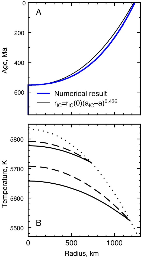
Example of inner core growth history (A) and temperature profiles (B) for a calculation assuming a CMB heat flow equal to 1.15 times the isentropic value, that is 15.3 TW for the present time, with the M & G compositional model. The inner core growth is found to follow a power law with age $τ$ with a power close to 1/2 (thin black line on A). Profiles of conduction temperature in the inner core (solid lines on B) are generally found to be less steep than the isentropic ones (dashed). The liquidus profile (dotted) is computed as a function of the inner core size and varies due to both pressure and composition.

Using the parameters listed in Table 1, equation (13) gives a maximum age for thermal convection equal to 209 Myr. This age can be converted into a CMB heat flow value of 40 TW. Alternatively, since this criterion is approximate, the heat flow across the CMB can be increased so that the present temperature profile would make the inner core neutrally buoyant. Since the inner core always evolves toward stability, even when starting unstably stratified (Deguen and Cardin, 2011), it would mean that the inner core would always have been unstably stratified. This happens for a CMB heat flow always equal to 2.2 times the isentropic value, 29 TW at present and an inner core age equal to 276 Myr. This value for the CMB heat flow is unreasonably high considering the energy balance of the mantle (Jaupart et al., 2007). For a more reasonable heat flow, the temperature in the inner core is always sub-isentropic, as shown in Fig. 1.

The recent upward revision of the thermal conductivity of the core implies that the CMB heat flow must be larger than previously thought for the dynamo to be convectively driven, at least using the conventional buoyancy sources. This favors the possibility of inner core convection since it implies a smaller inner core age than previously envisioned (Gomi et al., 2013). However, because the thermal conductivity increases with depth in the core and with the lesser amount of impurities in the inner core than in the outer one, the minimum requirements for thermal convection in the inner core are much higher than the minimum requirements for convection in the outer one, even without considering the effect of the vast difference in viscosity. The strong stability implied by the type of temperature profile shown in Fig. 1 needs to be overcome by a compositional instability for convection to occur in the inner core.

4 Compositional stratification

The decrease with time (inner core growth) of the ICB temperature from both pressure and composition evolution leads to a change in the partition coefficient (Gubbins et al., 2013). Fig. 2 shows the decrease of the partition coefficient K^sl for S and O with inner core growth as well as the change of mass fraction of both elements in the liquid and the solid, for the two compositional models of the Earth core proposed by Gubbins et al. (2013). The general trends are qualitatively similar for both models and the results differ only quantitatively. On the other hand, the behavior is different between S and O: while the mass fraction of O decreases with radius in the inner core, making it prone to destabilization, the mass fraction of S decreases first before increasing. It appears that in the case of O the effect of the change in the partition coefficient is dominant for the range of inner core size relevant to the Earth, while the effect of the increasing amount of S in the outer core dominates at large inner core sizes. Overall, the stratification in $ξ_{S}$ will tend to make the inner core stable while that in $ξ_{O}$ is adverse.

Fig. 2
(Colour online). Evolution of the partition coefficient of S and O at the ICB (in the mass fraction sense, A, B), mass fraction of S and O in the liquid (C, D) and mass fraction of S and O in the solid (E, F) as a function of the inner core radius for the two compositional models of Gubbins et al. (2013): M & G model (A, C, E) and PREM model (B, D, F). Results for S are represented in blue with the axis on the left and for O in green with the axis on the right. Dotted lines are the variations predicted by leading-order development, which gives a $r_{IC}^{2}$ dependence for the partition coefficients and a $r_{IC}^{3}$ dependence for the concentration in the liquid. Dashed curves are obtained using the same parameterization as Gubbins et al. (2013) for the concentration of S in the outer core and for the liquidus temperature.

In order to understand this difference in behaviors, it is useful to compute the leading-order variations of the concentration and of the partition coefficient. In the case of O, equation (7) provides the necessary expression, which gives:

\frac{δ ξ_{O}^{l}}{ξ_{O0}^{l}} = \frac{r_{IC}^{3}}{r_{OC}^{3} (1 - \frac{3 r_{OC}^{2}}{5 L_{ρ}^{2}})} \equiv A_{O} r_{IC}^{3} .

(14)

In the case of S, assuming that, to leading order, the difference of composition across the ICB $Δ ξ_{S}^{ICB}$ is constant, one gets:

\frac{δ ξ_{S}^{l}}{ξ_{S 0}^{l}} = \frac{Δ ξ_{S}^{ICB}}{ξ_{S0}} \frac{r_{IC}^{3}}{r_{OC}^{3} (1 - \frac{3 r_{OC}^{2}}{5 L_{ρ}^{2}})} \equiv A_{S} r_{IC}^{3} .

(15)

For the partition coefficient, assuming a negligible effect of the variation of concentrations gives, from equation (8),

P_{X}^{sl} = exp (\frac{Δ μ}{k_{B} T_{L}}) ≃ exp (\frac{Δ μ}{k_{B} T_{L_{0}}}) (1 + \frac{Δ μ}{k_{B} T_{L_{0}}} \frac{δ T}{T_{L_{0}}}),

(16)

where

Δ μ = μ_{0}^{l} - μ_{0}^{s} + λ_{X}^{l} C_{X 0}^{l} - λ_{X}^{s} C_{X 0}^{s}

is the initial difference in chemical potential. The change of temperature is, from equation (9), dominated by the pressure term, which gives

\frac{δ P_{X}^{sl}}{P_{X}^{sl}} = \frac{Δ μ}{k_{B} T_{L_{0}}} \frac{K_{0}}{T_{L_{0}}} {(\frac{\partial T_{L}}{\partial P})}_{ξ} \frac{r_{IC}^{2}}{L_{ρ}^{2}} \equiv - B_{X} r_{IC}^{2},

(17)

where the minus sign has been introduced in order to make the coefficient B_X positive, since

Δ μ < 0

Assuming that the logarithmic change of $K_{X}^{sl}$ is equal to that of $P_{X}^{sl}$ , we get for the change of concentration in the solid as function of inner core radius:

\frac{δ ξ_{X}^{s}}{ξ_{X 0}^{s}} = - B_{X} r_{IC}^{2} + A_{X} r_{IC}^{3} .

(18)

This equation shows that the decrease should dominate at small r_IC, while the concentration should increase at large r_IC. The switch of the two effects happens for

r_{IC} = 2 B_{X} / 3 A_{X} \equiv r_{IC}^{⋆}

and the values of the different coefficients and

r_{IC}^{⋆}

are listed in Table 2 for both compositional models. The predictions from this leading-order development are represented by dotted lines in Fig. 2 and show a very good agreement with the full model in the case of O and a qualitatively good agreement in the case of S. The value of

r_{IC}^{⋆}

matches relatively well the full numerical result in the case of S but cannot be tested in the case of O, since it is larger than the core radius. Alternatively, Table 2 provides values of the coefficients fitted to the full numerical results.

Coefficient	M & G model	PREM model	M & G fit	PREM fit
A_O (10^–11 km^–3)	2.696	2.696	2.696	2.696
A_S (10^–11 km^–3)	1.158	0.884	0.835	0.687
B_O (10^–8 km^–2)	14.51	14.66	13.88	13.85
B_S (10^–8 km^–2)	0.837	0.696	0.811	0.532
$r_{IC,O}^{⋆} (km)$	3588	3625	3433	3426
$r_{IC,S}^{⋆} (km)$	482	525	647	517

Several implications need to be drawn from the results presented on Fig. 2. First, O and S have very different behaviors. In the case of O, the large value of $Δ μ_{0}$ (Table 1) makes the partition coefficient vary more strongly with temperature than the partition coefficient for S, by 1.5 orders of magnitude. On the other hand, since the partition coefficient is much smaller for O than for S, the increase of the concentration in the liquid is larger for O than for S, but only by a factor of 3 to 4. Therefore, while both effects balance for an inner core about half its present size in the case of S, the effect of the decrease in the partition coefficient dominates up to the inner core present size in the case of O. Even though O is much less present in the inner core, it is more likely to make the inner core convect. This contrasted behavior is found for both compositional models, which only differ quantitatively.

It is difficult to compare with precision the present results to that of Gubbins et al. (2013), since they do not provide profiles of concentrations in the same way as here and show their results as the evolution of the Rayleigh number with the inner core radius. Nevertheless, their result is qualitatively similar to the ones presented here in the case of the PREM model, with the concentration in S starting as destabilizing and then stabilizing while the concentration in O is always destabilizing. On the other hand, they find that both O and S are always destabilizing in the case of the M & G model, opposite to what is shown in Fig. 2. The reason for this difference in behavior is not clear. A calculation including the approximate evolution of $C_{S}^{l}$ assumed by Gubbins et al. (2013) and neglecting the effect of composition on the evolution of the liquidus temperature was performed, and the results are shown as dashed lines in Fig. 2. The results are rather similar to the results obtained with the full model and the small difference comes mostly from the evolution of the liquidus temperature. In particular, the approximate solution of Gubbins et al. (2013) for the evolution of the concentration of S in the liquid appears rather good. This means that the qualitative differences between the present results and those from Gubbins et al. (2013) in the case of the M & G model cannot be explained by the differences in the treatment of conservation of the solute. Note however that the leading-order analytical calculation presented above are qualitatively similar to the results of the full model, for both compositional models, and gives them support.

Note that, since no compositional diffusion is considered in the inner core (which maximizes the chances of convection), the composition profile depends only on the inner core radius and not on any detail of its growth rate. As explained in section 3, the situation is different for the thermal stratification and the combined thermal-compositional buoyancy requires to consider the time evolution of the core.

5 Combined buoyancy profiles and conditions for a unstable stratification

For a reasonable CMB heat flow, the inner core has been found to be stably stratified in the thermal sense. For the composition, the situation is less clear, with the concentration in O unstably stratified, while the concentration in S is potentially unstable in the innermost part, but stable in the outer part. The combined effect of both compositions and temperature can be estimated by computing the density anomaly with respect to the value at the ICB:

\frac{δ ρ (r)}{ρ_{ICB}} = - α [T (r) - T_{a} (r)] + β_{S} [ξ_{S} (r) - ξ_{S_{f}}] + β_{O} [ξ_{O} (r) - ξ_{O_{f}}],

(19)

with T_a(r) the isentropic temperature profile,

ξ_{X_{f}}

the mass fraction of X at the top of the inner core,

β_{X}

the corresponding expansion coefficient and

α

the coefficient of thermal expansion (see Table 1 for parameter values). The stratification is potentially unstable if the gradient

\partial δ ρ / \partial r > 0

. Whether or not instability indeed occurs in the case where this condition is fulfilled depends on ill-constrained properties (diffusivities, viscosity) that all enter the Rayleigh number, but it is first necessary to consider the sign of the stratification.

Fig. 3 shows the different contributions, temperature and concentration in O and S, to the vertical gradient of the buoyancy, as defined in equation (19). The thermal part depends on the growth rate of the inner core, and the case presented here corresponds to the calculation presented in section 3.

Fig. 3
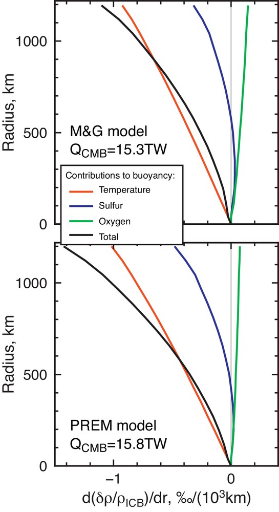
(Colour online). Vertical gradient of the buoyancy and its different contributions for the two compositional models. The CMB heat flow evolution is the same as that used to get Fig. 1, always equal to 1.15 times the isentropic value and 15.3 TW and 15.8 TW at present in the M & G and PREM models, respectively.

It appears that, even though the concentration of O is always destabilizing, its contribution to buoyancy is smaller than that of S. The coefficient of chemical expansion is larger (in absolute sense) for O than for S (Table 1), but the amount of O in the inner core is much smaller and so is its variation as a function of radius. For this reason, the destabilizing effect of O cannot overcome the stabilizing effect of S. The resulting compositional buoyancy is stabilizing in the case of the PREM model and nearly neutral in the case of the M & G model. The larger ICB density jump proposed in the latter model than in PREM requires a larger amount of O in the core and maximizes the importance of the destabilizing oxygen compared to the stabilizing sulfur. Note however that this density jump is on the high end of all proposals for this poorly constrained parameter (Hirose et al., 2013). Middle-of-the-road values are closer to the PREM number or even lower and would suggest a larger effect of S. In any case, it appears that compositional buoyancy is not a very good candidate to set the inner core in motion, at least within the standard outer core model. Since thermal buoyancy is strongly stabilizing, inner core convection seems hard to sustain. Modifications of the standard scenario discussed above need to be considered, however, to completely rule it out. Some possibilities are mentioned in the next section.

6 Discussion and conclusions

The results presented above show that for any reasonable CMB heat flow, the thermal stratification is strongly stabilizing and that the compositional stratification is at best neutral, at least when considering an equilibrium between the inner-core side of the ICB and the bulk of the outer core, an alternate view being presented below. But first, it is worth emphasizing that the choices of thermal conduction parameters have been pushed systematically downward in order to give convection the maximum chances. The values of the conductivity parameters listed in Table 1 correspond to Si being the only light element in the core (Gomi et al., 2013). Using a combination of S and O, as done for other aspects of this paper, would make the central value of conductivity $k_{0} \sim 215 W/m/K$ (Gomi et al., 2013), for the concentration assumed in the liquid. An even larger value should be expected in the inner core, since it contains less solute. Pozzo et al. (2014) give a conductivity at the center equal to 237W/K/m in that case. With this value, a CMB heat flow 3.7 times larger than the isentropic (49 TW at present) value is necessary to make the inner core unstably stratified everywhere, corresponding to an inner core age equal to 185 Myr. Such a high CMB heat flow is clearly excluded and convection in the inner core with such high thermal conductivity is impossible with a well mixed outer core.

The composition of the core is still largely unknown and only two models have been considered above. These models were chosen because all the parameters needed to compute the evolution have been provided by previous studies (Gubbins et al., 2013). It is quite possible that other choices of composition could change the results, although probably not enough to change completely the outcome. Another element, Si, is commonly considered as a possibility in the core. Alfè et al. (2002) have computed equilibrium parameters and found no discernable partitioning at the ICB. This means that Si is not a good candidate to provide the buoyancy needed for inner core convection. On the other hand, since S is found to be stabilizing, if Si were considered in place of S in the core, as it is an option to explain the density both for the inner core and the outer core (Alfè et al., 2002), it could result in a more unstable situation. In order to estimate this effect, I ran some calculations where Si replaces S, keeping the same concentration but using the proper parameters and, in particular, a partition coefficient always equal to 1 and $β_{Si} = - 0.91$ (Deguen and Cardin, 2011). Since the M & G model is the most likely to promote instability, I use these concentrations and just replace S by Si. The resulting buoyancy distribution is shown in Fig. 4. Note that although the molar fraction of Si changes neither in the outer core nor in the inner core, since the partition coefficient is equal to 1 and no expulsion results from the inner core growth, the evolution of the concentration of O makes the mass fraction in Si evolve (Appendix A). However, the resulting buoyancy is negligible. The resulting total buoyancy is strongly stabilizing for a reasonable CMB heat flow.

Fig. 4
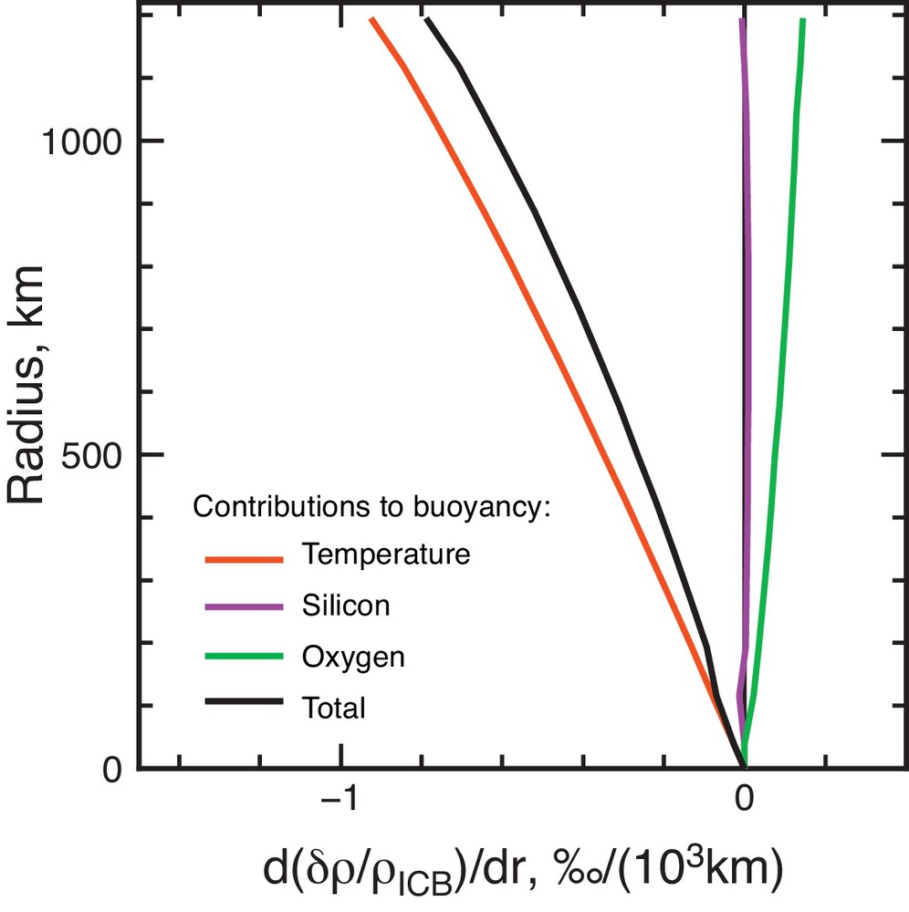
(Colour online). Final buoyancy in the case of a Fe–O–Si core composition with a partition coefficient equal to 1 for Si. The CMB heat flow is assumed to be equal to 1.15 times the isentropic value and equal to 15.3 TW at present.

The analysis presented above is based on the assumption that the outer core is compositionally well mixed, which forms the basis of all classical models of core dynamics and evolution. However, there are some seismological evidences in favor of a compositional stratification both at the base of the outer core (the now called F-layer, e.g. Song and Helmberger, 1995; Souriau and Poupinet, 1991) and at its summit (e.g., Helffrich and Kaneshima, 2010; Tanaka, 2007). Alboussière et al. (2010) proposed to explain the F-layer by a laterally varying melting/freezing boundary condition at the ICB, owing to the translation of the inner core. In this case, the equilibrium condition represented by equation (8) applies to the liquid adjacent to the inner core, not to the bulk of the outer core and both the model of Alboussière et al. (2010) and the condition of stability of the F-layer argue for a liquid concentration at the ICB lower than that of the bulk. If the formation of the F-layer results from the crystallization of the inner core, the increasing concentration in S and O of the bulk of the outer core would not affect the concentration in the crystallizing solid and its evolution would be dominated by the decrease of the partition coefficient. However, if the F-layer formation mechanism requires a convective instability, it is not clear how this process can ever start.

Alternatively, the evolution of the solute concentration of the outer core can be affected by several processes occurring at the top of the core. For example, barodiffusion can act to concentrate light elements in a stably stratified layer at the top of the core (Fearn and Loper, 1981; Gubbins and Davies, 2013). In this case, the concentration of the bulk outer core in light elements is decreased compared to the case where light elements are assumed to stay well mixed. Buffett et al. (2000) also proposed that some of the light elements contained in the core could sediment on its top, which would lead to the same effect. The outcome of the competition between the solute concentration increase due to inner core growth and the decrease from barodiffusion or sedimentation is not settled, but variations of the concentration in solute of the liquid just adjacent to the inner core may not follow from the simple mass balance considered in previous sections.

In order to get an idea of the importance of such effects, the concentration in the liquid can be assumed to be constant with time, meaning that either all the solute-rich fluid released at the ICB by inner core growth is transported across the F-layer without changing its composition or the flux of solute at the top of the core toward the mantle or a stably stratified layer exactly balances the flux from the inner core growth.

Fig. 5 shows the results of such calculations in terms of the different contributions to the buoyancy distribution. The bottom panel uses the same CMB heat flow history than the calculations performed above, Q_CMB = 1.15Q_S. Compared to the cases presented in section 5, both O and S provide a destabilizing buoyancy, but this is still not sufficient to make the total density structure unstably stratified. In order to get neutrally buoyant, the CMB heat flow must be 1.7 times the isentropic value, that is 22.6 TW at present, as can be seen on the top panel of Fig. 5. This value would imply that the mantle is essentially not cooling, which contradicts observations from basalt chemistry (Jaupart et al., 2007).

Fig. 5
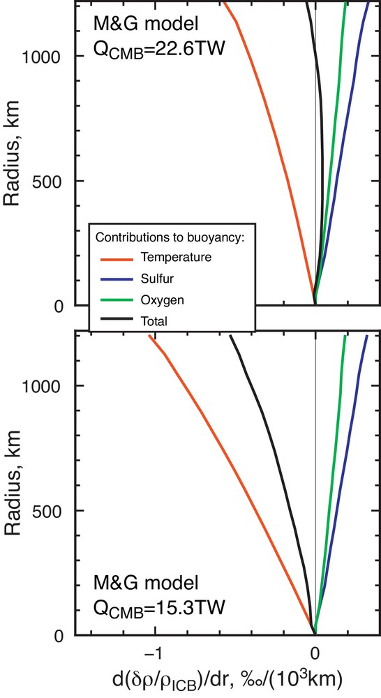
(Colour online). Buoyancy distribution assuming the concentration of the outer core does not vary with inner core growth (see text for details). The bottom panel is obtained for a CMB heat flow 1.15 times larger than the isentropic value (15.3 TW at present), while the top panel is obtained for a CMB heat flow 1.7 times larger than the isentropic value (22.6 TW at present).

Note that if the concentration in solute at the bottom of the outer core is kept constant with time, the decrease of the liquidus temperature with time is lessened compared to the case where the outer core is assumed well mixed. This decreases the effect of temperature on the partition coefficient and this explains why density stratification is not made more dramatically unstable.

For compositional convection to occur in the inner core, it appears that the concentration of solutes at the bottom of the outer core must decrease with time. The mechanism proposed by Alboussière et al. (2010) may allow that, but requires inner core convection, possibly in the form of translation. The density stratification computed in various cases here appears stable for reasonable values of the CMB heat flow. However, because of the vast difference between thermal and chemical diffusivities, double-diffusive instabilities might still be possible (Turner, 1973). However, as pointed out by Pozzo et al. (2014), the timescale for the growth of this instability is the thermal diffusion one and is similar to the age of the inner core. This option might still be the last remaining chance for convection in the inner core and needs to be tested in the future.

Acknowledgments

Suggestions from Renaud Deguen, discussions with Marine Lasbleis, Thierry Alboussière, Yanick Ricard, Dario Alfè and reviews by Chris Davies and Bruce Buffett were very helpful in preparing this paper.

Appendix A Mass and molar fraction.

Depending on the context, molar or mass fraction of any light element is used. Specifically, molar fractions are used by Gubbins et al. (2013) for their model of chemical equilibrium at the ICB, but mass fraction are more convenient for the thermal evolution model (e.g., Braginsky and Roberts, 1995; Labrosse, 2003). Expressions to go from one system to the other are provided here.

Let x_i denote the mole fraction of element i (molar mass M_i) in the mixture, its molar concentration is $C_{i} = x_{i} ρ / M$ , with $ρ$ the density of the mixture and $M = \sum_{i} x_{i} M_{i}$ the average molar mass. The mass fraction of element i is $ξ_{i} = x_{i} M_{i} / M$ . For a mixture of N species, only N – 1 independent fractions define the composition. Considering, as Gubbins et al. (2013), a tertiary mixture of Fe, S and O, the mass fractions in S and O simply write as:

ξ_{O} = \frac{x_{O} M_{O}}{x_{O} M_{O} + x_{S} M_{S} + (1 - x_{O} - x_{S}) M_{Fe}},

(20)

ξ_{S} = \frac{x_{S} M_{S}}{x_{O} M_{O} + x_{S} M_{S} + (1 - x_{O} - x_{S}) M_{Fe}} .

(21)

Inversion of this set of equations leads expressions of $x_{i}$ as functions of $ξ_{i}$ :

x_{O} = \frac{ξ_{O} M_{S} M_{Fe}}{(ξ_{O} M_{S} + ξ_{S} M_{O}) M_{Fe} + (1 - ξ_{O} - ξ_{S}) M_{O} M_{S}},

(22)

x_{S} = \frac{ξ_{S} M_{O} M_{Fe}}{(ξ_{O} M_{S} + ξ_{S} M_{O}) M_{Fe} + (1 - ξ_{O} - ξ_{S}) M_{O} M_{S}} .

(23)

Bibliographie

[Alboussière et al., 2010] T. Alboussière; R. Deguen; M. Melzani Melting-induced stratification above the Earth's inner core due to convective translation, Nature, Volume 466 (2010), pp. 744-747

[Alfè et al., 1999] D. Alfè; M.J. Gillan; G.D. Price The melting curve of iron at the pressures of the Earth's core from ab initio calculations, Nature, Volume 401 (1999), pp. 462-463

[Alfè et al., 2002] D. Alfè; M.J. Gillan; G.D. Price Composition and temperature of the Earth's core constrained by combining ab initio calculations and seismic data, Earth Planet. Sci. Lett., Volume 195 (2002), pp. 91-98

[Alfè et al., 2007] D. Alfè; M.J. Gillan; G.D. Price Temperature and composition of the Earth's core, Contemp. Phys., Volume 48 (2007), pp. 63-80 | DOI

[Braginsky and Roberts, 1995] S.I. Braginsky; P.H. Roberts Equations governing convection in Earth's core and the geodynamo, Geophys. Astrophys. Fluid Dyn., Volume 79 (1995), pp. 1-97

[Buffett, 2009] B.A. Buffett Onset and orientation of convection in the inner core, Geophys. J. Int., Volume 179 (2009), pp. 711-719 | DOI

[Buffett et al., 2000] B.A. Buffett; E.J. Garnero; R. Jeanloz Sediments at the top of Earth's core, Science, Volume 290 (2000), pp. 1338-1342

[Cottaar and Buffett, 2012] S. Cottaar; B. Buffett Convection in the Earth's inner core, Phys. Earth Planet. In., Volume 198–199 (2012), pp. 67-78

[Crank, 1984] J. Crank Free and moving boundary problems, Oxford University Press, Oxford, UK, 1984 (425 p.)

[de Koker et al., 2012] N. de Koker; G. Steinle-Neumann; V. Vlček Electrical resistivity and thermal conductivity of liquid Fe alloys at high P and T, and heat flux in Earth's core, Proc. Natl. Acad. Sci. U.S.A., Volume 109 (2012), pp. 4070-4073

[Deguen, 2012] R. Deguen Structure and dynamics of Earth's inner core, Earth Planet. Sci. Lett., Volume 333–334 (2012), pp. 211-225 | DOI

[Deguen and Cardin, 2011] R. Deguen; P. Cardin Thermochemical convection in Earth's inner core, Geophys. J. Int., Volume 187 (2011), pp. 1101-1118 | DOI

[Deguen et al., 2013] R. Deguen; T. Alboussière; P. Cardin Thermal convection in Earth's inner core with phase change at its boundary, Geophys. J. Int., Volume 194 (2013), pp. 1310-1334 | DOI

[Dziewonski and Anderson, 1981] A.M. Dziewonski; D.L. Anderson Preliminary reference Earth model, Phys. Earth Planet. In., Volume 25 (1981), pp. 297-356

[Fearn and Loper, 1981] D.R. Fearn; D.E. Loper Compositional convection and stratification of Earth's core, Nature, Volume 289 (1981), pp. 393-394

[Gomi et al., 2013] H. Gomi; K. Ohta; K. Hirose; S. Labrosse; R. Caracas; M.J. Verstraete; J.W. Hernlund The high conductivity of iron and thermal evolution of the Earth's core, Phys. Earth Planet. In., Volume 224 (2013), pp. 88-103 | DOI

[Gubbins and Davies, 2013] D. Gubbins; C. Davies The stratified layer at the core-mantle boundary caused by barodiffusion of oxygen, sulphur and silicon, Phys. Earth Planet. In., Volume 215 (2013), pp. 21-28 | DOI

[Gubbins et al., 2013] D. Gubbins; D. Alfè; C.J. Davies Compositional instability of Earth's solid inner core, Geophys. Res. Lett., Volume 40 (2013), pp. 1084-1088 | DOI

[Gubbins et al., 2003] D. Gubbins; D. Alfè; G. Masters; G.D. Price; M.J. Gillan Can the Earth's dynamo run on heat alone?, Geophys. J. Int., Volume 155 (2003), pp. 609-622

[Helffrich and Kaneshima, 2010] G. Helffrich; S. Kaneshima Outer-core compositional stratification from observed core wave speed profiles, Nature, Volume 468 (2010), pp. 807-810

[Hirose et al., 2013] K. Hirose; S. Labrosse; J.W. Hernlund Composition and state of the core, Ann. Rev. Earth Planet. Sci., Volume 41 (2013), pp. 657-691 | DOI

[Jaupart et al., 2007] C. Jaupart; S. Labrosse; J.C. Mareschal, Elsevier (2007), pp. 253-303 (chap. 6)

[Jeanloz and Wenk, 1988] R. Jeanloz; H.R. Wenk Convection and anisotropy of the inner core, Geophys. Res. Lett., Volume 15 (1988), pp. 72-75

[Labrosse, 2003] S. Labrosse Thermal and magnetic evolution of the Earth's core, Phys. Earth Planet. In., Volume 140 (2003), pp. 127-143

[Labrosse, 2014] S. Labrosse Thermal evolution of the core with a high thermal conductivity, Phys. Earth Planet. Inter. (2014) (In preparation)

[Labrosse et al., 2001] S. Labrosse; J.P. Poirier; J.L. Le Mouël The age of the inner core, Earth Planet. Sci. Lett., Volume 190 (2001), pp. 111-123

[Lister and Buffett, 1995] J.R. Lister; B.A. Buffett The strength and efficiency of the thermal and compositional convection in the geodynamo, Phys. Earth Planet. In., Volume 91 (1995), pp. 17-30

[Masters and Gubbins, 2003] G. Masters; D. Gubbins On the resolution of density within the Earth, Phys. Earth Planet. In., Volume 140 (2003), pp. 159-167

[Mizzon and Monnereau, 2013] H. Mizzon; M. Monnereau Implication of the lopsided growth for the viscosity of Earth's inner core, Earth Planet. Sci. Lett., Volume 361 (2013), pp. 391-401 | DOI

[Morelli et al., 1986] A. Morelli; A.M. Dziewonski; J.H. Woodhouse Anisotropy of the inner core inferred from PKIKP travel times, Geophys. Res. Lett., Volume 13 (1986), pp. 1545-1548 | DOI

[Nimmo, 2007] F. Nimmo, Elsevier (2007), pp. 253-303 (chap. 2)

[Poupinet et al., 1983] G. Poupinet; R. Pillet; A. Souriau Possible heterogeneity of the Earth's core deduced from PKIKP travel times, Nature, Volume 305 (1983), pp. 204-206

[Pozzo et al., 2012] M. Pozzo; C.J. Davies; D. Gubbins; D. Alfè Thermal and electrical conductivity of iron at Earth's core conditions, Nature, Volume 485 (2012), pp. 355-358

[Pozzo et al., 2014] M. Pozzo; C. Davies; D. Gubbins; D. Alfè Thermal and electrical conductivity of solid iron and iron-silicon mixtures at Earth's core conditions, Earth Planet. Sci. Lett., Volume 393 (2014), pp. 159-164 | DOI

[Song and Helmberger, 1995] X. Song; D.V. Helmberger A P wave velocity model of Earth's core, J. Geophys. Res., Volume 100 (1995), pp. 9817-9830 | DOI

[Souriau and Poupinet, 1991] A. Souriau; G. Poupinet The velocity profile at the base of the liquid core from PKP(BC + Cdiff) data: An argument in favour of radial inhomogeneity, Geophys. Res. Lett., Volume 18 (1991), pp. 2023-2026 | DOI

[Takehiro, 2011] S.I. Takehiro Fluid motions induced by horizontally heterogeneous Joule heating in the Earth's inner core, Phys. Earth Planet. In., Volume 184 (2011), pp. 134-142 | DOI

[Tanaka, 2007] S. Tanaka Possibility of a low P-wave velocity layer in the outermost core from global SmKS waveforms, Earth Planet. Sci. Lett., Volume 259 (2007), pp. 486-499 | DOI

[Turner, 1973] J.S. Turner Buoyancy Effects in Fluids, Cambridge University Press, Cambridge, 1973 (368 p.)

[Weber and Machetel, 1992] P. Weber; P. Machetel Convection within the inner-core and thermal implications, Geophys. Res. Lett., Volume 19 (1992), pp. 2107-2110

[Woodhouse et al., 1986] J.H. Woodhouse; D. Giardini; X.D. Li Evidence for inner core anisotropy from free oscillations, Geophys. Res. Lett., Volume 13 (1986), pp. 1549-1552 | DOI

[Yukutake, 1998] T. Yukutake Implausibility of thermal convection in the Earth's solid inner core, Phys. Earth Planet. In., Volume 108 (1998), pp. 1-13 | DOI

Commentaires - Politique

Ces articles pourraient vous intéresser

F-layer formation in the outer core with asymmetric inner core growth

Renaud Deguen; Peter Olson; Evan Reynolds

C. R. Géos (2014)

Deformation of directionally solidified alloys: Evidence for microstructural hardening of Earth's inner core?

Michael I. Bergman; Yahya Al-Khatatbeh; Daniel J. Lewis; ...

C. R. Géos (2014)

The inner core and the geodynamo

Stéphane Labrosse; Mélina Macouin

C. R. Géos (2003)