

1 Introduction
The world's environment is in a transition phase and one of the major concerns of today's world is climatic change due to natural as well as to anthropogenic influences. Climatic change can be described as a decadal or even longer period of variation in weather condition (Beg et al., 2002). The major reason is an excessive emission of greenhouse gases, etc., which leads the warming effect (Gadgil and Dhorde, 2005). Among all climatic elements, the key parameter in studying the climatic change is temperature and precipitation brought by urbanization and industrialization. Under the rising temperature scenario expressed in many research papers, mountain areas, especially snow- and glacier-dominated ones, are more vulnerable to the impact of climatic change (Aitken, 2013; Wang et al., 2014). The importance of snow- and glacier-dominated mountains is very well known due to their major role in providing fresh water to large population (Barnett et al., 2005; Bradley et al., 2006; Singh and Bengtsson, 2004). The enhanced melting of snow and glacier may initially increase runoff in the rivers, but at the latter stage, the lack of a glacial buffer ultimately will cause a decrease in water availability, especially during stream-flow periods in the dry season (Bradley et al., 2006), affecting drinking water supply, agriculture, ecosystems, and hydropower. These changes have multiple effects on the other drivers in the society, and have large impact especially on mountain communities as well as on downstream populations. All these challenges have further impacts on regional, social, environmental, and economic systems (Eriksson et al., 2009), whereas they make uncertain future water supply, storage, and hazards, like flood (Orlove et al., 2008). In view of the importance of air temperature and of the availability of a long-term temperature record in the Naradu glacier basin of Himachal Pradesh, an attempt has been made to understand the warming trend in last two and a half decades in this region. The annual and seasonal temperature variations have also been analysed in order to understand the trend.
2 Method and material
2.1 Study area
The study is focussed on Naradu glacier, which is situated in the High Himalayan mountain system of Kinnaur district, Himachal Pradesh. The higher Himalayan regions are most vulnerable to even a slight change in temperature because of the sensitivity of snow and glacier. The impact of the temperature rise can be observed in the form of a migration of species and human beings. A temperature rise also affects biodiversity, economy, and the livelihood of the community. The study is undertaken on the Naradu glacier, which is located in the upper reaches of Naradu Garang Valley, enclosed by high mountain peaks, namely Khimsung (5600 m), Khomsung (5700 m), and Khimloga (5400 m) in the south and southeast of the valley (Koul and Ganjoo, 2010). The glacier is one among the 89 glaciers of Baspa basin, which contributes its water to river Baspa, a tributary of Satluj River. The glacier ranges between 78°22′38.49′′–78°25′57.02′′E and 31°16′27.02′′–31°18′33.57′′N. According to the recent study based on field observation and satellite imagery (LISS-IV, 2011), Naradu glacier covers an area of 3.7 km2. The glacier ranges in altitude from 4512 to 5600 m asl. The location map of the glacier is shown in Fig. 1.
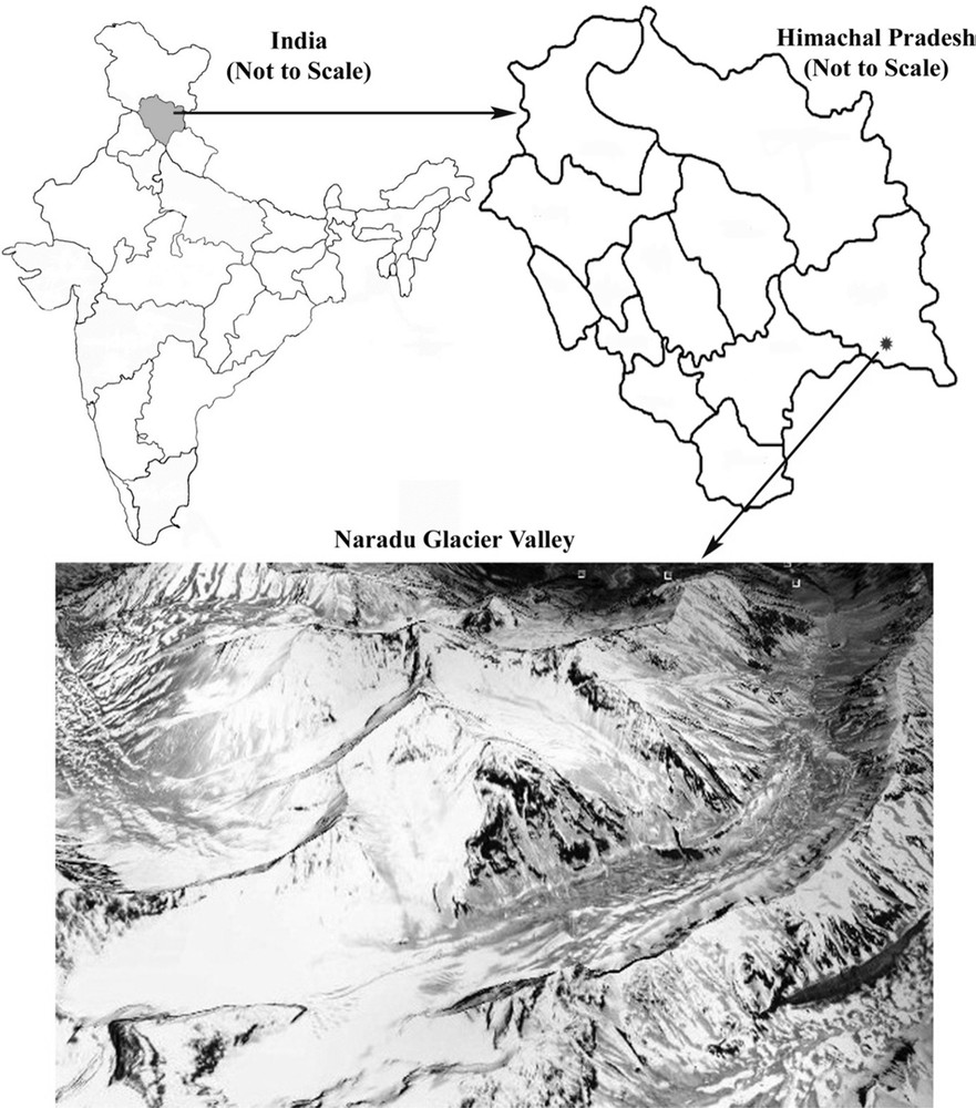
Location map of Naradu glacier, Kinnaur district, Himachal Pradesh (India).
2.2 Data description
The maximum and minimum temperature records are available for the period from 1985 to 2009 on the website of GIOVANNI1 (http://gdata1.sci.gsfc.nasa.gov/daac-bin/G3/gui.cgi?instance_id=MERRA_HOUR_3D) for the glaciated region of Naradu valley, Kinnaur District, Himachal Pradesh. “GIOVANNI” is the acronyms of Geospatial Interactive Online Visualization And aNalysis Infrastructure (Goddard Earth Sciences Data Information Services Center, 2013).
The data has been downloaded by selecting an area of interest, a rectangular block of 31°06′–31°30′N and 78°12′–78°37′E with a grid size of 0.12° × 0.12° in the world's map. Every 3-hourly (UTC) instantaneous upper air temperature data at a pressure level of 600 hPa, resembling that at the altitude of the Naradu glacier, has been downloaded, which includes latitude, longitude, and temperature in Kelvin degrees for the selected point of the grid. This study has utilized MERRA (Modern-Era Retrospective Analysis for Research and Applications), three-hourly 3D data that are a NASA reanalysis for the satellite era using a major new version of the Goddard Earth Observing System Data Assimilation System, Version 5 (GEOS-5). This focuses on historical analyses of the hydrological cycle on a broad range of weather and climate time scales and places the NASA EOS suite of observations in a climate context (NASA GIOVANNI, 2013). The three-hourly (maximum, minimum and mean) data for the entire period have been utilized to compute daily data, and further the daily data have been used to compute the monthly one. The major part of the analysis has been done on a monthly, seasonal, and annual database to understand the temperature trend and its anomalies during different parts of the year.
2.3 Methodology
For the seasonal analysis, the data have been divided into four seasons, like winter (December–February), pre-monsoon (March–May), monsoon (June–September), and post-monsoon (October–November). The monthly data were averaged to provide annual and seasonal values for each year. The data were passed through the Mann–Kendall test (Kendall, 1975; Mann, 1945), along with few other statistical approaches for trend deduction. Assessing the quality of the data is a necessary step. All the data have been checked for outliers, since outliers play a key role in parametric tests and in assessing the magnitude of the possible changes by computing means (moments) and linear regression (Darshana and Pandey, 2013; Eischeid et al., 1995; Feng et al., 2004; Grant and Leavenworth, 1972; Peterson et al., 1998; Takahashi et al., 2011; Xu and Ignatov, 2014). As there were no data gaps, so the gap filling method was not required. Different statistical tools for trend detection have been applied to know the temperature pattern over the period from 1985 to 2009.
The Mann–Kendal approach requires the data to be serially independent. If the data are positively serially correlated, then, the Mann–Kendal approach by itself tends to overestimate the significance of a trend. On the other hand, if the data have a negative serial correlation, then, the significance of the trend is underestimated. Hence, to solve the issue of autocorrelation, the Trend-Free Pre-Whitening (TFPW)-MK procedure proposed by Yue et al. (2002) can be used. Initially, the autocorrelation test was performed to all time series data for checking randomness ascertained by computing autocorrelations for data values at varying time-lags (Modarres and da Silva, 2007). As all lag 1 serial correlation coefficients were statistically not significant (Haan, 2002), there was no need to pre-white the data, and all statistical tests described above are applied to the original time series (Luo et al., 2007).
2.3.1 Autocorrelation test of independence
The first-order autocorrelation coefficient is especially important, because physically the dependence of systems on values in the past is likely to be the strongest for the most recent past. This test is based on values of the correlation coefficients calculated from all pairs of data points separated by k time periods, where k is the lag time. Such autocorrelation coefficients between consecutive values of the same variable are called autocorrelation coefficients. The lag 1 serial correlation coefficient (Wallis and O’Connell, 1972) of annual temperature series was estimated using the equation given below at the 5% significance level for a two-tailed test.
The first order autocorrelation coefficient r1 can be tested against the null hypothesis using Anderson's (1941) limit for the two-tailed test:
2.3.2 Mann–Kendall Test
The Mann–Kendall test, also called Kendall's tau test, is a rank-based non-parametric test for assessing the significance of a trend and has been widely used by many researchers in meteorological and data analysis (Aesawy and Hasanean, 1998; Darshana and Pandey, 2013; Gocic and Trajkovic, 2013; Goossens and Berger, 1986; Hamed and Ramachandra Rao, 1998; Kadioglu, 1997; Mitchel et al., 1966; Tayanc and Toros, 1997). The principal benefit of using the Mann–Kendall test is that it can even be applied to the data series, which is not normally distributed (Hamed, 2009). It is based on the test statics S, defined as
A very high positive value of ‘S’ is an indicator of an increasing trend, whereas a very low negative value indicates a decreasing trend:
It has been documented that when n ≥ 10, the statistic S is approximately normally distributed with the mean E(S) = 0, and its variance is
The standardized test statistic Z is computed as follows:
The null hypothesis, H0, which assumes that there is no significant trend is present and will be rejected if is greater than Zα/2, where α represents the chosen significance level.
2.3.3 Spearman Rank Correlation (SRC) test
In the SRC test, the test statistic is based on the Spearman Rank Correlation coefficient r:
The null hypothesis implying no trend will not be rejected if tν,α/2 < t < tν,1−α/2, where the test statistic t follows a Student's t distribution with degrees of freedom ν = n–2 and significance level α.
2.3.4 Sen's Slope (SS)
Using the method of Sen (1968), the magnitude of the slope can be obtained as follows:
2.3.5 Sequential Mann–Kendall's test
Trend detection study helps in understanding the beginning of change as well as the duration of changes over the entire period covered by the database through Sequential MK (SQMK) test (Modarres and Sarhadi, 2009; Sneyers, 1990). The progressive and retrograde analyses of the Mann–Kendall test will produce sequential values u(t) and u′(t), respectively. These are standardized variables with zero mean and unit standard deviation. So, its sequential behaviour fluctuates around the zero level. The first step in this method is to find out nj, the number of times when Xj > Xi, where Xi and Xj are the sequential values in a series. Xj (j = 1, …, n) are compared with Xi (i = 1,…, j). The test statistic tj of the SQMK test is calculated as:
The mean and variance of the test statistic tj are:
After that, u(tj) is calculated using:
In the same way, u′(tj) is calculated starting from the end of the series.
3 Results
3.1 Preliminary analysis
GIOVANNI's temperature data of Naradu location for the period from 1985 to 2009 were individually analysed. Different statistical factors, like mean, standard deviation, skewness, and kurtosis of the annual mean temperature have been computed.
The annual minimum temperature has shown a variation from –3.89 to –1.73 °C, and the annual maximum temperature varied from –1.40 to 0.2 °C, while the annual mean temperature ranges from –2.5 to –0.5 °C. Standard deviation of maximum and minimum temperature varied from 4.60 to 5.50 °C and 4.77 to 6.05 °C, respectively, while for annual mean temperature data, it varied from 4.61 to 5.73 °C over the 25 years studied.
The skewness test is a measurement of asymmetry in a frequency distribution around the mean. The skewness helps in the selection of statistical tests that can be applied when the data are not normally distributed. Skewness has been calculated for maximum, minimum, and mean temperature, which varied from –0.17 to 0.33 °C, from –0.38 to 0.35 °C, and from –0.38 to 0.24 °C, respectively. The skewness is positive for 80% of the time in the case of maximum temperatures, and for 56% and 64% of the time for minimum and mean temperatures, respectively. Kurtosis, a statistic parameter describing the peakedness of a symmetrical frequency distribution, varied from –1.70 to –1.21 °C, from –1.62 to –0.87 °C and from –1.58 to –1.04 °C, respectively for maximum, minimum, and mean temperatures.
3.2 Analysis of temperature anomalies
Temperature anomalies, i.e. the difference from the normal trend, have been analysed for a better understanding of the variations in the maximum, minimum and mean temperatures for the period extending from 1985 to 2009. The positive anomaly was found to be about 60% of the time for maximum and minimum temperature, while it represented 66% of the time for the annual mean temperature. The change in temperature trend is shown in Figs. 2–4 for annual maximum, minimum, and mean temperatures, respectively. A noticeable warming trend has been observed for the maximum temperature (Fig. 2). The linear trend line in Fig. 2 clearly indicates that the maximum temperature has increased by 1.41 °C. The average maximum temperature till 1997 was sub-zero and shifted towards the positive side since 1998, except for 2002 and 2005. These years (2002 and 2005) have shown the lower temperature and this may be because of increased snow precipitation, which caused high albedo and decreased the temperature. The annual minimum temperature (Fig. 3) has shown an increase of 1.63 °C, while that of the annual mean temperature was 1.49 °C (Fig. 4). It is very evident from the comparisons that night temperature is increasing at a faster rate than day temperature. This would be critical for the locations of higher Himalayas that contain large reserves of snow and ice for freshwater supply. This may enhance the melting rate followed by more discharge and by diminishing the size of the glacier, and will adversely impact freshwater availability in the region and downstream.
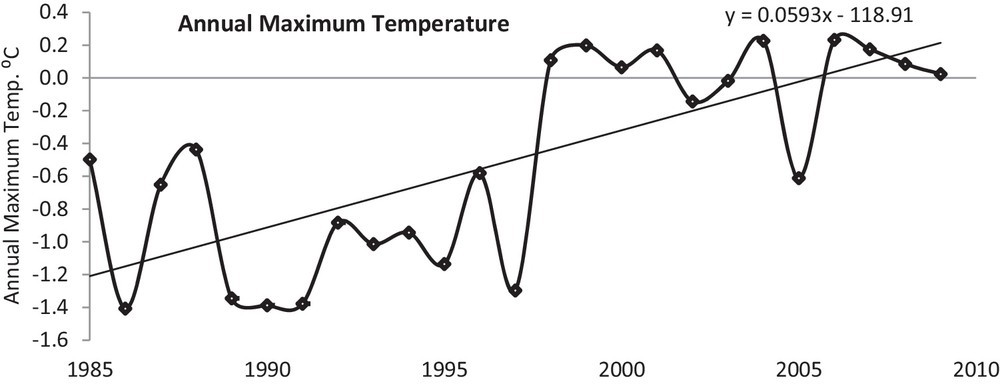
Annual maximum temperature in Naradu valley from 1985 to 2009.
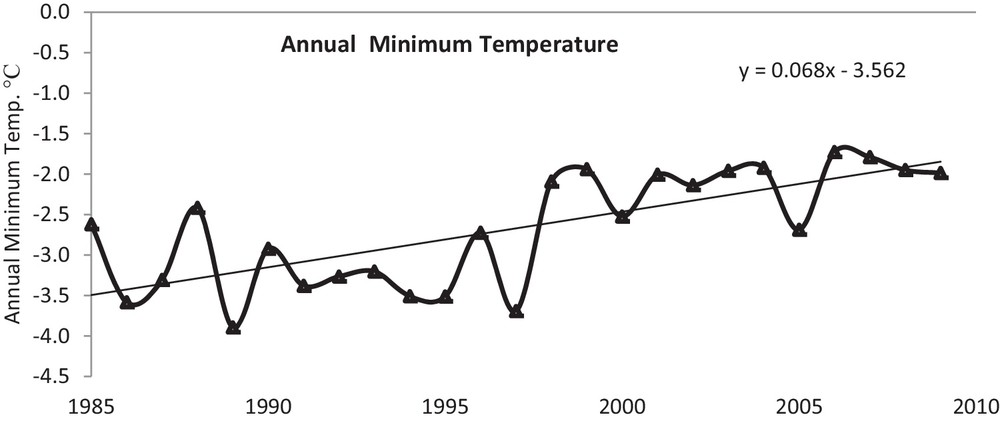
Annual minimum temperature in Naradu valley from 1985 to 2009.
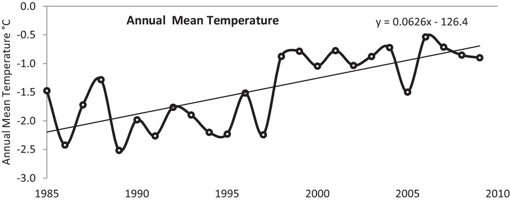
Annual mean temperature in Naradu valley from 1985 to 2009.
The data were also used for seasonal analysis in order to observe the impact of the season on the temperature pattern. To have a quick look at the seasonal and annual warming trend, the data are presented in graphical form (Fig. 5). This clearly shows the warming trend in the annual as well as seasonal minimum temperatures. However, the winter season is showing the highest warming in minimum temperatures, reflecting the overall warming in the valley, with more emphasis on winter warming.
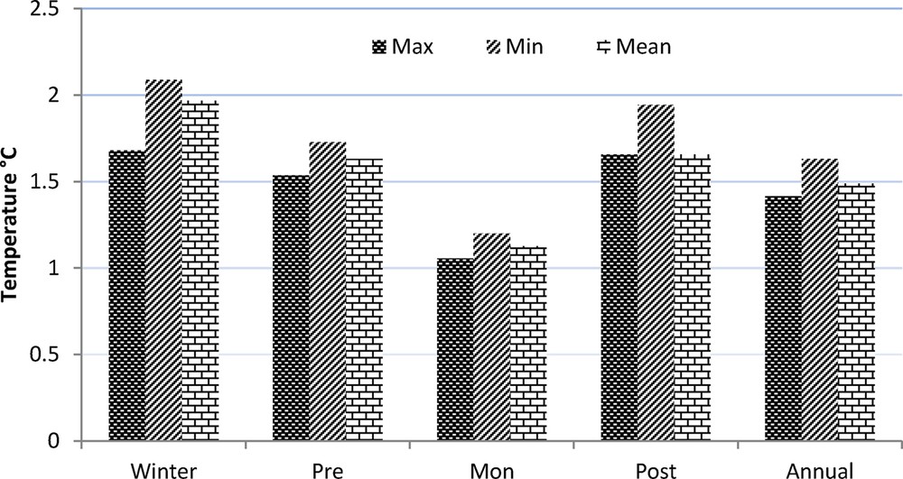
Annual and seasonal temperature anomaly (winter: December–February; pre-monsoon: March–May; monsoon: June–September; post-monsoon: October–November) during 1985-2009.
3.3 Four-yearly variations of annual and seasonal temperature
To ascertain whether the warming rate was uniform for the entire period of analysis or whether there were fluctuation in the warming, the four-yearly temperature variation was analysed on annual and seasonal bases for the maximum, minimum, and mean air temperatures (Table 1) and also compared with data for the entire period (1985–2009). The temperature is negative for all the seasons, except winter, for the period 1985–1989. The period from 1990 to 1994 shows little warming in all the cases, except the minimum temperature. It is very interesting to note that the period 1995–1999 exhibits a high warming trend in all the seasons and for all the temperatures, with a highest of 3.2 °C in the post-monsoon time. The period from 2000 to 2004 shows an interesting cooling trend in winter and post-monsoon, while a warming is evidenced in pre-monsoon and monsoon. The period from 2005 to 2009 shows a warming trend in almost all the cases, except winter. Looking at the complete table, it is evident that the period 1995–1999 really impacts the entire record and pushes the overall trend towards warming. The reason for higher warming in this period is not known, but would be interestingly investigated in the future, with more information on the valley together with meteorological observations, if available.
Four-yearly variations of temperature variables over Naradu glacier.
| Interval | T max | T min | T mean | ||||||||||||
| A | W | Pre-Mon | Mon | Post-Mon | A | W | Pre-Mon | Mon | Post-Mon | A | W | Pre-Mon | Mon | Post-Mon | |
| 1985–1989 | –0.30 | 0.26 | –0.78 | –0.38 | –1.45 | –0.55 | 0.42 | –1.01 | –0.46 | 0.04 | –0.42 | 0.21 | −0.89 | −0.42 | −0.35 |
| 1990–1994 | 0.50 | 0.26 | 0.14 | 0.14 | 3.8 | –0.40 | –1.28 | –0.67 | 0.11 | 0.29 | 0.05 | –0.22 | 0.26 | 0.12 | 1.09 |
| 1995–1999 | 1.34 | 1.68 | 1.62 | 0.46 | 3.2 | 1.51 | 0.67 | 1.64 | 0.45 | 1.10 | 1.42 | 1.44 | 1.63 | 0.46 | 1.35 |
| 2000–2004 | 0.05 | –0.72 | 0.66 | 0.02 | –2.18 | 0.50 | –0.99 | 1.28 | 0.08 | –0.74 | 0.28 | −0.92 | 0.97 | 0.05 | −0.92 |
| 2005–2009 | 0.45 | –0.01 | 0.72 | 0.18 | 1.48 | 0.47 | –1.22 | 0.76 | –0.03 | 0.94 | 0.46 | −0.20 | 0.61 | 0.08 | 0.84 |
| 1985–2009 | 1.41 | 1.67 | 1.54 | 1.06 | 1.66 | 1.63 | 2.09 | 1.73 | 1.20 | 1.94 | 1.49 | 1.97 | 1.63 | 1.13 | 1.88 |
3.4 Results of Mann–Kendall, Spearman rank correlation, Sen's Slope and Sequential Mann–Kendall test and linear regression test over the Naradu glacier
MK, SRC, and SS tests have been applied to Naradu glacier for the period from 1985 to 2009 for three categories, viz., Tmax, Tmin, and Tmean. The linear regression test was also used to evaluate the monthly, annual and seasonal long-term changes in air temperature over the entire Naradu glacier. Apart from this, the linear trend fitted with the data was also tested with Student's t-test to verify the results obtained by MK and SRC tests; the results are presented in Tables 2 and 3. The results of all the tests reveal the significant increasing trend of minimum, maximum and mean temperature in almost all months.
Results of Mann–Kendall statistical tests for monthly and seasonal temperature variables over the period 1985 to 2009.
| Month | T max | T min | T mean | ||||||
| Z | Liner equation | Cal. t | Z | Liner equation | Cal. t | Z | Liner equation | Cal. t | |
| January | 2.873* | y = 0.056x – 7.898 | 3.169539* | 2.032* | y = 0.080x – 10.87 | 2.093072* | 2.406* | y = 0.068x – 9.384 | 2.509853* |
| February | 1.471 | y = 0.041x – 7.313 | 1.728786** | 1.331 | y = 0.062x – 10.52 | 1.28517 | 1.425 | y = 0.051x – 8.917 | 1.489731 |
| March | 1.939** | y = 0.045x – 5.634 | 1.870213** | 1.938** | y = 0.063x – 7.886 | 1.796042** | 1.845** | y = 0.054x – 6.760 | 1.886502** |
| April | 2.312* | y = 0.073x – 2.570 | 2.658074* | 2.125* | y = 0.065x – 4.383 | 2.435327* | 1.985* | y = 0.069x – 3.476 | 2.58407* |
| May | 2.546* | y = 0.076x + 0.381 | 2.702412* | 2.172* | y = 0.087x – 1.990 | 2.628492* | 2.079* | y = 0.081x – 0.804 | 2.768875* |
| June | 3.340* | y = 0.054x + 3.597 | 3.989623* | 3.060* | y = 0.054x + 1.509 | 3.184527* | 3.246* | y = 0.054x + 2.553 | 3.770521* |
| July | 3.246* | y = 0.041x + 6.012 | 3.858921* | 2.359* | y = 0.047x + 3.808 | 3.350551* | 3.06* | y = 0.044x + 4.910 | 3.714835* |
| August | 1.985** | y = 0.026x + 6.143 | 2.352866* | 2.966* | y = 0.045x + 4.011 | 2.961073* | 2.966* | y = 0.036x + 5.077 | 2.813179* |
| September | 2.452* | y = 0.053x + 3.492 | 2.842724* | 3.06* | y = 0.054x + 1.511 | 2.909252* | 2.733* | y = 0.054x + 2.501 | 2.931451* |
| October | 1.752** | y = 0.062x – 1.139 | 2.208798* | 2.452* | y = 0.075x – 2.912 | 2.34534* | 2.359* | y = 0.069x – 2.026 | 2.435327* |
| November | 2.219* | y = 0.087x – 4.186 | 2.754107* | 2.499* | y = 0.086x – 6.109 | 2.961073* | 2.452* | y = 0.087x – 5.147 | 3.057581* |
| December | 1.891** | y = 0.093 x–6.109 | 2.208798* | 2.265* | y = 0.102x – 8.922 | 2.658074* | 2.219* | y = 0.097x – 7.515 | 2.613692* |
| Annual | 3.340* | y = 0.059x – 1.268 | 4.922187* | 3.503* | y = 0.068 x–3.562 | 4.981671* | 3.993* | y = 0.062x – 2.257 | 5.041929* |
| Winter | 2.686* | y = 0.070x – 7.138 | 3.380996* | 2.499* | y = 0.087x – 10.11 | 3.177031* | 3.012* | y = 0.082x – 8.684 | 3.778511* |
| Pre-monsoon | 3.060* | y = 0.064x – 2.607 | 3.289913* | 2.406* | y = 0.072x – 4.753 | 3.312614* | 2.779* | y = 0.068x – 3.680 | 3.388622* |
| Monsoon | 4.181* | y = 0.044x + 4.811 | 5.764956* | 3.993* | y = 0.050 x + 2.710 | 5.072358* | 4.087* | y = 0.047x + 3.761 | 5.578319* |
| Post-monsoon | 1.798** | y = 0.069x – 2.207 | 2.532146* | 2.639* | y = 0.081x – 4.511 | 3.162051* | 2.219* | y = 0.078x – 3.586 | 3.124665* |
Results of Spearman Rank Correlation tests for monthly and seasonal temperature variables over the period 1985 to 2009.
| Month | T max | T min | T mean | |||
| r s | t | r s | t | r s | t | |
| January | 0.534* | 3.026* | 0.404* | 2.119* | 0.444* | 2.379* |
| February | 0.284** | 1.42 | 0.298** | 1.499 | 0.299** | 1.505 |
| March | 0.383* | 1.988** | 0.387* | 2.014** | 0.395* | 2.060** |
| April | 0.489* | 2.685* | 0.467* | 2.533* | 0.460* | 2.487* |
| May | 0.489* | 2.687* | 0.470* | 2.556* | 0.459* | 2.479* |
| June | 0.628* | 3.866* | 0.535* | 3.038* | 0.596* | 3.559* |
| July | 0.639* | 3.983* | 0.506* | 2.813* | 0.597* | 3.573* |
| August | 0.397* | 2.073* | 0.555* | 3.197* | 0.557* | 3.218* |
| September | 0.471* | 2.562* | 0.551* | 3.165* | 0.501* | 2.775* |
| October | 0.430* | 2.282* | 0.521* | 2.927* | 0.526* | 2.967* |
| November | 0.478* | 2.613* | 0.545* | 3.118* | 0.515* | 2.884* |
| December | 0.430* | 2.284* | 0.497* | 2.747* | 0.497* | 2.750* |
| Winter | 0.589* | 3.499* | 0.587* | 3.474* | 0.644* | 4.041* |
| Pre-monsoon | 0.579* | 3.408* | 0.519* | 2.914* | 0.562* | 3.257* |
| Monsoon | 0.788* | 6.138* | 0.715* | 4.904* | 0.779* | 5.964* |
| Post-monsoon | 0.471* | 2.558* | 0.598* | 3.575* | 0.779* | 5.96* |
| Annual | 0.701* | 4.711* | 0.722* | 5.005* | 0.732* | 5.150* |
In the MK test, the analysis of the maximum temperature showed a significant warming trend in all the months, except February, from 1985 to 2009. Using the linear regression test, the monthly rate of change of the maximum temperature varied from 0.62 °C (August) to 2.23 °C (December). A significant increasing trend was observed in annual, winter, pre-monsoon, monsoon and post-monsoon temperatures. It was found from seasonal analysis that the winter maximum temperature showed the maximum increasing rate (1.68 °C) followed by post-monsoon (1.65 °C), pre-monsoon (1.54 °C) and monsoon (1.06 °C) seasons.
Using the MK test, the minimum temperature showed a significant warming trend in all the months, except February, at the 5% and 10% significance level. Using linear trends, the monthly rate of change of the minimum temperature varied from 1.08 °C (August) to 2.45 °C (December) over 25 years. The results reveal a significant increase in annual, winter, pre-monsoon, monsoon, and post-monsoon temperatures. The increase in annual minimum temperature was 1.63 °C from 1985 to 2009 over Naradu glacier. Seasonally, the winter temperature has the maximum increase (2.09 °C), followed by post-monsoon (1.94 °C), pre-monsoon (1.73 °C), and monsoon (1.2 °C) season.
In addition this has also been analysed for the monthly rate of change of mean temperature, which varied from 0.86 °C (August) to 2.33 °C (December). The increase in annual mean temperature was 1.49 °C during the period from 1985 to 2009. Our seasonal analysis shows that winter mean temperature has a maximum increasing rate (1.97 °C) followed by post-monsoon (1.66 °C), pre-monsoon (1.63 °C), and monsoon (1.12 °C) season. The above results suggest that the climate of Naradu glacier is getting warmer, and that warming is more pronounced during night than day.
In SRC test analysis, maximum, minimum and mean temperatures for all the months, except February show a significant increasing trend, which confirms the results obtained from MK test.
Sen's Slope test (Table 4), which gives a magnitude of the slope, also shows an increasing trend for each year and for all the seasons over the period from 1985–2009.
Results of Sen's Slope Statistical tests for monthly and seasonal temperature variables over the period from 1985 to 2009.
| Year (SS°C/month) | Max | Min | Mean | Max | Min | Mean | |
| 1985 | 0.055 | 0.057 | 0.057 | ||||
| 1986 | 0.056 | 0.058 | 0.056 | Winter (SS °C/year) | 0.003 | 0.004 | 0.004 |
| 1987 | 0.066 | 0.050 | 0.075 | Pre-monsoon (SS °C/year) | 0.003 | 0.003 | 0.003 |
| 1988 | 0.061 | 0.068 | 0.063 | Monsoon (SS °C/year) | 0.002 | 0.002 | 0.002 |
| 1989 | 0.050 | 0.069 | 0.064 | Post-monsoon (SS °C/year) | 0.003 | 0.003 | 0.003 |
| 1990 | 0.036 | 0.048 | 0.053 | ||||
| 1991 | 0.048 | 0.066 | 0.057 | Annual (SS °C/year) | 0.002 | 0.003 | 0.003 |
| 1992 | 0.059 | 0.075 | 0.069 | ||||
| 1993 | 0.052 | 0.064 | 0.069 | ||||
| 1994 | 0.040 | 0.071 | 0.057 | ||||
| 1995 | 0.060 | 0.083 | 0.078 | ||||
| 1996 | 0.066 | 0.079 | 0.074 | ||||
| 1997 | 0.046 | 0.041 | 0.054 | ||||
| 1998 | 0.071 | 0.056 | 0.061 | ||||
| 1999 | 0.057 | 0.066 | 0.062 | ||||
| 2000 | 0.044 | 0.062 | 0.059 | ||||
| 2001 | 0.044 | 0.047 | 0.061 | ||||
| 2002 | 0.045 | 0.063 | 0.056 | ||||
| 2003 | 0.051 | 0.058 | 0.059 | ||||
| 2004 | 0.036 | 0.051 | 0.051 | ||||
| 2005 | 0.078 | 0.066 | 0.069 | ||||
| 2006 | 0.047 | 0.043 | 0.046 | ||||
| 2007 | 0.064 | 0.061 | 0.066 | ||||
| 2008 | 0.064 | 0.075 | 0.079 | ||||
| 2009 | 0.048 | 0.047 | 0.050 |
The SQMK test has been applied to annual and seasonal average temperatures. The graphs show a variety of information, which can be summarized according to the trend/no trend hypothesis that can be accepted at the 5% significance level. When the progressive MK value crosses either of the confidence limit lines, it indicates a significant trend at the 5%-significance level–crossing the upper line implies a significant positive trend (Nalley et al., 2013). In each case, the forward line crosses the confidence line (1.96), hence a different variety of data, i.e. Tmax, Tmin, and Tmean show increasing trends for all the annual and seasonal data. This makes stronger the argument that all the annual and seasonal temperature data follow a positive trend. Figs. 6(a), 7(a) and 8(a) show the progressive and retrograde sequential annual values for the period from 1985 to 2009, where the beginning of the positive trend has been observed after the year 1997. These results are also in agreement with the observation that has been made in the regular plot of the annual maximum, minimum, and mean temperature data (Figs. 2, 3 and 4).
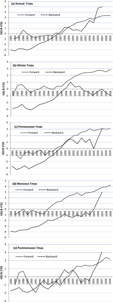
a–e: progressive and retrograde sequential values of maximum temperature at Naradu using SQMK test statistics for annual, winter, pre-monsoon, monsoon, and post-monsoon.
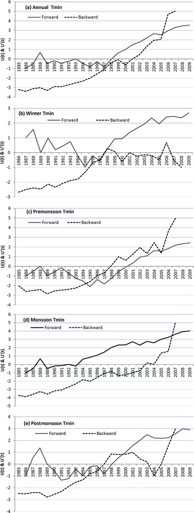
a–e: progressive and retrograde sequential values of minimum temperature at Naradu using SQMK test statistics for annual, winter, pre-monsoon, monsoon, and post-monsoon.
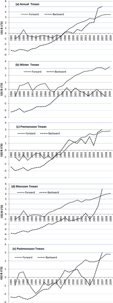
a–e: progressive and retrograde sequential values of mean temperature at Naradu using SQMK test statistics for annual, winter, pre-monsoon, monsoon, and post-monsoon.
4 Discussion
The temperature trends reported by Bhutiyani et al. (2007) and Shrestha et al. (1999) were about 1.6 °C/100 year and 0.03–0.12 °C/year, respectively, in different parts of Himalaya. It was an attempt to understand the temperature change in the region of Naradu glacier and to compare it with temperature changes in different parts of Himalaya.
The selection of the analysis period obviously affects the outcome, as proven when comparing the results based on different periods, but the limitation of the data in the higher Himalayas cannot be ruled out. The larger data series can be better analysed through the analysis of the whole record, and we have taken the annual averages of every three-hourly maximum and minimum temperature from 1985 to 2009. The data were subjected to analysis for even a monthly scale, as well as for the seasonal scale. The most important aspects for the long-term trends in the study region reveal that there are significant increases of 1.41 °C in annual maximum temperature, 1.63 °C in annual minimum temperature and 1.49 °C in annual mean temperature over 25 years in Naradu Valley. These findings are in conformity with the results of studies conducted by several researchers (Heino et al., 1999; Karl et al., 1993; Qiang et al., 2004; Wibig and Glowicki, 2002), which have shown that minimum temperatures have increased more rapidly than the maximum temperatures in different parts of the globe. These results are in agreement with the analysis at several stations of the northern hemisphere, especially European ones, which showed a larger trend for the minimum temperature than for the maximum daily temperature.
Seasonal analysis showed that the magnitudes of the positive trends in winter, post-monsoon, pre-monsoon and monsoon mean temperature were 1.96 °C, 1.66 °C, 1.63 °C and 1.13 °C, respectively. The same pattern has been observed for maximum and minimum temperatures, but night temperature is found to be increasing more rapidly than day temperature. This study is consistent with the one conducted by Bhutiyani et al. (2007) in northwestern Himalaya. An analysis on a monthly time step indicated a significant warming trend in all the months, except February, in mean, minimum, and maximum temperatures during the analysed period from 1985 to 2009.
5 Conclusions
Two and a half decade-long temperature records of the region of Naradu glacier in the High Himalayan Mountain range of Himachal Pradesh have been analysed in detail to demonstrate the observed changes in maximum, minimum, and mean air temperatures. Emphasis was placed on the quantification of temperature change on annual, monthly, and seasonal bases. The analysis indicated that there is an overall warming trend in the valley, more pronounced for minimum temperatures, making warmer winters. The conclusions drawn from the study are listed below.
The annual temperature has increased by 1.41 °C for the maximum, 1.63 °C for minimum, and 1.49 °C for the mean ones.
The trend is positive for all seasons, while it is the largest for winter minimum temperature (2.09 °C), evidencing a warmer winter in the valley.
The seasonal analyses of the mean temperature revealed that the temperature magnitude increased during the period from 1985 to 2009 by 1.97 °C, 1.88 °C, 1.63 °C and 1.13 °C for winter, post-monsoon, pre-monsoon, and monsoon, respectively. In addition, both mean minimum and mean maximum temperatures follow the same trend as the mean annual temperature does. However, the magnitude of the mean minimum temperature variation is little less than 2 °C.
The trends were also examined on a monthly basis, evidencing a significant warming in all the months, except February, for annual mean, minimum, and maximum temperatures from 1985 to 2009 in the valley.
SRC tests were also applied on monthly and seasonal bases, showing a significant positive trend in all the months, except February.
Sens's slope also confirms the results of MK and SRC tests.
A sequential version of the Mann–Kendall test was applied to annual and seasonal data, revealing also a warming trend, whose beginning took place in 1997 in the case of all annual temperature data.
The clear warming trend in the valley will certainly have an impact on the precipitation pattern and on snow and ice melting. Hence, an additional study will be helpful in order to understand the precipitation change as a consequence of temperature change through quantification of discharge, provided that ground data are available for verification.
Acknowledgements
The analyses and visualizations used in this paper were produced by the GIOVANNI online data system, developed and maintained by the NASA GES DISC, hence the authors are thankful to NASA who has provided the online data for helping researchers. Authors would like to acknowledge support from the Department of Science and Technology (DST), Govt. of India, in the form of research project No. SR/DGH/HP-1/2009 dated 09.09.2010 in Naradu Valley, which has incited us to analyze the temperature pattern in the valley apart from the other objectives of the project.
1 GIOVANNI is a web-based application developed by the Goddard Earth Sciences Data and Information Services Centre (GES DISC) that provides a simple and intuitive way to visualize, analyze, and access vast amounts of Earth science remote sensing data without having to download the data.