1 Introduction
Temperature is the second most important meteorological variable after precipitation because it can be related to solar radiation and thus with both evaporation and transpiration processes which constitute an important phase of the hydrologic cycle. IPCC (2007) reported the increasing tendencies in temperature in many areas of the world in space and time. Nicholls and Collins (2006) found that the average maximum temperature in Australia has increased by 0.6 °C from 1910 to 2004 and minimum temperature by 1.2 °C from 1950 to 2004. The increasing trend in monthly and seasonal surface temperature in Europe is warmer in late 20th and early 21st century than that of any time during the past 500 years (Luterbacher et al., 2004). In North America, annual mean air temperature is increased during the period of 1955 to 2005, with the greatest warming in Alaska and northwestern Canada. For Canada as a whole, the annual mean temperature has increased by 1.2 °C over the past 53 years (Vincent et al., 2007).
In Asia, increasing trends have been observed across the seven sub regions of Asia (IPCC, 2007). The observed rise in mean annual temperature is 2 to 3 °C in Russia (Peterson et al., 2002; Savelieva et al., 2000), 1.8 °C in Mongolia (Batima et al., 2005), 0.7 °C in Northwest China (Shi et al., 2002), 1.0 °C in Japan (Ichikawa, 2004), 0.23 °C in Korea (Jung et al., 2002) and 0.14 °C in Philippines (Cruz et al., 2006).
In India also increasing trend is found in the annual mean temperature, annual maximum temperature and annual minimum temperature (Arora et al., 2005; Dash et al., 2007; Kothawale and Rupa Kumar, 2005; Pant and Kumar, 1997; Sinha Ray and De, 2003). Few research studies have been conducted separately on various cities in India (Dhorde et al., 2009; Gadgil and Dhorde, 2005) and found the mix trends in temperature series.
Research studies carried out by various researchers found that the increasing trends in air temperature have been related to several factors such as increased concentrations of anthropogenic greenhouse gases (De and Mukhopadhyay, 1998; Easterling et al., 1997; Qiang et al., 2004; Soltani and Soltani, 2008), increased emissions of anthropogenic aerosols (Cohen and Stahill, 1996; Ramanathan et al., 2007), increased cloud cover and urbanization (Ji and Zhou, 2011; Tabari and Hosseinzadeh Talaee, 2011). Further, IPCC (2007) reported that most of the observed increase in average temperature since the mid-twentieth century is very likely due to the observed increase in anthropogenic greenhouse gas concentrations. The major greenhouse gases (GHGs) are water vapor, which causes about 36–70% of the greenhouse effect; carbon dioxide (CO2), which causes 9–26%; methane (CH4), which causes 4–9%; and ozone (O3), which causes 3–7% (Kiehl and Trenberth, 1997). GHGs warm the surface and the atmosphere with significant implications for rainfall retreat of glaciers and sea ice, sea level, among other factors (Ramanathan and Feng, 2009). The greenhouse effect is the phenomenon where water vapour, CO2, CH4 and other atmospheric gases absorb outgoing infrared radiation, resulting in the raising of the temperature. GHGs absorb and emit long wave radiation, while aerosols absorb and scatter solar radiation (Ramanathan and Feng, 2009).
Ozone is a secondary air pollutant that is formed by the transformation reactions of primary air pollutants, especially nitrogen dioxide (NO2). O3 is one of the major pollutants in the atmosphere, causing several damages on human health, climate, vegetation and materials (Fuhrer et al., 1997; Karnosky et al., 2005; Musselman and Massman, 1999; Ollerenshaw et al., 1999; Smidt and Herman, 2004). Ozone concentration builds up in the atmosphere from several natural and anthropogenic sources. These include:
- • downward transport of stratospheric O3 through the free troposphere to near-ground level;
- • in situ O3 production from methane emitted from swamps and wetlands reacting with natural nitrogen oxides (NOx);
- • production of O3 from reaction of volatile organic compounds (VOCs) with NOx;
- • long-range transport of O3 from distant pollution sources (EPA, 1993; Kondratyev and Varotsos, 2001a, 2001b; Varotsos et al., 2004).
There are several studies reporting the increase of the surface O3 (Bojkov, 1986; Cartalis and Varotsos, 1994; Jaffe et al., 2003; Lee et al., 1998; Lisac and Grubisic, 1991; Nolle et al., 2005; Oltmans et al., 1998; Vingarzan, 2004; Vingarzan and Thomson, 2004). Comparisons of ozone background levels with those measured in the late 19th–early 20th centuries indicate that current ozone levels have risen by approximately two times (Bozo and Weidinger, 1995; Cartalis and Varotsos, 1994; Staehelin et al., 1994). The main factors for high ozone level episodes are the increase of temperature, photolysis reactions of nitrogen oxides and the variation in boundary layer as function of temperature during the day and the night times (Pires et al., 2012).
Under a warmer climate, the arid and semiarid region like MP could experience severe water stress due to the decline in soil moisture. Agriculture is the mainstay of the State's economy as it provides 71% of employment. Since the agricultural productivity is likely to suffer severely due to higher temperatures and no study was found in literature on spatial and temporal variability of temperature at Madhya Pradesh (MP), the aims of this study are:
- • to investigate the spatial and temporal variability of temperature of this region;
- • to examine the relationship of cloud cover with temperature variables;
- • to find the impact of urbanization on temperature.
2 Method and material
2.1 Details of study area
The State of MP is centrally located and is often called the “Heart of India”, comprising a geographical area of 443,000 km2, occupying 14.5% of the area of India. The State is bordered by seven other States: Uttar Pradesh, Bihar, Orissa, Andhra Pradesh, Maharashtra, Gujarat and Rajasthan. The study area extends from 21°17′ N to 26°36′ N and 74°02′ N to 82°26′ E covering 45 districts. MP has a subtropical climate. There are three distinct seasons: summer (March to May), winter (November to February), and the intervening rainy months of the southwest monsoon (June to October). MP experiences extreme temperatures both during summer and winter. In summer, the temperature goes up to 42 °C, and in winter it falls tremendously to 10 °C. The temperature starts rising from March and it starts falling from October. The temperature also varies from place to place in the State. The hottest place is Bhind in summer where the temperature reaches up to 45 °C, while in Bhopal the temperature is closer to 43 °C. The average temperature in winter is around 10 °C. Rainfall increases from west to east and decreases towards north. The State receives maximum rainfall from June to September. Annual average rainfall varied from 694.42 mm in southwest (Westnimar station) part of the MP to about 1417.28 mm in eastern part (Mandla station) (Darshana and Pandey, 2013) of MP. The latitudinal decline in rainfall and longitudinal increase decide the cropping systems that are grown across the State. The cropping patterns in MP change with rainfall; for example, the eastern part of the State is characterized by its rice based cropping systems and the central and western parts of the State have soybean based cropping systems where pulses and oilseed occupy an important place. The State has been delineated into five major crop zones, namely: rice; rice-wheat; wheat; jowar-wheat; cotton-jowar and soybean.
2.2 Data description
Monthly maximum, minimum and mean air temperature and cloud cover (%) data of 45 stations covering a period of 102 years (1901 to 2002) were downloaded from the Indian Meteorological Department (IMD) site India water portal (http://www.indiawaterportal.org/metdata). Population data was collected from the Census of India (2011) publication. Fig. 1 shows the locations of meteorological stations. Data quality control is a necessary step; however, since Mann–Kendall (MK) test is a rank-based nonparametric test, they are robust against outliers. On the other hand, outliers play a key role in parametric tests and in assessing the magnitude of the possible changes by computing means (moments) and linear regression (Darshana and Pandey, 2013). For the present study the data series were plotted to detect the outliers. After visual detection of outliers, the suspected values were calculated using the normal ratio method. As all series were complete, no gap filling method was needed. November, December, January and February were considered for the analysis of winter temperature as these 4 months record the lowest temperatures. While computing the mean for winter season, December of the previous year was included. March, April and May are the months with highest mean maximum temperatures and, therefore, represent the summer season. June to October constitute monsoon season. The monthly data were averaged to provide annual and seasonal values for each year.

Location of the meteorological stations at Madhya Pradesh.
Localisation des stations météorologiques de Madhya Pradesh (MP).
2.3 Methodology
2.3.1 Trend detection
The moving average or running mean is a conventional procedure used to reduce the inter-annual variability of time series (Sneyers, 1992). A 10-year running average was used in the present study. Linear trend represented by the slope of the simple least square regression line provided the rate of rise/fall in the variable. Using the value of the rate of change, the total change over the last 102 years was computed.
Autocorrelation is also called lagged correlation or serial correlation which refers to the correlation of a time series with its own past and future values (Madnani, 2009). In the terminology of the atmospheric sciences, this dependence through time is usually known as persistence (Chattopadhyay et al., 2011). Persistence can be defined as the existence of (positive) statistical dependence among successive values of the same variable, or among successive occurrences of a given event (Wilks, 2006). The short-range correlations are described by the autocorrelation function, which declines exponentially with a certain decay time. However, for the long-range correlations, the autocorrelation function declines as a power-law (Varotsos, 2005b). The direct calculation of the autocorrelation function is usually not appropriate to distinguish among different decay patterns at long lags, due to noise superimposed on the data (Galmarini et al., 2004; Kantelhardt et al., 2002; Stanley, 1999). The detrended fluctuation analysis (DFA), introduced by Peng et al. (1994), is a well-established method for determining the scaling behavior of noisy data in the presence of trends without knowing their origin and shape (Talkner and Weber, 2000). Therefore, the DFA method was used in the present study to check the scaling behavior of monthly air temperatures variable namely maximum, minimum and mean air temperature data over MP.
Nonparametric tests are also referred to as distribution-free tests. These tests have the several advantages over parametric methods. Some of these advantages include:
- • they do not require the assumption of normality or the assumption of homogeneity of variance;
- • they compare medians rather than means and, as a result, if the data have one or two outliers, their influence is negated;
- • prior transformations are not required, even when approximate normality could be achieved;
- • greater power is achieved for the skewed distributions;
- • data below the detection limit can be incorporated without fabrication of values or bias (Helsel, 1987).
The influence of serial correlation in the time series on the results of MK test (Kendall, 1975; Mann, 1945) has been discussed in the literature (Yue et al., 2002). Hence to solve the issue of autocorrelation, the Trend-Free Pre-Whitening (TFPW)-MK procedure proposed by Yue et al. (2002) was used. Lag-1 autocorrelation coefficient (Haan, 2002) was used to detect the presence of serial correlation in data series. The temperature series which were found serially independent, MK test was directly applied to the original sample data. However, the series which were found serially correlated, pre-whitening was used before applying the MK test. Confidence levels of 90% and 95% and 99% were taken as thresholds to classify the significance of positive and negative temperature trends. The brief explanations of methods used are given in the Appendix.
To explore the spatial distribution of trends for temperature variables, the Sen Slope estimator (β) proposed by Sen (1968) was interpolated using ArcGIS 9.3 based on each individual station β value.
2.3.2 Effect of urbanization on temperature
To study the effect of urbanization on temperature, the study period is categorized into two parts; less urbanized period (LUP) and more urbanized period (MUP). The LUP and MUP are identified based on the population trends. Fig. 2 shows that up to 1951 population growth was slow, but after 1951 population growth was fast as compared to 1951. Considering this variation in the growth pattern, the period from 1901 to 1951 is identified as LUP and the period from 1961 to 2001 is characterized by MUP.

Less urbanized period (LUP) and more urbanized period (MUP) at Madhya Pradesh.
Période de moindre urbanisation (LUP) et d’urbanisation plus prononcée (MUP) à Madhya Pradesh.
2.3.3 The relationship of air temperature and cloud cover
The Pearson correlation test is applied to detect the relationship between cloud cover and temperature variables on annual and seasonal basis. The significance of correlation is tested at a 5% significance level using Kendall-tau method.
3 Results and discussion
3.1 Preliminary analysis
The statistical parameters (mean, standard deviation, skewness, kurtosis and coefficient of variation) of the annual mean temperature have been computed for each station. The annual mean temperature in the State varied from 24.34 to 26.61 °C and standard deviation from 0.37 to 0.50 during the 102 years. The skewness, which is a measure of asymmetry in a frequency distribution around the mean, varied from −0.39 to 0.27, predominantly positive skewness, with an average around 0.02 indicating the annual temperature during the period is asymmetric and it lies to the right of the mean over all the stations. Kurtosis, a statistic parameter describing the peakedness of a symmetrical frequency distribution, varied from −0.57 to 0.55. The coefficient of variation (CV), a statistical measure of the dispersion of data points in a data series around the mean, was computed for all stations in order to investigate the spatial pattern of inter-annual variability of annual temperature over the study area. The CV varied from 1.45% (Balaghat district) to 1.99% (Katni district). The average CV of entire MP was 1.6 percent. It can be concluded that the zones of usually higher temperatures are the zones of least variability, and the zones of lowest temperatures are the zone of highest variability.
3.2 Analysis of autocorrelation structure of the monthly air temperature
Koscielny-Bunde et al. (1998) stated that temperature records follow a universal scaling law. This behavior was said to be found in numerous daily and monthly temperature data sets (Eichner et al., 2003; Kiraly et al., 2006; Koscielny-Bunde et al., 1998; Maraun et al., 2004; Talkner and Weber, 2000; Tsonis et al., 2000; Varotsos and Kirk-Davidoff, 2006). In order to test the short and long-range correlation in the monthly temperature series from 1901 to 2002 (n = 1224) at MP, DFA1 was used. The time series is first integrated using Eq. (1) (Appendix) to exaggerate the non-stationarity of the original data, reduce the noise level, and generate a time series corresponding to the construction of a random walk that has the values of the original time series as increments. After that the integrated time series is divided into boxes of equal length d. In each box of length d, a least squares line (or polynomial curve of order 1) is fitted to the data (representing the trend in that box). Further, the integrated time series is detrended using Eq. (2) (Appendix) by subtracting the local trend in each box. The root-mean-square fluctuation of this integrated and detrended time series is calculated and denoted as F(d). This computation is repeated over all time scales (box sizes), from all minimum box size to maximum box size, to characterize the relationship between F(n), the average fluctuation, and n, the box size. The minimum box size used is 2k + 2 (where k is the order of polynomial curve, in this case K = 1) and the maximum box size used is one-tenth of the length of the input series (Ivanov et al., 2001). A log-log plot of the root-mean-square fluctuation function Fd and Δt of the integrated and detrended monthly air temperature series over MP is shown in Fig. 3. Exponents (slope of log-log plot) α of 1.21 (± 0.07), 1.14 (± 0.09) and 1.19 (± 0.08) were found for maximum, minimum and mean air temperature respectively, which indicates that long-range power-law correlations prevail in temperature data over MP. It can be concluded that air temperature over the MP exhibits persistent long-range correlations.

Log-log plot of root-mean-square fluctuation function (F(d)) versus temporal change Δt (in months) over MP for maximum air temperature (a) for minimum air temperature (b) and for mean air temperature (c).
Diagramme log-log de la fonction (F(d)) de fluctuation de la valeur quadratique moyenne en fonction du changement temporel Δt (en mois) sur Madhya Pradesh pour les températures de l’air maximale (a), minimale (b) et moyenne (c).
3.3 Analysis of temperature anomalies
The temperature anomalies have been computed for better understanding of the observed trends in the minimum temperature, the maximum temperature and the mean temperature during the time period of 102 years (1901 to 2002). Figs. 4–6 show the annual temperature anomalies in the maximum, minimum and mean temperature averaged over the MP. A well-marked warming trend is observed in the maximum temperature (Fig. 4). From Fig. 4, it was observed that the anomaly became positive after 1947 and the positive enhancement became sharp till year 2002. The linear trend line indicates that the maximum temperature is increased by 0.60 °C in the last 102 years over MP. Further, the minimum temperature (Fig. 5) also shows the positive anomalies after 1947. The increase in minimum temperature was 0.62 °C during the 102 years. Furthermore, the annual mean temperature showed an increase of 0.60 °C (Fig. 6) over the MP. From the above, it reveals that the night temperature is increasing at faster rate than day temperature.
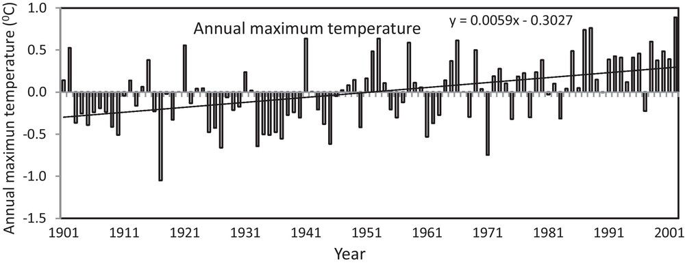
Anomalies in annual maximum temperature at Madhya Pradesh from 1901 to 2002.
Anomalies dans la température maximale annuelle à Madhya Pradesh, sur la période 1901 à 2002.
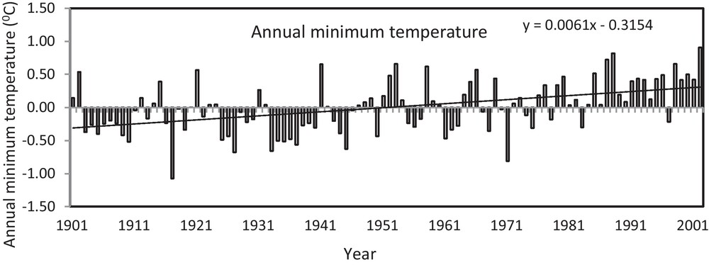
Anomalies in annual minimum temperature at Madhya Pradesh from 1901 to 2002.
Anomalies dans la température minimale annuelle à Madhya Pradesh, sur la période 1901 à 2002.
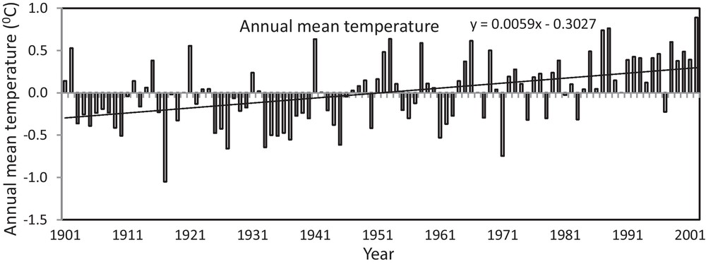
Anomalies in annual mean temperature at Madhya Pradesh from 1901 to 2002.
Anomalies dans la température moyenne annuelle à Madhya Pradesh, sur la période 1901 à 2002.
3.4 Decadal variations of annual and seasonal temperature
To ascertain whether the warming rate was uniform throughout the last century or not, decade-to-decade rates over entire MP were computed. The decadal variation of temperature was studied for the annual and seasonal basis (Table 1) and compared with long-term series (1901 to 2002). In general, for all the temperature variables, episodic variation was noticed and up to 1960s, there is a cooler period of decreasing temperature (Table 1). This period was followed by a warming period. Real warming appears to have started in the decade of 1961 to 1970 with a modest rate and continued till the end of the century. The warming rate appears to be highest during the period from 1971 to 1980 as compared to the other periods. The warming rates are less afterwards, as compared to 1980 in the rest of the decades.
Variation décennale des variables de température sur Madhya Pradesh.
| Decades | T min | T max | T mean | |||||||||
| A | W | S | M | A | W | S | M | A | W | S | M | |
| 1901–1910 | −0.71 | 0.02 | −0.59 | −1.4 | −0.71 | 0.02 | −0.59 | −1.41 | −0.69 | 0.02 | −0.57 | −1.38 |
| 1911–1920 | −0.38 | −0.47 | −0.55 | −0.29 | −0.38 | −0.46 | −0.55 | −0.29 | −0.37 | −0.45 | −0.54 | −0.28 |
| 1921–1930 | −0.60 | −1.11 | −1.56 | 0.05 | −0.60 | −1.12 | −1.56 | 0.05 | −0.59 | −1.09 | −1.52 | 0.05 |
| 1931–1940 | −0.32 | −0.30 | −0.35 | −0.38 | −0.29 | −0.27 | −0.29 | −0.36 | −0.30 | −0.28 | −0.31 | −0.36 |
| 1941–1950 | −0.34 | −0.26 | −0.52 | −0.10 | −0.31 | −0.22 | −0.48 | −0.08 | −0.32 | −0.23 | −0.49 | −0.08 |
| 1951–1960 | −0.31 | 0.44 | −0.41 | −0.58 | −0.25 | 0.60 | −0.32 | −0.59 | −0.28 | 0.51 | −0.36 | −0.57 |
| 1961–1970 | 0.51 | 1.21 | 0.17 | 0.45 | 0.84 | 1.37 | 0.77 | 0.66 | 0.66 | 1.26 | 0.46 | 0.54 |
| 1971–1980 | 0.83 | 1.93 | −0.06 | 0.68 | 0.22 | 1.28 | −0.74 | −0.03 | 0.51 | 1.57 | −0.39 | 0.32 |
| 1981–1990 | 0.49 | 0.83 | 0.74 | −0.11 | 0.45 | 0.98 | 0.82 | −0.39 | 0.46 | 0.88 | 0.76 | −0.24 |
| 1991–2002 | 0.31 | 0.56 | 0.40 | −0.02 | 0.27 | 0.53 | 0.46 | −0.25 | 0.29 | 0.54 | 0.46 | −0.22 |
| 1901–2002 | 0.62 | 1.25 | 0.61 | 0.09 | 0.60 | 1.22 | 0.59 | 0.07 | 0.60 | 1.20 | 0.59 | 0.07 |
The mean minimum temperature anomaly was negative from 1901–1910 to 1951–1960. However, it becomes positive from 1961 to 1970. The highest anomaly was 0.83 °C in 1971 to 1980, which was higher than the anomaly of long-term mean (1901 to 2002). The winter temperature anomaly was negative from 1911–1920 to 1941–1950 decade and positive in 1901 to 1910, 1951 to 1960, 1961 to 1970, 1971 to 1980, 1981 to 1990 and 1991 to 2002. The highest anomaly was 1.93 °C during 1971 to 1980, which is higher than the long-term annual series (1901 to 2002). Further, in summer, the temperature shows a positive anomaly in the 1961 to 1970, 1981 to 1990 and 1991 to 2002 decades, and a negative anomaly during rest of the decades. The inter decadal variation of temperature anomaly in the monsoon season was positive during the 1921 to 1930, 1961 to 1970 and 1971 to 1980 decades, out of which the highest was 0.68 °C in the 1971 to 1980 decade.
The annual maximum temperature anomaly was positive after the decade 1951 to 1960, and the highest in 1961 to 1970 decade (0.84 °C). The winter temperature anomaly was negative in four decades i.e. 1911–1920 to 1941–1950. However, positive anomaly was found in rest of the decades and highest in the decade from 1961 to 1970 (1.37 °C) than the long-term average annual over the analysis period. The summer anomaly was lower than the winter anomaly in all the decades, and had its highest value of 0.82 °C during 1981 to 1990 in comparison to the long-term analysis period. In monsoon, the temperature shows the positive anomaly only in the periods from 1921 to 1930 and 1961 to 1970. The mean temperature anomaly shows the same decadal pattern like minimum and maximum temperatures on the annual and seasonal scales.
3.5 Results of Mann–Kendall test and linear regression test over entire Madhya Pradesh
MK test and linear regression test were used to evaluate the monthly, annual and seasonal long-term changes in air temperature over entire MP. Apart from this, the linear trend fitted to the data was also tested with the Student t-test to verify results obtained by the MK test and results are presented in Table 2. The results of the MK test reveal the significant increasing trend in almost all months of minimum, maximum and mean temperature. The minimum temperature showed the significant warming trend in February, March, April, October, November and December during the analysis period from 1901 to 2002. Using the linear regression test, the month wise rate of change of minimum temperature varied from −0.47 °C (June) to 1.94 °C (November). The significant increasing trend was observed in annual, winter and summer temperatures. It is found from seasonal analysis that the winter minimum temperature showed the maximum increasing rate (1.24 °C) followed by summer (0.61 °C) and monsoon (0.08 °C) season.
Résultats des tests statistiques pour les variables de températures mensuelles, sur la période 1901 à 2002.
| Month | T min | T max | T mean | ||||||
| Z | Linear equation | Calculated “t” | Z | Linear equation | Calculated “t” | Z | Linear equation | Calculated “t” | |
| January | 1.2028 | y = 0.004x + 2.4441 | 1.3147 | 1.1363 | y = 0.0029x + 20.132 | 0.98224 | 1.2867 | y = 0.0031x + 11.699 | 1.03765 |
| February | 3.5679* | y = 0.0131x − 13.363 | 3.9631* | 3.3019* | y = 0.0123x +4.6601 | 3.46606* | 3.5188* | y = 0.0122x − 3.8086 | 3.6179* |
| March | 2.4692* | y = 0.0085x + 0.729 | 2.3061* | 1.9632* | y = 0.0081x + 18.08 | 2.10324* | 2.3333* | y = 0.0082x + 9.1145 | 2.19702* |
| April | 1.7261** | y = 0.0078x + 7.172 | 2.1605* | 1.5845 | y = 0.0076x + 23.539 | 2.02781* | 1.6828** | y = 0.0075x + 14.958 | 2.0852* |
| May | 0.5407 | y = 0.0018x + 22.773 | 0.5203 | 0.5060 | y = 0.0018x + 37.423 | 0.52126 | 0.3007 | y = 0.0018x + 29.324 | 0.537 |
| June | −0.7171 | y = −0.0046x + 35.097 | −0.10511 | −0.9223 | y = −0.0037x + 44.758 | −0.84062 | −0.7518 | y = −0.0035x + 37.986 | −0.84001 |
| July | 0.1099 | y = −0.0017x + 27.271 | −0.64128 | −0.3990 | y = −0.0011x + 33.672 | −0.39291 | −0.0289 | y = −0.001x + 28.884 | −0.36726 |
| August | −0.8154 | y = −0.0005x + 24.232 | −0.32737 | −0.5754 | y = −0.0008x + 31.364 | −0.48466 | −0.7575 | y = −0.0008x + 27.372 | −0.4697 |
| September | 1.2202 | y = 0.003x + 16.362 | 1.56874 | 0.5869 | y = 0.0029x + 25.583 | 1.34334 | 0.9802 | y = 0.003x + 20.218 | 1.53659 |
| October | 2.8740* | y = 0.0081x + 3.1541 | 2.86522* | 2.6485* | y = 0.0089x + 15.023 | 3.17317* | 2.9203* | y = 0.0088x + 7.8967 | 3.20615* |
| November | 5.0281* | y = 0.019x − 23.366 | 5.73994* | 5.1206* | y = 0.0196x − 9.029 | 5.85353* | 5.0252* | y = 0.0192x + 16.433 | 5.8746* |
| December | 5.1813* | y = 0.0151x − 18.905 | 6.08555* | 5.3982* | y = 0.0153x − 3.7642 | 6.32720* | 5.0917* | y = 0.0151x − 11.633 | 6.36376* |
| Annual | 5.0310* | y = 0.0061x + 6.9667 | 5.22818* | 4.5076* | y = 0.0059x + 20.64 | 5.11493* | 4.8806* | y = 0.0059x + 12.974 | 5.29612* |
| Winter | 6.1648* | y =0.0122x − 12.125 | 6.5967* | 5.2698* | y = 0.0119x + 4.1463 | 6.52137* | 6.2587* | y = 0.0118x − 3.9161 | 6.60162* |
| Summer | 2.2929* | y = 0.006x + 10.225 | 2.36017* | 1.8591** | y = 0.0058x + 26.518 | 2.18378* | 2.1541* | y = 0.0058x + 17.969 | 2.27402* |
| Monsoon | 0.6130 | y = 0.0008x + 21.223 | 0.51987 | 1.1941 | y = 0.0007x + 31.25 | 0.74911 | 0.5465 | y = 0.0007x + 25.638 | 0.46019 |
Using the MK test, the maximum temperature showed the significant warming trend in February, March, October, November and December at 5% significance level. Using linear trend the monthly rate of change of the maximum temperature varied from −0.41 (June) to 1.76 (November) °C/102 years. The results reveal the significant increase in annual, winter and summer maximum temperatures. The increase in annual maximum temperature was 0.60 °C from 1901 to 2002 over the MP. Seasonally, the winter temperature has the maximum increase (1.21 °C) followed by summer (0.59 °C) and monsoon (0.07 °C) season.
Further, month wise rate of change of mean temperature varied from −0.36 °C (June) to 1.96 °C (November). The increase in annual mean temperature was 0.60 °C during the analysis period of 1901 to 2002 over the MP. Seasonal analysis shows that the winter mean temperature has the maximum increasing rate (1.20 °C) followed by summer (0.59 °C) and monsoon (0.07 °C) season. The above results suggest that the climate of the MP is getting warmer and warming is more pronounced during night than during day.
3.6 Stations wise trend in annual and seasonal temperature variables
Table 3 shows the results of MK test. The annual maximum, minimum and mean temperature showed a statistically significant increasing trend over all the stations. The seasonal maximum temperature showed a statistically significant increasing trend at all the stations (at 5% significance level) in the winter season, 25 stations (at 5% significant level) in the summer season and eight stations (five stations at 5% significance level and three stations at 10% significance level) in the monsoon season, respectively. The seasonal minimum temperature reveal the statistically significant increasing trend at all the stations in the winter season (at 5% significance level) and 27 stations (19 stations at 5% significance level and eight stations at 10% significance level) in the summer seasons. However, in the monsoon season, it shows the increasing trend in only five stations and the decreasing trend in three stations. Further, the seasonal mean temperature showed a statistically significant trend at 5% significance level at all the stations (increasing) in winter season, 27 stations (increasing) in summer and nine stations (six increasing and three decreasing) in the monsoon season. It is observed that in some stations there is a significant trend at the annual scale but there is a no significant trend at the seasonal scale.
Résultats du test Mann–Kendall dans les séries de températures sur Madhya Pradesh.
| Name of district | T max | T min | T mean | |||||||||
| A | W | S | M | A | W | S | M | A | W | S | M | |
| Balaghat | + | + | + | + | + | + | ||||||
| Barwani | + | |||||||||||
| Betul | + | + | + | |||||||||
| Bhind | + | + | + | |||||||||
| Bhopal | + | + | + | |||||||||
| Chhatarpur | + | − | + | − | + | |||||||
| Chhindwara | + | + | + | + | − | |||||||
| Damoh | + | + | + | + | + | + | ||||||
| Datia | + | − | + | − | + | − | ||||||
| Dewas | ||||||||||||
| Dhar | ||||||||||||
| Dindori | + | + | + | + | + | + | ||||||
| East Nimar | ||||||||||||
| Guna | + | + | + | |||||||||
| Gwalior | − | |||||||||||
| Harda | + | + | + | |||||||||
| Hoshangabad | + | + | + | |||||||||
| Indore | ||||||||||||
| Jabalpur | + | + | + | + | + | + | ||||||
| Jhabua | + | + | + | |||||||||
| Katni | + | + | + | + | + | + | ||||||
| Mandla | + | + | + | + | + | + | ||||||
| Mandsaur | + | + | + | |||||||||
| Morena | + | + | + | |||||||||
| Narsimhapur | + | + | + | + | + | + | ||||||
| Neemuch | − | + | − | |||||||||
| Panna | + | + | + | + | + | + | ||||||
| Raisen | + | + | + | |||||||||
| Rajgarh | + | + | + | |||||||||
| Ratlam | + | + | + | |||||||||
| Rewa | + | − | + | − | + | − | ||||||
| Sagar | + | + | + | + | ||||||||
| Satna | + | − | + | − | + | − | ||||||
| Sehore | + | + | + | |||||||||
| Seoni | + | + | + | + | + | + | ||||||
| shahdol | + | + | + | + | + | + | ||||||
| Shajapur | + | + | + | |||||||||
| Sheopur | − | − | − | |||||||||
| Shivpuri | − | − | − | |||||||||
| Sidhi | + | − | + | + | + | − | ||||||
| Tikamgarh | − | − | − | |||||||||
| Ujjain | + | + | + | |||||||||
| Umaria | + | + | + | + | + | + | ||||||
| Vidisha | + | + | + | |||||||||
| Westnimar |
3.7 Spatial distribution of temporal change in temperature
Exploring long-term changes in temperature patterns is one of the important components in climate change analysis. Using spatial analysis more insight into local and regional trends of climate pattern can be provided for better understanding of climate (Boyles and Raman, 2003). In this study, β was used instead of the least squares estimate because it is less sensitive to the non-normality of the distribution and less affected by extreme values or outliers in the series (Zhang et al., 2000). An inverse distance weighted interpolation method (IDW), which is based on the assumption that the interpolation surface should be influenced most by nearby points and less by more distant points (Gemmer et al., 2004) was used. A variable search radius with a minimum sample of 12 points was used. To control the significance of the surrounding point on the interpolated value the exponent of distance (power) four was used because the higher power results in less influence from distant points. The spatial distributions of the temperature variable on annual and seasonal bases are shown in Figs. 7–18.
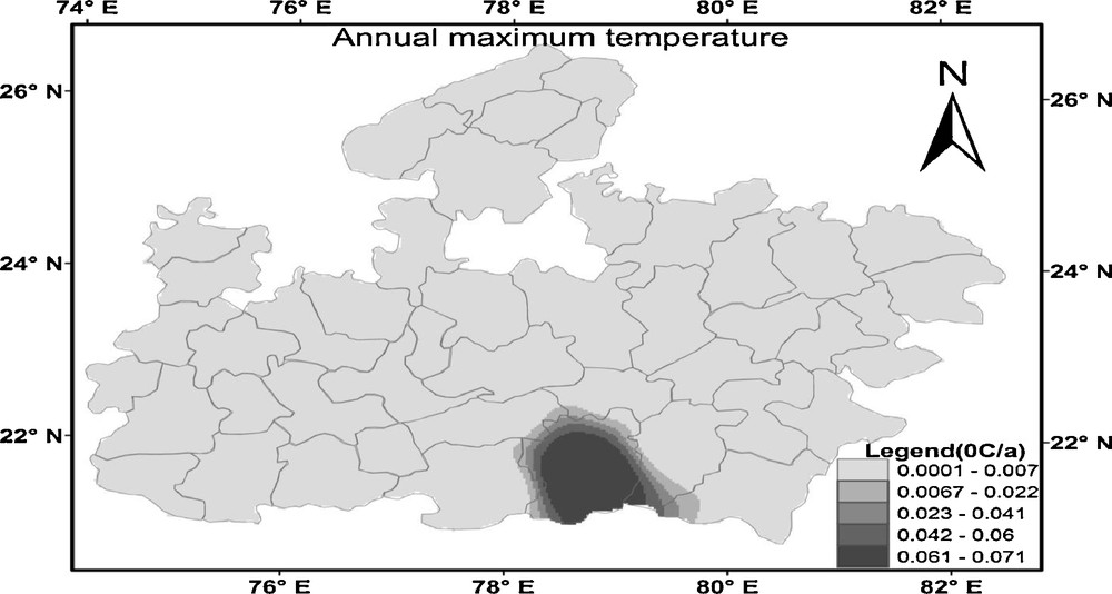
Spatial distribution of temporal change in annual maximum temperature at MP from 1901 to 2002.
Distribution spatiale du changement temporel dans la température maximale annuelle à Madhya Pradesh, sur la période 1901 à 2002.
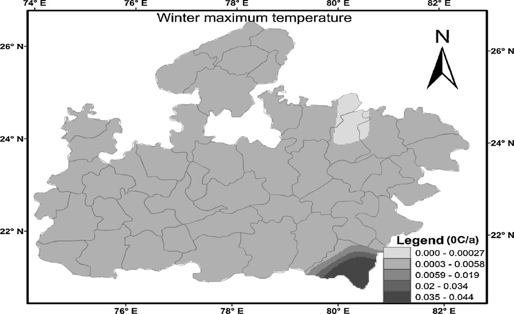
Spatial distribution of temporal change in winter maximum temperature at Madhya Pradesh from 1901 to 2002.
Distribution spatiale du changement temporel dans la température maximale d’hiver à Madhya Pradesh, sur la période 1901 à 2002.
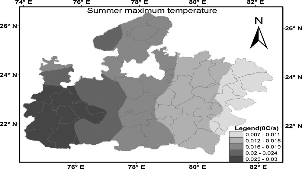
Spatial distribution of temporal change in summer maximum temperature at Madhya Pradesh from 1901 to 2002.
Distribution spatiale du changement temporel dans la température maximale d’été à Madhya Pradesh, sur la période 1901 à 2002.
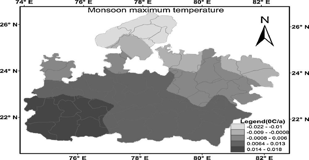
Spatial distribution of temporal change in the monsoon maximum temperature at Madhya Pradesh from 1901 to 2002.
Distribution spatiale du changement temporel dans la température maximale de mousson à Madhya Pradesh, sur la période 1901 à 2002.
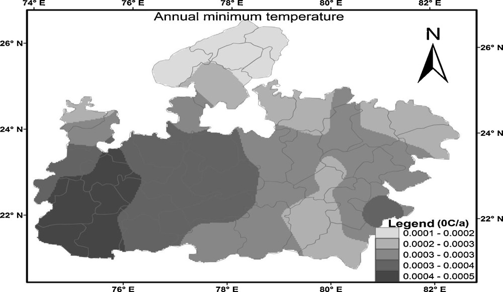
Spatial distribution of temporal change in the annual minimum temperature at Madhya Pradesh from 1901 to 2002.
Distribution spatiale du changement temporel dans la température minimale annuelle à Madhya Pradesh, sur la période 1901 à 2002.
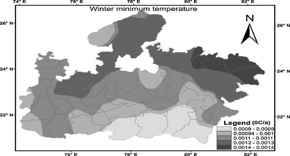
Spatial distribution of temporal change in the winter minimum temperature at Madhya Pradesh from 1901 to 2002.
Distribution spatiale du changement temporel dans la température minimale d’hiver à Madhya Pradesh, pour la période 1901 à 2002.

Spatial distribution of temporal change in the summer minimum temperature at Madhya Pradesh from 1901 to 2002.
Distribution spatiale du changement temporel dans la température minimale d’été à Madhya Pradesh, pour la période 1901 à 2002.
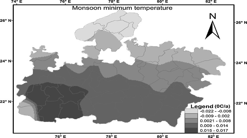
Spatial distribution of temporal change in the monsoon minimum temperature at Madhya Pradesh from 1901 to 2002.
Distribution spatiale du changement temporel dans la température minimale de mousson à Madhya Pradesh, sur la période 1901 à 2002.

Spatial distribution of temporal change in the annual mean temperature at Madhya Pradesh from 1901 to 2002.
Distribution spatiale du changement temporel dans la température moyenne annuelle, à Madhya Pradesh, sur la période 1901 à 2002.
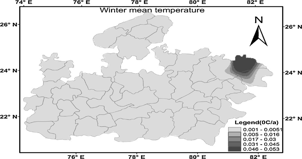
Spatial distributions of temporal change in winter mean temperature at Madhya Pradesh from 1901 to 2002.
Distribution spatiale du changement temporel dans la température moyenne d’hiver à Madhya Pradesh, sur la période 1901 à 2002.
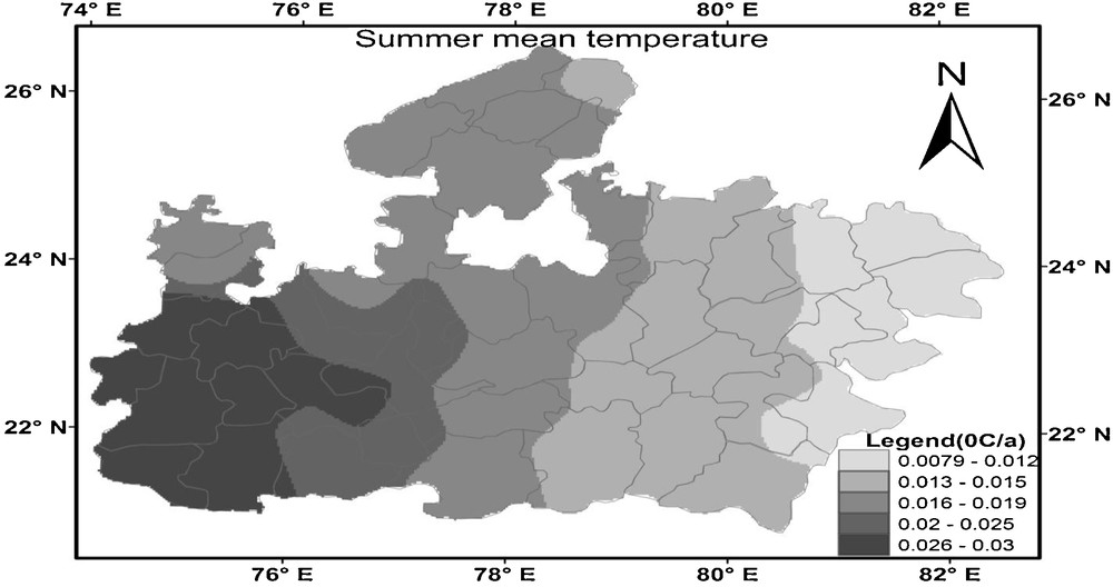
Spatial distributions of temporal change in summer mean temperature at Madhya Pradesh from 1901 to 2002.
Distribution spatiale du changement temporel dans la température moyenne d’été à Madhya Pradesh, sur la période 1901 à 2002.
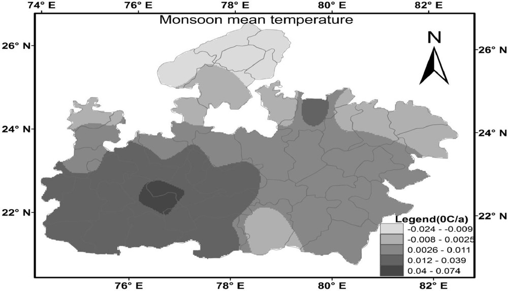
Spatial distributions of temporal change in monsoon mean temperature at Madhya Pradesh from 1901 to 2002.
Distribution spatiale du changement temporel dans la température moyenne de mousson à Madhya Pradesh, sur la période 1901 à 2002.
3.7.1 Maximum temperature trend
Fig. 7 showed the spatial distribution pattern of temporal change in the annual maximum temperature. The increase in magnitude of the annual maximum temperature varied from 0.0001 to 0.007 °C/year in most part of MP but it exceeded 0.007 °C/year in some areas, such as Seoni and Chindwara. The presence of bump near the border may be due to the interpolation that has been performed using observations inside the Madhya Pradesh. Fig. 8 shows the spatial distribution of winter maximum temperature whose magnitude varied from 0.0002 to 0.005 °C/year in most part of MP but it exceeded 0.005 °C/year in some areas, such as Balaghat station. Again the presence of bump near the border may be due to the interpolation that has been performed using observations inside the Madhya Pradesh. Furthermore, the magnitude of the summer maximum temperature (Fig. 9) varied from 0.007 to 0.03 °C/year from east to west MP. Fig. 10 shows the spatial distribution of monsoon maximum temperature. Some parts of MP show the cooling trend and some part shows the warming trend. The cooling trend has been observed in southwestern MP, which varied from −0.02 to −0.0001 °C/year and the remaining part of MP showed the warming trend, which varied from 0 to 0.02 °C/year. Therefore, it can be concluded that the annual, summer and winter maximum temperatures showed the warming trend over the entire MP and the monsoon maximum temperature showed the both increasing and decreasing trends.
3.7.2 Minimum temperature
The spatial distribution pattern of temporal change in the annual minimum temperature was shown in Fig. 11. The increase in magnitude of annual minimum temperature varied from 0.0001 to 0.0005 °C/year. The minimum increase was found in north MP and the maximum increase in west MP. Fig. 12 shows the increase in magnitude of winter minimum temperature, which varied from 0.0008 to 0.0014 °C/year from south to north MP. The summer minimum temperature (Fig. 13) magnitude was also increased; it varied from 0.001 to 0.03 °C/year from east to west MP. Unlike other seasons, monsoon season presented a positive and a negative trend, which can be seen in Fig. 14. The south and central MP showed the warming trend (0.002 to 0.017 °C/year); however, the northern edge of MP showed the cooling trend (−0.022 to −0.009 °C/year) from 1901 to 2002.
3.7.3 Mean temperature
Fig. 15 shows the spatial distribution pattern of temporal changes in the annual mean temperature. Similar to minimum and maximum temperature, the increase in magnitude has been observed in annual mean temperature over entire MP. The magnitude of annual mean temperature varied from 0.0001 to 0.0070 °C/year in almost all over the MP but drastically higher (0.02 to 0.08 °C/year) in some part of the Chhatarpur, Panna and Dhindhol stations. The winter season (Fig. 16) also shows the increasing trend, which varied from 0.001 to 0.01 °C/year over the MP, but it exceeded 0.01 °C/year in some part of Rewa district. In summer season (Fig. 17) also, the increase in magnitude was observed which varied from 0.008 to 0.03 °C/year from east to west MP. During the monsoon season (Fig. 18), the spatial distribution of mean temperature can be characterized by a decline from west-south MP to northeast MP. The increase in magnitude varied from 0.0025 to 0.07 °C/year in west and central part of MP. However, the decrease in magnitude varied from −0.024 to −0.008 °C/year in North, Northeast and some part of South MP.
3.8 Effect of urbanization on temperature
The degree of urbanization may be statistically inferred from several properties such as land cover, land use change, construction activities, automobile registration, and energy consumption. But individual effects of each statistic cannot be added to make a single meaningful quantity, i.e., the urbanization effect (Chung et al., 2004). Further, it is not possible to get the data of these parameters over a longer period. Population implies most of the activities related to urbanization. Therefore, in the present study population has been used as an index of urbanization to study the effect of urbanization on temperature. Table 4 shows the population and temperature during the LUP and MUP. The table further showed that the maximum, minimum and mean temperature is high during MUP than during LUP, indicating rise in temperatures with increase in urbanization. During LUP the maximum temperature decreases by 0.04 °C, but there is an increase of 0.32 °C during MUP, while the population was multiplied by 2.6 from LUP to MUP. Similar pattern has been observed in minimum and maximum temperature in MUP. Further, the minimum temperature is increased at higher rate (0.42 °C) followed by mean temperature (0.36 °C) and maximum temperature (0.32 °C) during the MUP. These findings are in conformity to the results of studies conducted by Wilbanks and Kates (1999) and DeGaetano and Allen (2002) wherein they reported the urban effect is more pronounced for minimum temperatures than maximum temperature.
Population et température pendant les périodes de moindre urbanisation et d’urbanisation plus prononcée.
| P | Population | Tmax (rate of change) | Tmin (rate of change) | Tmean (rate of change) |
| LUP | 15,542,150 | 31.97 (−0.04) | 18.75 (−0.03) | 24.79 (−0.03) |
| MUP | 40,063,461 | 32.30 (0.32) | 19.07 (0.42) | 25.11 (0.36) |
3.9 The relationship of air temperature and cloud cover
Cloud cover affects the temperature due to effect of cloud in reflecting and absorbing incoming visible solar radiation and outgoing infrared radiation. The effect of cloud on temperature depends on the balance of two competing effects; the cooling due to reduced solar radiation and the warming due to reduced outgoing long wave radiation. Table 5 shows the correlation coefficients between temperature variables (the mean, the maximum and the minimum temperatures) and cloud cover on annual and seasonal basis. It can be seen that total cloud cover is negatively related with temperature variables in annual and monsoon basis. However, a positive relation is found in winter and summer season. The annual maximum temperature shows the maximum significant negative correlation with cloud cover (−0.30) followed by mean temperature (−0.26). In monsoon season, strong negative correlation is depicted between cloud cover and mean temperature (−0.42) followed by the maximum (−0.41) and the minimum temperature (−0.40). Further, in summer season, only minimum temperature (0.26) showed the significant positive correlation with cloud cover.
Coefficients de corrélation entre couverture nuageuse et domaines de températures maximum, minimum et moyenne sur la période 1901 à 2002.
| Variables | Annual | Winter | Summer | Monsoon |
| T max | −0.30a | 0.10 | 0.12 | −0.41a |
| T min | −0.19 | 0.12 | 0.26a | −0.40a |
| T mean | −0.26a | 0.12 | 0.19 | −0.42a |
a Denote correlation that is significant at 5% significance level using the Kendall-tau method.
4 Discussion
The present study deals with an examination of variability and trends in annual and seasonal temperature variables (maximum, minimum and mean temperatures) for the 45 stations of MP, in central India. It was found that there are significant increases of 0.62 °C/102 years in the annual minimum temperature, 0.60 °C/102 years in the annual maximum temperature and 0.60 °C/100 years in the annual mean temperature over MP. These findings are in conformity to the results of studies conducted by Karl et al. (1993), Qiang et al. (2004) and Wibig and Glowicki (2002) which have shown that minimum temperatures have increased much more rapidly than the maximum temperatures. Henderson-Sellers (1995) reported that the causes of differential increase in the maximum and the minimum temperatures are closely related to change in cloudiness. Seasonal analysis showed that magnitudes of the positive trends in winter, summer and monsoon mean temperature were 1.20, 0.59 and 0.07 °C, respectively. The same pattern has been observed in maximum and minimum temperatures but the night temperature is found to be increasing more rapidly than day temperature. These results are following the same trend as over India (Arora et al., 2005; Kothawale and Rupa Kumar, 2005; Pant and Kumar, 1997). Pant and Kumar (1997) reported a significant warming trend of 0.57 °C per hundred years. Arora et al. (2005) also reported a significant increasing trend over India during the years 1940 to 2000 at the rate of 0.42, 0.92 and 0.09 °C/100 years in annual mean temperature, mean maximum temperature and mean minimum temperature, respectively. Further, present study findings are also consistent with the results of Kothawale and Rupa Kumar (2005), wherein they reported the significantly increase by 0.5 °C in annual mean temperature over India during the period of 1901 to 2003. Analysis on monthly time step indicates the significant warming trend in the months of February, March, April, October, November and December in the mean, the minimum and the maximum temperatures during the analysis period of 1901 to 2002. The increase in temperature during reproductive, grain formation and ripening phase of crops (February to March) is understood to be detrimental to productivity of wheat and other Rabi season crops due to terminal stress. The decadal variation of annual temperature variables shows that the temperature anomaly was positive after the 1951 to 1960 decade. The winter season mean temperature for sowing of Rabi crops in October to November was increased which can be detrimental for seed germination. Similarly for Rabi crops in reproductive phase (March to April) it may cause hastening in the maturity, reduce grain setting and grain number, and thereby reduce yield. Crops like wheat and chickpea suffer from higher temperature, particularly during grain filling. Soybean is the main crop grown on 77% of all agricultural land in MP. Lal et al. (1999) reported that if the maximum and minimum temperatures go up by 1 °C and 1.5 °C respectively, the gain in yield comes down to 35%. Further, they also reported that if maximum and minimum temperatures rise by 3 °C and 3.5 °C respectively, then soybean yields will decrease by 5% compared to 1998. This may ultimately affect the food security and economy of state and country.
5 Conclusions
The conclusions drawn from the study are as follows:
- • the significant increase in annual temperature is 0.62 °C (102 years)−1 in the minimum temperature, 0.60 °C (102 years)−1 in the maximum temperature and 0.60 °C (102 years)−1 in the mean temperature over MP;
- • seasonally, increase in magnitudes is 1.20, 0.59 and 0.07 °C in winter, summer and monsoon mean temperature, respectively. The same pattern has been observed in maximum and minimum temperatures but the night temperature is found to be increasing more rapidly than day temperature;
- • decadal variation of annual temperature shows that the warming trends have begun from 1961 onward;
- • analysis on monthly time step indicates the significant warming trend in the months of February, March, April, October, November and December in the mean, the minimum and the maximum temperature during the analysis period of 1901 to 2002;
- • the minimum temperature is increased at higher rate (0.42 °C) followed by the mean (0.36 °C) and the maximum temperature (0.32 °C) during the MUP with increased in population by around 2.6 fold from LUP to MUP;
- • further, cloud cover is significantly negatively related with temperature variables in monsoon season and as a whole of the year. However, in summer season, positive correlation is found between cloud cover and temperature variables.
Acknowledgements
The authors are thankful to the Department of Science and Technology (DST), New Delhi for providing financial support during the study period. We are also thankful to anonymous reviewers for their thoughtful suggestions to improve this manuscript significantly.
Appendix
Detrended Fluctuation Analysis (DFA) method
DFA used in various time series (Chen et al., 2002; Maraun et al., 2004; Peng et al., 1994; Varotsos, 2005a, b; Varotsos and Cracknell, 2004; Weber and Talkner, 2001) to detect possible long-range correlations consist of the following steps:
1. The first step is to integrate the given time series x(i) of length N and construct the new time series using the equation below:
| (1) |
The integration exaggerates the non-stationarity of the original data, reduces the noise level, and generates a time series corresponding to the construction of a random walk that has the values of the original time series as increments. The new time series, however, still preserves information about the variability of the original time series (Kantelhardt et al., 2002; Varotsos and Kirk-Davidoff, 2006).
2. Next step is to divide the time series y(i) into ‘m’ non-overlapping segments of equal length d. For DFAn, in each segment ‘m’ a best fit polynomial trend pnd,m of order n is subtracted from the integrated y(i) time series:
| (2) |
When linear polynomials are used, the fluctuation analysis is called DFA1, for quadratic polynomials DFA2, for cubic polynomials DFA3, etc. By definition, DFA2 removes quadratic trends in the profile Y(i) and thus linear trends in the original series xi.
3. Calculate the fluctuation function F(s) for each segment m:
| (3) |
4. Then estimate the mean-squared fluctuation function by averaging over all segments:
| (4) |
5. Repeat this procedure for several d to get a range of fluctuations function.
Plot log F(di) versus log di, for i = 1,.,..,.m. If there is an obvious linear relationship between them, the least squares fitted slope provides an estimate of the scaling exponent α. An exponent (slope of log-log plot) α ≠ 0.5 in a certain range of N values implies the existence of long-range correlations in that time interval, while α = 0.5 corresponds to the classical random noise (uncorrelated data). If 0 < α < 0.5, power-law anti-correlations are present (anti-persistence). When 0.5 < α < 1.0, then persistent long-range power-law correlations prevail (anti-persistence) and when α = 1, it corresponds to the so-called 1/f noise. α > 1 implies that the long-range correlations are stronger than in the previous case with α = 1.5 corresponding to Brownian motion (Ausloos and Ivanova, 2001; Talkner and Weber, 2000).
Autocorrelation test of independence
The first order autocorrelation coefficient is especially important because for physically systems dependence on past values is likely to be strongest for the most recent past. This test is based on values of the correlation coefficients calculated from all pairs of data points separated by k time periods, where k, the lag time. Such autocorrelation coefficients between consecutive values of the same variable are called autocorrelation coefficients. The lag 1 serial correlation coefficient (Wallis and O’Connell, 1972) of annual temperature series was estimated using the Eq. (5) given below at 5% significance level for two-tailed test.
| (5) |
The first order autocorrelation coefficient r1, can be tested against the null hypothesis using Anderson (1941) limit for the two tailed test.
If the r1 value falls within the confidence interval given above, the data are assumed to be serially independent otherwise the sample data are considered to be significant serially correlated.
Mann–Kendall test
The MK test, also called Kendall's tau test due to Mann (1945) and Kendall (1975), is the rank-based nonparametric test for assessing the significance of a trend, and has been widely used in hydrological trend detection studies. It is based on the test statics S defined as:
| (6) |
A very high positive value of S is an indicator of an increasing trend, and a very low negative value indicates a decreasing trend.
| (7) |
It has been documented that when n ≥ 10, the statistic S is approximately normally distributed with the mean
| (8) |
| (9) |
The standardized test statistic Z is computed by as follows:
| (10) |
The null hypothesis, H0, meaning that no significant trend is present, is accepted if the test statistic Z is not statistically significant, i.e. −Zα/2 < Z < Zα/2, where Zα/2 is the standard normal deviate.
Theil–Sen's estimator
The slope of n pairs of data points was estimated using the Theil–Sen's estimator (Theil, 1950 and Sen, 1968) that is given by the following relation:
| (11) |
In which 1 < j < i < n and β is the robust estimate of the trend magnitude. A positive value of β indicates an ‘upward trend’, while a negative value of β indicates a ‘downward trend’.
Trend-free pre-whitening
The TFPW-MK procedure of Yue et al. (2002) is applied in the following manner to detect a significant trend in a serially correlated time series.
1. The slope (β) of a trend in sample data is estimated using the approach proposed by Theil (1950) and Sen (1968). The original sample data Xt were unitized by dividing each of their values with the sample mean E(Xt) prior to conducting the trend analysis (Yue et al., 2002). By this treatment, the mean of each data set is equal to one and the properties of the original sample data remain unchanged. If the slope is almost equal to zero, then it is not necessary to continue to conduct trend analysis. If it differs from zero, then it is assumed to be linear, and the sample data are detrended by:
| (12) |
2. The lag-1 serial correlation coefficient (r1) of the detrended series Xt is computed using Eq. (5). If r1 is not significantly different from zero, the sample data are considered to be serially independent and the MK test is directly applied to the original sample data. Otherwise, it is considered to be serially correlated and AR (1) is removed from the X′t by
| (13) |
This pre-whitening procedure after detrending the series is referred to as the trend-free pre-whitening (TFPW) procedure. The residual series after applying the TFPW procedure should be an independent series.
3. The identified trend (Tt) and the residual Y′t are combined as:
| (14) |
The blended series (Yt) just includes a trend and a noise and is no longer influenced by serial correlation. Then, the MK test is applied to the blended series to assess the significance of the trend.


