

1 Introduction
It has recently been shown that correlations of ambient seismic noise can be used to retrieve the elastic response of the Earth between two receivers (Shapiro and Campillo, 2004). This property has consequently become a widely used tool in seismic imaging efforts (Lin and Ritzwoller, 2011; Shapiro et al., 2005). The inherent temporal stability of noise correlation measurements (e.g., Stehly et al., 2006) has subsequently led to time-dependent analyses to detect elastic parameter variations in the Earth's, crust, and has successfully been implemented in various contexts and media (Brenguier et al., 2008a,b; Clarke et al., 2011; Diane et al., 2011; Wegler and Sens-Schoenfelder., 2007; Mainsant et al., 2012; Renalier et al., 2010). To optimize the sensitivity of these measurements, it is convenient to analyze the temporal changes of the coda of the correlations rather than those of the direct waves (Poupinet et al., 1984; Snieder et al., 2002). It is important to note that the coda of the correlation function exhibits some properties that are characteristic of the actual recorded coda. Indeed, Sens-Schoenfelder and Wegler (2006) showed that the envelope of the latter part of the correlations presents a decay similar to that of the actual coda. Using correlations of the coda of correlations (C3), Stehly et al. (2008) further showed that the latter consists of multiply-scattered arrivals. This C3 function actually converges towards the Green's function, as does the coda of actual seismograms (Campillo and Paul, 2003). This argument provides a firm basis for the use of the coda of correlations in monitoring efforts, given that the late part of the correlation contains multiply-scattered physical arrivals, just as the early part contains the direct waves. That being said, the degree of accuracy or robustness required in the reconstructed phases of the correlation varies as a function of the application. In the case of standard surface wave tomography, where strong lateral variations are expected and where a posteriori uncertainties on the models are significant, direct wave velocity uncertainties of less than 1% are generally acceptable. For monitoring, the temporal variations of relative velocities that are observed are far smaller than this value. For example, the typical variations prior to volcanic eruptions were measured to be at most of the order of 0.1% (e.g., Brenguier et al., 2008b), and post-seismic responses of the same order have also been detected (e.g., Brenguier et al., 2008a; Chen et al., 2010). Such large fluctuations of seismic velocities are unambiguously related to seismic or volcanic events, both in terms of causality (Brenguier et al., 2008a) and spatial location (Obermann et al., 2014). In a recent study of the continuous records of the Hi-Net network in Japan, Brenguier et al. (2014) observed fluctuations of the seismic velocity of the order of 10−4 in the absence of large tectonic disturbances, but without specific corrections for external forcing effects. There are therefore clear observations that confirm the feasibility of ambient noise monitoring.
The practical application of temporal monitoring to the forecasting of events such as volcanic eruptions requires a complete understanding of the origin of observed velocity changes, including the weak ones. Such fluctuations have various sources, and can be associated with instrumental issues (e.g., Stehly et al., 2007), with external forcing such as precipitations (Hillers et al., 2014; Nakata and Snieder, 2012; Sens-Schoenfelder and Wegler, 2006), regional water load (Froment et al., 2013), tides (Hillers et al., 2014; Takano et al., 2014; Yamamura et al., 2003), or thermoelasticity (Hillers et al., 2014). Given that these fluctuations are correlated with external parameters that are commonly recorded and have seasonal components, there is a prospect that they can be detected and eventually accounted for.
A more difficult issue is the sensitivity of the cross-correlation to spatial-temporal variations in the noise source. The theoretical requirement for a perfect reconstruction of the Green's function includes the azimuthal isotropy of the field incident on the receivers (a complete discussion is beyond the scope of this paper and we refer here to Campillo and Roux (2014) and the references herein). When the spatial distribution of the incident field is non-isotropic, a possible bias in the arrival times extracted from the cross-correlations has to be considered. For example, Tsai (2009), van der Neut and Bakulin (2009) and Yao and Van Der Hilst (2009) discussed the travel time bias produced in noise-based measurement by a non-isotropic distribution of noise intensity. Although Hadziioannou et al. (2009) showed that an imperfect reconstruction by itself does not impair the detection of wave velocity changes, we discuss here the problem of a time-varying anisotropic noise intensity distribution.
The effect of source anisotropy on correlation functions is a subject of long-standing interest, with the earliest forays dating back almost 40 years, see Cox (1973). Weaver et al. (2009) has since argued that the anisotropy of a smooth azimuthal distribution of noise intensity does not impair the accurate reconstruction of direct wave arrival times when the receivers are separated by a distance that is much larger than the wavelength. For more realistic configurations when the distance is finite, Weaver et al. (2009) gave approximate analytical results for the travel-time bias produced by the anisotropic character of the azimuthal distribution of the noise field. Froment et al. (2010) verified this theory with real data to demonstrate that these effects can be quantified and eventually corrected. Their conclusion was that the biases expected from a smooth distribution of intensity are predictable and small, in most cases, when considered in the context of seismic tomography. We note here that the smoothness of the azimuthal distribution of noise intensity is largely guaranteed by the presence of scattering at frequencies higher than 0.1 Hz. The importance of scattering was illustrated by Froment et al. (2010), who considered a very unfavorable incident field distribution to show that the bias is reduced when coda waves are correlated as opposed to direct arrivals. This is naturally expected given the role of scattering in azimuthally homogenizing the wavefield (Campillo, 2006). However, selecting scattered waves is impossible when using ambient noise records given the continuous nature of the source, which may result in biased arrival times for the direct waves extracted from the correlation. Since the noise source (mostly oceanic gravity waves) is evolving with time, we should be mindful of non-physical apparent velocity variations solely due to the changes in the azimuthal distribution of intensity. It should furthermore be noted that we are not referring to possible changes in spectral content that are easy to mitigate. In this paper we aim to test the stability of the correlation function and to evaluate the robustness of relative velocity change measurements made in coda windows when the noise source is highly anisotropic. We perform numerical simulations in a medium with significant scattering in the chosen frequency band, and further demonstrate similar effects using real data recorded on a volcano in multiple-scattering conditions.
2 Numerical simulation of coda signals in a scattering unbounded 2D medium
2.1 Simulations set-up
We extend the work of Colombi et al. (2014) who simulated flexural waves on a 2D plate to investigate the role of reverberations and source distribution on the quality of the cross-correlation reconstruction. We now simulate wave propagation in a 2.5 m × 2.5 m × 2 mm thick plate that contains a circular region (radius 0.6 m), where 220 scatterers are randomly distributed (Fig. 1a), thus generating multiple scattering. The material properties of the homogeneous plate are those of aluminium, characterised by Vp = 6100 m/s, Vs = 2900 m/s and ρ = 2700 kg/m3. The scatterers are either fast or slow circular inclusions with diameters varying between 2 and 3 cm. The P and S velocities are either halved for slower inclusions or 50% faster for fast inclusions, while ρ is set at 2000 kg/m3. A pair of receivers 0.5 m apart is centered in the scatterer's region. Both are kept sufficiently distant from the inclusions to avoid near-field effects (e.g. resonance inside the scatterers). A spectral element approach was chosen for this numerical analysis. Plate motions are simulated using the SPECFEM3D software (Peter et al., 2011), and the discretization of the plate and scatterers is straightforward with the CUBIT software package. We model the boundary of the scatterers explicitly, which results in an adaptive paving scheme for the meshing. The smallest element edge (down to 2 mm) drives the cost of the simulation by defining the size of the integration time step according to the stability condition. By using the source–receiver reciprocity as in Colombi et al. (2014), only two forward simulations are required (using each receiver as a source) to calculate the wavefield. The computational cost is therefore limited.
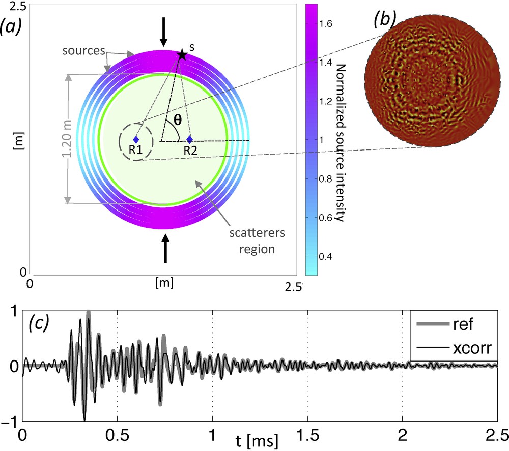
(Color online) (a) The source–receiver layout on the plate reproduced in the simulations. The four rings of sources (∼200), forming an annular region, are placed just outside the area containing scatterers and receivers (bound by the light green circle). The angle 0 ≤ θ ≤ 180∘ is taken in a counter-clockwise fashion. The four boundaries are modeled with the PML condition to suppress reflections. When source anisotropy is included, the intensity is distributed according to the colormap (for B2 = 0.6). This is equivalent to a noise directivity indicated by the black arrows. (b) One snapshot of the propagation in the scatterering region with the source located at R1. (c) Comparison between the reference signal (thick grey line) and the causal part of the stacked cross-correlation (black line) computed using a uniform intensity distribution. Amplitudes are normalised.
Perfectly matched layer (PML) conditions are applied to the left and right lateral boundaries while the top and bottom sides are modelled as free surfaces. Such requirements render this type of study difficult to implement in a laboratory setting, unless dynamic environments such as those in Vasmel et al. (2013) are employed.
Roughly 200 receivers (set up as sources, given reciprocity) are distributed among four rings surrounding the scattering region (Fig. 1a). By choosing such an annular surface of sources instead of a simple circular distribution, we minimize the non-physical contributions highlighted in previous studies (e.g., Colombi et al., 2014). The sources consist of vertical point forces with a Ricker wavelet centered at 35 kHz acting perpendicularly to the plate's surface, resulting in mainly A0 Lamb waves in the plate (Colombi et al., 2014; Larose et al., 2007). For this reason, only the vertical component of the displacement is used in the cross-correlation. The computational domain is assumed to be non-dissipative and elastically linear. Signals are sampled at 500 kHz, and a band-pass filter between 15 kHz and 45 kHz is applied to the signal in order to eliminate numerical noise. Lamb wave dispersion in the 15 kHz to 45 kHz frequency band yields wavelengths ranging from 1.5 cm to 5 cm. With a phase velocity of the A0 mode reaching c = 2000 m/s at 40 kHz, the direct wave (featuring a faster travel time) and the scattered coda are contained in a 2.5-ms-long signal (Fig. 1b). The displacement uz for the simulation is uniformly computed over the surface using a grid of 3-mm-spaced receivers in both x and y directions. This provides a full description of the wave propagation in the plate (e.g., Fig. 1b).
We compute the cross-correlation function for each individual source at the two receivers R1 and R2 (as represented in Fig. 1a) and we stack the results. The causal part of the stacked cross-correlation is shown in Fig. 1c. The reference “band-limited Green function” is the true Green function obtained by a single vertical force at one of the receivers. The two traces are nearly identical, even in their late part. Here, the individual correlations have been normalized by their energies to simulate an isotropic noise source distribution and therefore to optimize the quality of the reconstruction.
2.2 Beam forming and scattering mean free path in the plate
We first investigate the nature of the scattered wavefield via beam forming (hereafter abbreviated as BF). This technique provides directional and velocity information about the elastic energy propagating in the plate by mapping records from a 2D array of receivers to a 2D plane wave domain (Boué et al., 2013; Rost and Thomas, 2002). BF is used here to analyze the field content in different windows corresponding to direct and coda waves. Fig. 2a depicts BF results obtained for an “antenna” with an aperture of 30 cm, containing 200 receivers and a single source. The center of the antenna corresponds to the receiver R1 in Fig. 1a. The ideal approach discussed in (Boué et al., 2013) has been followed, and we compute the BF for a 0.3 -ms- long moving window. Fig. 2b depicts the strong directivity of the incident field when the window is centered on the first arrival. First-order effects of scattering are already visible with a clear spread of incident intensity away from the direct path. Nevertheless, the field comes prevalently from the right side. The weak spot to the left is attributed to the small imperfection of the PML boundary layer in the simulation. The BF is then applied to a coda window, resulting in the field illustrated in Fig. 1c. In this case, the intensity distribution presents a wide azimuth (Fig. 2c), and it is difficult to recognize a dominant direction associated with the source. The characteristics of the two regimes illustrated in Fig. 2 b and c are used in the interpretation of the effects of noise anisotropy.
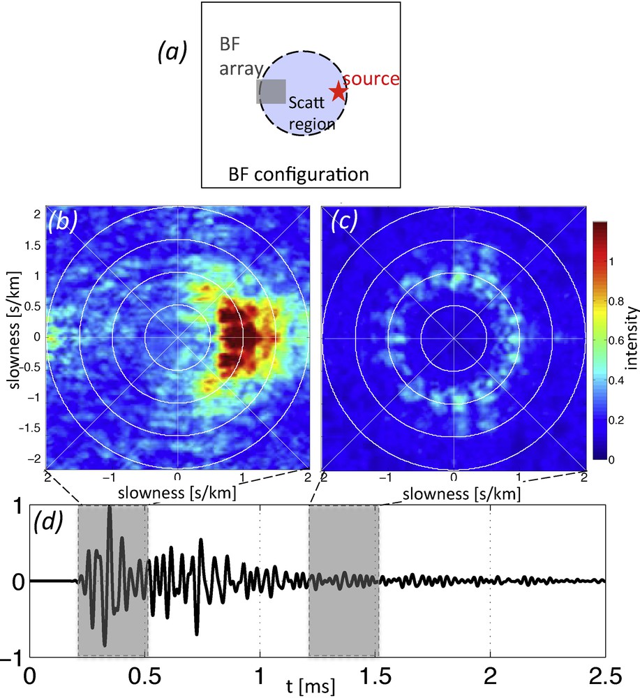
(Color online). (a) The layout used for the beamforming analysis. The antenna is 30 × 30 cm large with ∼200 receivers. The source is located near the edge of the scattering region, 50 cm away from the center of the array. (b–c) Snapshots of the BF corresponding to the time windows indicated in (d).
For scattering problems, a key parameter is the scattering mean free path l, or conversely the scattering mean free time tl = l/c (e.g., Sato, 1978). From the work of De Rosny and Roux (2001), l is derived from the exponential distance dependence of the ratio of coherent to incoherent intensities. The coherent intensity is obtained by calculating the intensity of the average seismogram for a given traceable arrival (in this case, the direct wave). The average here is performed on seismograms corresponding to the same source–receiver distance. On the other hand, the incoherent intensity corresponds to the average of the intensities computed for each seismogram. The estimation of l is finally obtained through a linear regression of the logarithm of the intensity ratio as a function of the distance from the source (De Rosny and Roux, 2001) see Eq.(3). Here, we consider recordings from a 2D array for a source situated in the middle of a scattering region. In the frequency band considered, the value l of the A0 mode varies between 0.4 and 0.7 m, hence of the order of the distance between receivers (0.5 m).
3 Coda stability vs. noise distribution anisotropy
(Froment et al., 2010) have considered azimuthal intensity distributions B(θ) of the following type to study the sensitivity of the direct arrival reconstructed via cross-correlation with respect to the anisotropy of the noise distribution:
| (1) |
Here θ is the source azimuth measured as indicated in Fig. 1a, B0, B1 . . . are coefficients with values between 0 and 1. An isotropic source distribution will result from taking B(θ) = B0. Note that only cosine distributions are considered. This azimuthal parity flows from the fact that correlations between two receivers do not distinguish between arrivals with incidence θ or −θ in a locally homogeneous medium. The fact that only the even part of any arbitrary distribution of intensity has to be considered does not represent a limitation to the generality of this analysis. Froment et al. (2010) analyse whether and when the influence of large-scale heterogeneities across the source region should be taken into account in the calculation of the travel-time bias due to source anisotropy. The case where B(θ) = B0 + B2 cos 2θ with B0 = 1 and B2 = −0.6 represents a rather extreme case of anisotropy for the frequency range considered in our applications in which scattering is always significant. At larger periods, and if scattering is negligible, the noise may consist of very directive arrivals, in the form of isolated plane waves for example, challenging the necessary conditions to consider noise correlations as representative of the Earth response. In the present study, and in the context of noise based monitoring, we consider the case with B0 = 1 and B2 = −0.6 to illustrate the effect of a drastic change in the intensity distribution with respect to the isotropic scenario. Fig. 1a represents the corresponding source intensity of the synthetic ‘noise’, depicted by a color scale superimposed on the source locations. The arrow shows the dominant direction of the energy, being in this case perpendicular to the receiver pair strike and to the end-fire lobes (Roux et al., 2005).
For receiver distances larger than the wavelength, the travel time error δt of the direct wave for the anisotropic noise case can be calculated for positive correlation times following Weaver et al. (2009):
| (2) |
Given that the Green's function between two stations is rarely available for real media, monitoring studies are based on variations with respect to a reference cross-correlation stack. In the present case, we construct the reference cross-correlation function from an isotropic intensity distribution B(θ) = B0. To further simulate correlations of anisotropic noise fields, the cross-correlation for each individual source is modulated according to B(θ) (Fig. 1a) before stacking. The analysis is limited to the causal part of the correlation. Given the reference and the perturbed signals, the lag times are calculated using the doublet (or multiple window cross spectral) method of Poupinet et al. (1984).
Froment et al. (2010) used real data records and considered in detail the case where only the coherent part of the intensity (i.e. that obtained by muting the signal after the ballistic wave) is used. The same process has been performed here with synthetic data using only the first arrival (between 0 and 0.5 ms according to Fig. 1c). When incident field anisotropy is present, we measure values of δt that are similar to their study and well predicted by Eq. (2).
We then compute the cross-correlation using the full 2.5-ms signals that include both direct and coda waves. A moving window of 0.3 ms has been used here to calculate the lag-time δt. The windows partially overlap and the value of δt, obtained via the doublet method (dots in Fig. 3a) are plotted for the center of the moving window. The correlations for the isotropic case (B(θ) = B0) and anisotropic case (B2 = 0.6) are plotted in Fig. 3b, and a time lag bias is clearly visible on the direct wave. In Fig. 3a we show the evolution of the bias along the time axis of the cross-correlation. The peak value of δt(τ) for the direct wave can be comparatively estimated by Eq. (2), (short green line in Fig. 3a, by setting ω0 = 2π · 35000 rad/s, and τ = 0.25 ms. We note that this theoretical prediction is not quite reached in the numerical experiment, most likely due to the effect of scattering, which generates a variety of incidence angles for each individual source (Figs. 2b and c). The scattering thus has a smoothing effect on the imposed anisotropy of the source azimuthal intensity.

(Color online) (a) The error δt(τ) is depicted by the blue dashed line while the fractional error δt(τ)/τ is in red for the traces shown in (b). The scale for δt(τ)/τ is in percent (right axis). Each dot represents the center of the window used to estimate δt. The green line represent the relative error predicted using Eq. 2 for the first arrival. (b) Comparison between the unperturbed cross-correlation and the perturbed one.
δt drops rapidly after the arrival of the direct wave, and then fluctuates at a level that does not seem to evolve in time and is on the order of one third of the direct wave bias. As is commonplace in monitoring studies, we define the fractional time delay as δt(τ)/τ. This quantity is the opposite of the fractional velocity variation for a homogeneous change in the medium, and is represented by the dashed blue line in Fig. 3. δt(τ)/τ calculations for arrivals following the direct wave converge to very small error values on the order of ≤10−4. It should be noted that the spectral coherency of the signal remains always above 90%, suggesting that the introduction of source azimuthal anisotropy does not provoke major changes in the structure of the complex coda waves reconstructed by correlation.
This numerical result indicates that correlation coda waves exhibit a weaker sensitivity to source anisotropy compared to direct waves. For monitoring applications, this means that correlation-based coda waves are expected to be weakly sensitive to changes in the ambient noise source distribution. We thus observe a rapid drop of the bias after the direct wave and a high coherency between isotropic and anisotropic scenarios. The relative delay δt(τ)/τ measured in the late coda of the synthetic correlations for a large change in source distribution is of the same order (10−4) as the actual fluctuations measured by Brenguier et al. (2014). In the following section, we perform a similar test with real data, where a database of small impulsive signals allows us to reproduce the synthetic setup fairly accurately.
4 Real data from Erebus volcano
We use a set of small impulsive icequakes to mimic the role of the vertical forces in the previous numerical experiment. A large database of such records is available from the broadband portion of a temporary network of seismometers deployed on the upper edifice of Erebus volcano, Antarctica (Knox, 2012; Zandomeneghi et al., 2013). Given the rapid decay of the direct waves for icequake peak frequencies of 1-3 Hz, we compute vertical component cross-correlation gathers for inter-station pairs with distances short enough for the Rayleigh wave to be both visible and distinct from other phases. Furthermore, given the extremely short scattering mean free path (several hundred meters to a few kilometers) computed for these frequencies on Erebus volcano (Chaput et al., in press), we only compute cross-correlations using events for which the direct ballistic arrivals show high signal-to-noise ratios. Naturally, if the event is too far from the station pair, the recorded envelope rapidly becomes emergent in character and the multiple scattering contribution to the correlation function will tend to dominate any de-phasing of the Rayleigh wave due to anisotropy in the illumination. We compute the correlations using a 7.5 s window encompassing the direct waves and a part of coda for all events within a maximum of 3 km of the closest station in the selected pair. Contributions from sources that lie within a circular region between the station pairs are removed to better match the numerical experiment. We first compute a reference using all events in this range, representing an isotropic illumination of the receivers, and then progressively limit the source distribution away from the inter-station strike by a factor of 2θ. For the reconstruction to be adequate, a sufficiently large number of sources must remain in the limited distribution to allow for coda convergence. Figure 4 shows an example of this for two stations (6 s of correlation shown) and an angular opening of θ = 70∘, clearly showing the de-phasing of the Rayleigh wave followed by an abrupt recovery in phase for the coda portion of the correlation. It should be noted that the corresponding δt(τ)/τ for the direct wave is on the order of a few percent, thus making this effect worthy of consideration if the direct wave is used to infer temporal change in the medium. δt values in the coda fluctuate on the order of one fourth of the direct wave bias. Despite unfavorable experimental conditions including source variability and locations in the vicinity of the receivers, we observe that the average δt(τ)/τ measured in the early coda (2 -6 s) is roughly 0.001, more than 30–50 times less than for direct waves. Here, we have presented a single station pair to reproduce the numerical results as closely as possible, and we are consequently dealing with issues arising from poor signal-to-noise ratios later in the coda. When many equidistant station pairs are available, averaging the δt(τ)/τ measurements over similarly spaced pairs will necessarily reduce coda fluctuations, and we can therefore expect far more accurate and smooth results. Furthermore, studies using ambient noise benefit from a nearly limitless quantity of data, whereas only limited sources are available in the present case. Therefore, the error estimate for the coda presented here should be considered a practical upper-bound scenario.
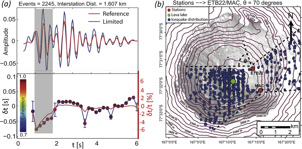
(Color online) a) Top panel, comparison of the vertical-vertical reference cross-correlation function with the cross-correlation function obtained from the limited distribution shown in b) (causal portion shown, pre-Rayleigh signal removed), at stations MAC and ETB22. a) Bottom panel, δt (black line), associated coherence values (colored dots), and δt/t (red line) for a 0.5 s window and an overlap of 0.2 s. Note that the de-phasing that occurs in the Rayleigh wave falls off very rapidly in the coda.
5 Discussion and physical interpretation
In the following, we discuss the sensitivity of coda waves to noise distribution anisotropy as derived from the basic properties of scattered waves. Firstly, we elaborate on the specific portions of the propagation paths that are sensitive to anisotropy of the noise source. Figure 5 presents a depiction of a scattered wave path. Let us consider the correlation of signal in A with signal in B, that is, the propagation from A to B.

(Color online) Sketch of one of the scattering paths produced by a wave front (thick arrow) generated by a distant noise source.
The direct path between A and B is sensitive to the anisotropy of the noise incoming around the direction θ = 0. The coda waves consist of the superposition of the contributions of various scattered paths, as the beam forming results in Fig. 2 illustrate. It is further useful to view a given multiply scattered path as a random walk process (e.g., Gusev and Abubakirov, 1987; Margerin et al., 2000). For such a random path, the bias produced by the anisotropy of the incident intensity distribution exclusively affects the part of the path between the receiver acting as a virtual source (here defined as A) and the first scatterer (S1, Fig. 5). The rest of the path (the black trace in Fig. 5) is not affected if we assume that the scatterers do not move. In the following, we neglect the effect of the initial anisotropy of the noise field on the intensity of the field produced by the first scattering event. The bias δt is therefore independent of the number of scattering events and of the total length of the path. We note that we observe this behavior in the numerical experiment and in the real data with fluctuations of the bias independent of the lapse time (Figs. 3 and 4). In practical applications of monitoring, the detection of a homogeneous velocity change assumes a constant fractional delay δt(τ)/τ. The bias due to anisotropy of the noise direction does not produce such a constant fractional delay.
We use Eq. 2, valid for the bias of the direct wave only, to evaluate the sensitivity of the path between the virtual source and the first scatterer. We call lf the distance A–S1 for this particular path in Fig. 5. The travel time between A and S1 is given by tf = lf/V. When using Eq. 2, the relative error produced by anisotropy for a single scattering path can be written as:
| (3) |
where θ is the azimuth of the path A–S1.
This result is however only valid for a single path, and a statistical generalization is required. The characteristic average distance between the source and the first scatterer is given by the scattering mean free path l, and the corresponding mean free time, tl = l/V. For our purpose, l can be considered as the distance for which, on average, the wave behaves as a direct wave. We know that the average travel time between scattering events t is given by tl, the mean free time, but the summed average timing error has to be computed in accordance with the underlying statistical distribution of the propagation time between two scattering events.
A discussion of the statistics of distance (or equivalently of time) between scattering events in the diffusion regime is outside the scope of this paper. We refer instead to Heiderich et al. (1994), who showed that diffusion in a medium with anisotropic scattering can be described by a random walk process when the step length follows an exponential distribution. In our case, this means that the statistical distribution of lf is of the form:
| (4) |
We recall that l represents the mean free path, while lf the distance between the receiver and the first scatterer for a particular configuration (Fig. 5). The average of δt cannot be computed directly because of the divergence of Eq. (2) when t approaches 0. Indeed, this limit is not in the validity range of the results of Weaver et al. (2009). To identify a realistic and conservative upper bound of the average value <δt>, we add the constraint that δt must be smaller than t. This leads to the upper bound <δt > max that we compare with the value of δt computed for t = tl through the ratio:
| (5) |
For the source distribution anisotropy depicted in Fig. 1a (B2 = −0.6), and choosing parameters characteristic of monitoring at the crustal scale (frequency∼1 Hz), we obtain R = 3.9 for tl = 30s and R = 2.9 for tl = 10 s. We now make use of the approximation and we apply the correction R.
We extend this analysis for a single path and a single azimuth to all the different paths that contribute to the coda by averaging the bias δt over the azimuth θ of the first scatterer. Coda waves consist of multiple arrivals following pseudo-random paths. Consequently, the analysis we propose for a single path must be generalized to an ensemble of paths, or, in other words, to a distribution of first scatterers such as S1′ on Fig. 5. We assume that these scatterers are evenly distributed, with an average distance to A of l. For each path, the coda of the correlation is affected by the anisotropy of the incident intensity by a bias δt. If we assume that the contributions of each path to the final result are equal and their time shifts δt are small (ω0δt < 1), the total contribution is subject to a delay <δt> that is simply:
| (6) |
Whereas the bias expected for direct waves is the maximum value of the term , we note that the coda could not suffer from such an elevated bias, since it is represented by the average value of the term that is governing the error associated with source distribution anisotropy. When considering the same extreme case of anisotropy as used in the numerical simulations in section 3, we note that the term has a max value of 6, leading to the theoretical error plotted in Fig. 3a (green line centered on the direct arrival). The average value , however, is 1. This contributes to the weaker sensitivity of coda waves and explains the rapid drop of <δt> when passing from direct to coda waves, noted in both numerical simulations and real data.
We have tested the relation (6) with two examples. It is important to recall here that the physical parameter that is monitored is the seismic velocity C, through its relative variation:
| (7) |
These agreements show that this simplified approach allows use to predict the expected level of error in monitoring studies. It is also worth noting that our expression yields an upper bound estimate, and we may therefore expect fluctuations smaller than 10−4 when using waves in the late coda. We further anticipate very good precision for the two end-members of scattering regimes observed in practice. For weak scattering, i.e. mean free path larger than inter-station distance, and measurements in the late coda, Eqs. 6 and 7 indicate that large tl and τm imply small fractional errors. Strong scattering, on the other hand, implies that the effect of scattering on the incoming source wavefield cannot be neglected. Given that the scattered wavefield rapidly converges to a smooth and isotropic intensity distribution, the expected falls naturally to 0 and a perfect reconstruction is expected for the correlation function (e.g., Colombi et al., 2014). An absence of bias even for direct waves is then expected, as is shown by Froment et al. (2010).
6 Conclusions
We demonstrate here that ambient noise monitoring is subject to very small errors in the presence of a temporally evolving source distribution if the coda of the correlation is used as a comparative metric. The measurements of fractional delay are far more stable for coda waves than for direct waves, due to the intrinsic properties of scattered waves. We propose a simplified approach to evaluate the sensitivity of correlation functions to noise anisotropy based on previous results obtained for direct waves. With this simple analysis, we are able to correctly estimate the errors produced by anisotropic source distributions in numerical experiments, and these effects are further documented for real data on Erebus volcano. This generalization also yields realistic values for the ambient monitoring precision observed at the crustal scale with real data. Furthermore, this analysis shows that high-precision noise-based monitoring could be performed with coda waves even in the presence of unknown azimuthal variations in the intensity distribution of the noise source. In practice, averaging over roughly equidistant stations pairs will further reduce the bias associated with the temporal evolution of the noise source distribution.
Acknowledgements
This work was supported by the European Research Council (Advanced grant Whisper L27507). GH enjoys support from the Heisenberg program of the German research Foundation (DFG). We thank K. Nishida and A. Rovelli for their constructive reviews. Associate Editor James Badro and Editor Vincent Courtillot thank Barbara Romanowicz for her evaluation of this paper. The computations were performed using the High-Performance Computing infrastructure CIMENT (https://ciment.ujf-grenoble.fr), which is supported by the Rhône-Alpes region (GRANT CPER07_13 CIRA: www.ci-ra.org), France Grilles (www.france-grilles.fr), and the CNRS MASTODONS program. The data used in this study are available through the IRIS Data Management Center. The facilities of the IRIS Consortium are supported by the National Science Foundation (USA) under Cooperative Agreement EAR-1063471, the NSF Office of Polar Programs and the DOE (USA) National Nuclear Security Administration.