

1 Introduction
Correlation between stratigraphic sections provides significant information about the chronology and geometry of sedimentary structures. However, significant uncertainty may exist in stratigraphic correlation, depending on the considered scale, the spacing between sections, the quality and type of observations, and the concepts used to analyze these observations. As observed by Doveton (1994) in the case of geophysical well-logging data, manual methods for well correlation can be slow, labor-intensive, expensive, and sometimes inconsistent owing to uncertainties. Moreover, several sets of correlations may match the same sparse observations while honoring a given set of interpretive rules (Borgomano et al., 2008; Koehrer et al., 2011). As shown by Bond et al. (2007) for seismic interpretation, cognitive bias may also be introduced, depending on the background of the interpreter. This means that the expert knowledge necessary in all interpretive processes may sometimes orient the interpretations in an inappropriate way. This can be a problem especially when this expert knowledge is not well documented.
In subsurface studies, errors in correlation between boreholes can be consequential. For instance, in stratigraphic hydrocarbon reservoir forecasting, well correlation is typically required to extrapolate layer geometry, which in turn provides a coordinate system to simulate petrophysical properties with geostatistical methods (Dubrule and Damsleth, 2001; Larue and Legarre, 2004; Mallet, 2004, 2014, Pyrcz and Deutsch, 2014). In this context, a wrong stratigraphic correlation model is likely to yield inaccurate predictions about the layering and the associated porosity and permeability fields in the reservoir.
The rationale for this work is that automatic correlation should be used in conjunction with manual methods. Indeed, automatic correlation provides a unique way to make correlation results more systematic than expert interpretations (automatic approaches produce by definition reproducible results, whereas interpretations may vary from one interpreter to another). Additionally, the very large number of possible correlations (see Appendix A) makes stochastic methods appropriate to sample correlation uncertainty. However, to reach the same level of quality as with expert correlation, an important challenge for automatic methods is to translate qualitative stratigraphic concepts used in manual interpretation into computerized, quantitative rules. When this translation is effective, a clear benefit is to formally state the concepts involved in the correlation.
In this paper, we use a numerical method to stochastically build stratigraphic correlations from a set of 1D stratigraphic sections (also referred to as “wells” in this paper for simplicity; we further assume that all sections are pre-processed to provide the true stratigraphic thickness and eliminate discontinuities and reversals related to faults, recumbent folds or horizontal wells). Our method builds on The Dynamic Time Warping (DTW) algorithm, which was first used in geosciences by Smith and Waterman (1980) to build lithostratigraphic correlations. DTW is computationally efficient, relatively simple to implement and allows for varying the correlation cost function. This explains its large adoption for correlating facies (Howell, 1983; Smith and Waterman, 1980; Waterman and Raymond, 1987) and geophysical signals (Fang et al., 1992; Hale, 2013; Herrera et al., 2014; Hladil et al., 2010; Lallier et al., 2012, 2013; Wheeler and Hale, 2014). However, most of the above methods do not account for the distance between wells and neglect sequence stratigraphic concepts, although these constitute a paradigm of choice for correlation, see for instance Ainsworth (2005) for siliciclastic settings and Borgomano et al. (2008) for carbonate environments. Therefore, in this paper, we consider well data that correspond to sequence stratigraphic intervals identified from depositional facies. The proposed method (Section 2) generates several possible correlations of stratigraphic sequences according to sedimentological rules that account for the spacing between wells. These rules are described and applied to Cretaceous outcrops of the southern Provence Basin (southeastern France) in Section 3.
2 Proposed approach for sequence stratigraphic correlation
2.1 Dynamic Time Warping
Let us review the DTW method before discussing its adaptation to address uncertainty management in stratigraphic correlation. For two wells W1 and W2 with respectively n and m stratigraphic markers, DTW represents the stratigraphic correlation between these two wells as a path in a 2D cost table D of size n × m (Fig. 1A and B). This table is built up with a series of points and transitions corresponding to the correlation of markers and intervals, respectively. The geological consistency of each possible correlation between markers and between units and each possible unconformity is evaluated independently thanks to the computation of a cost. These costs are stored in the table as follows:
- • a point at cell (i,j) corresponds to the correlation between the marker i of the first well W1 and the marker j of the second well W2 with a cost c(i,j);
- • an oblique transition corresponds to a correlation between two intervals (the interval {i;i–1} of W1 and the interval {j;j–1} of W2) with a cost noted ti,i–1j,j–1 in Eq. (1);
- • a vertical transition between cells (i,j) and (i–1,j) means that the interval {i;i–1} of W1 ends in an unconformity between units j;j - 1 and j + 1,j of W2. This unconformity is associated with a cost noted ti,i–1j,j. A horizontal transition corresponds to an unconformity with a cost ti,ij,j–1.
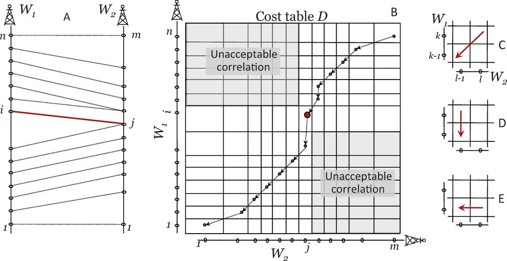
2D DTW for stratigraphic correlations. A: Stratigraphic correlation between two wells W1 and W2 containing respectively n and m markers. We assume the ith marker of W1 and the jth marker of W2 are known to be correlated (thick line). B: DTW cost table D displaying the minimum cost correlation path. Shaded parts are excluded to ensure the known correlation [i;j] is honored. The elements needed to perform stratigraphic correlation with DTW concern: the cost to conformably correlate units {k;k–1} of W1 and {l;l–1} of W2(C), the cost for unconformities to occur, i.e., for unit {k;k-1} of W1 to pinch out before crossing W2(D) and for unit {l;l–1} of W1 to pinch out before crossing W1(E).
The total score of a path is calculated as the sum of all the costs c and t contained in this path. The minimum cost path from the bottom left cell (bottom correlation line [1,1]) to the top right cell (top correlation line [n,m]) corresponds to the optimal correlation between W1 and W2. The minimum cost correlation path through the table is obtained by computing iteratively the minimum cost path from the bottom right cell to the cell (i,j) thanks to:
| (1) |
Once the entire DTW cost table has been filled, the correlation path is searched starting from the cell [n;m] as shown in Fig. 1. The next cell is the one with the minimum cumulated cost among the three adjacent cells (on the left, bottom and diagonally to the bottom left). The search then continues from this cell, using the same rule, until the bottom left is reached. This construction method makes the correlation path unidirectional, ensuring that no overlap occurs.
2.2 Framework to integrate the stratigraphic knowledge
In Eq. (1), conceptual correlation criteria can be integrated through the elementary cost c of correlating two given markers. For example, the costs detailed in Section 3.2 are based on a sedimentological analysis of carbonate facies that associates a range of paleo-bathymetry with each facies. From this information, it is possible to assess the consistency of the paleo-bathymetry for each possible correlation line using paleo-geographic criteria. We are currently investigating other types of elementary rules applicable in various stratigraphic contexts.
Unlike previous studies that assign a constant value to the correlation cost between stratigraphic units (term t in Eq. (1), see Smith and Waterman (1980); Fang et al. (1992)) or compute it as a function of the units’ thickness (Waterman and Raymond, 1987), our well correlation technique is based on the evaluation of depositional profile consistency (term c in Eq. (1)), which can typically have a sequence stratigraphic significance.
Nonetheless, our experience is that even the best rules can fail to produce a globally consistent correlation for long sections that display a strong variability of depositional conditions through time. Therefore, to increase the flexibility of the method and allow for diverse types of interpretive inputs, we propose to apply DTW so as to incorporate deterministic correlations and hierarchical information:
- • regional correlation surfaces can often be identified without ambiguity. Therefore, some correlation lines interpreted by a geologist can be taken as input constraint. For example, consider the deterministic input correlation line [i,j] in Fig. 1B. The correlation path is necessarily passing through this point in the DTW table and, by construction, almost half of the positions in the DTW table become unacceptable. As a result, the correlation problem can be divided in two so we directly build two DTW tables: one to compute the correlation path from [1,1] to [i,j], and another one to compute the correlation path from [i,j] to [n,m] (Fig. 1B);
- • stratigraphic sequences identified along wells can be ordered using a stratigraphic sequence hierarchy (Vail et al., 1977) or fractal considerations (Neal, 2009; Schlager, 2004, 2010). When such order information (sensu Vail et al. (1977)) is available, we apply DTW several times: lower-order stratigraphic markers are correlated, and the resulting correlation lines are used as input to the correlation of higher-order stratigraphic markers. In our current implementation, this strategy is only applied when the order for each marker is available.
In addition to providing interesting interpretive inputs, this simple strategy significantly improves the overall performance of the method by replacing a global DTW table by several much smaller tables.
2.3 Stochastic dynamic time warping
Classical methods to sample uncertainties about well correlations consist in randomizing the elementary correlation cost computation rules, leading to one single correlation per geological scenario (Griffiths and Bakke, 1990; Waterman and Raymond, 1987). As recently proposed for magnetostratigraphic dating (Lallier et al., 2013), the approach taken here is rather to generate several models for the same geological scenario. This approach essentially reflects the incompleteness of the input rules and could be combined in principle with cost randomization to explore scenario-based uncertainties. Each outcome of the method, associating all markers of all considered wells, is termed a realization because it samples correlation uncertainty.
To produce several realizations from a given set of costs, we use a stochastic transition when moving in the DTW cost table: from the current location (i,j) in the DTW cost table, the next location is randomly drawn by replacing Eq. (1) by:
| (2) |
| (3) |
2.4 DTW for multi-well correlation
The well correlation problem is generally not limited to a simple correlation between two wells but needs that d wells be considered, with d > 2. This could be addressed by using a d-dimensional DTW table (Brown, 1997). However, the time and memory complexity for d wells with n markers each is proportional to nd, making this method prohibitive for most datasets, even in optimized implementations (see Fuellen (1997) for a review). Wheeler and Hale (2014) propose an elegant and effective solution by casting the problem into a vertical shift optimization. However, their solution is deterministic.
Therefore, we simply correlate all wells two at a time by considering each pair independently. A correlation path is first built to define the pairs of wells that are to be correlated. This path should not contain loops to avoid inconsistencies (Fig. 2). This strategy is computationally efficient but does not guarantee that the resulting correlation is optimal. In particular, the well pair traversal order may be a source of bias when evaluating the cost functions based on depositional profiles (Section 3.2).

Example of inconsistent well correlation (thick line) generated using three pairwise correlations. This inconsistency is caused by the loop in the correlation path.
Therefore we have developed an iterative DTW (Fig. 3). First all pairs of wells connected by an edge of the correlation path are correlated. For a given edge e of the correlation path, all previously correlated pairs (from 1 to e–1) are known; if needed, they can be used to compute the current correlation. Once all wells have been traversed, an edge is randomly drawn and the corresponding pairwise correlation is rebuilt, taking into account all other correlations. This ensures that every correlation is generated knowing the whole 3D stratigraphic structure.
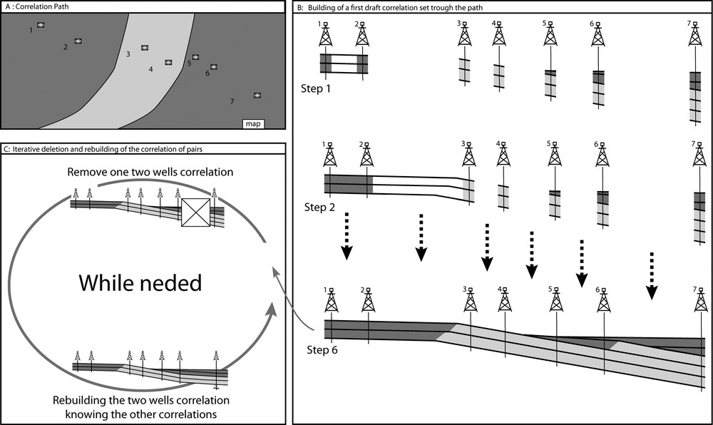
Iterative DTW algorithm. From a correlation path (A), a first correlation draft between wells is built (B) using a sequential 2D DTW. At each step of (B), the previously built correlations are known and used as a constraint. Then, to ensure the 3D consistency of the correlation, a random correlation between two wells is removed and rebuilt knowing all other correlations (C). This iterative process can be performed until the total score of the well correlation stabilizes.
This procedure may take a large number of iterations to converge to a stable, minimal cost correlation. However, we advise not to always iterate until convergence. Indeed, for uncertainty assessment purposes, the order by which the edges of the correlation path are traversed introduces an interesting source of variability, which is also probably present in manual expert-based correlations.
3 Application to outcrop data of the Beausset Basin
3.1 Geological settings and material
The Beausset basin is located in Basse-Provence, SE France (Fig. 4A). The studied area corresponds to a carbonate platform, aged Cenomanian–Middle Turonian and developed on the southern part of the “Durance swell” (Philip, 1974). These deposits display terrigenous inputs from a crystalline Hercynian basement corresponding to the southeastern limit of the basin (Fig. 4). Multiple outcrops have been described in this area (Gari, 2007; Philip, 1974, 1993; Philip and Gari, 2005) and almost continuous outcrop from platform to basin deposits allowed previous authors to build well-constrained geometrical models and sequence stratigraphic correlations.
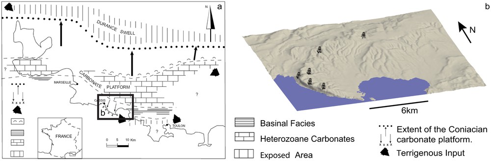
A: Geographic and paleogeographic settings of the study area. After Philip (1993). B: Location of the studied outcrops.
The studied outcrops are aged Lower Cenomanian to Middle Turonian (Fig. C.10). Nine outcrop sections covering the entire studied interval are used in this study (Fig. 4). The studied interval is subdivided in two primary stratigraphic units: U.I and U.II (Gari, 2007). U.I, aged Cenomanian, corresponds to the transgressive part of a second order, sensu Vail et al. (1991), transgressive regressive cycle ending mid Turonian (Philip, 1999). This unit is divided into six secondary stratigraphic units (U.I 1 to U.I 6), bounded by conspicuous surfaces or abrupt facies changes corresponding to third- and fourth-order cycles. The U.II primary stratigraphic unit, aged before mid-Turonian, is the regressive part of the second-order cycle started in U.I. This unit is also divided into six secondary stratigraphic units (U.II 1 to U.II 6). In this work, following the outcrop description and study proposed by Gari (2007), eight facies have been distinguished according to the depositional depth range, bioclastic content and deposition style (see Table C.1 Appendix C).
3.2 Stochastic well correlation
Correlation rules
Two methods for the evaluation of the consistency of a horizon are used: (i) a ramp paleo-angle-based rule that compares markers by pairs and (ii) a depositional facies based rule that uses all available markers of the considered horizon at once.
3.2.1 Paleoangle consistency
The slope of the paleo-depositional profile can be an important source of uncertainty in well correlation (Fig. 11). To check the consistency of a stratigraphic correlation of a carbonate ramp, Borgomano et al. (2008) introduce trigonometric relationships between average ramp paleo-angles (α and β) of two considered horizons and sediment thicknesses (e1 and e2 respectively on wells W1 and W2) according to (Fig. 5):
| (4) |

Trigonometric relationships on a carbonate ramp system (from Borgomano et al., 2008). Using measurement in A and relations B and C, the equality D is true if the correlation is good. pb: paleo-bathymetry at the current marker. sl: sea level. L: well spacing. bp: base profile. e1, e2: decompacted sediment thicknesses. α, β: angles between base profile and sea level.
This formalism is adapted to compute a cost of stratigraphic correlation between two markers b1 and b2 using a prior-defined correlation line (a1,a2) extracted for instance from seismic data or a reference surface. This reference line must be defined as input of the method and cannot be computed by the DTW method, which assumes that costs are independent of the path in the cost table. From the paleo-bathymetry at markers a priori correlated (pba1 and pba2), the paleo-bathymetry of the studied markers (pbb1 and pbb2) and the sediment thicknesses (e1 and e2), we compute the cost cA(b1,b2) as the degree of violation of Eq. (4) as:
| (5) |
This method is valid in the case of a regular accommodation increase between the two correlated wells. In the case of a differential subsidence, a rotation angle has to be added to Eq. (5) (Borgomano et al., 2008).
This correlation rule relies on a well log describing the bathymetry of deposition. As proposed by Leflon and Massonnat (2004), this bathymetry log curve is computed by Discrete Smooth Interpolation (Mallet, 2002) constrained by facies depositional depths (see Table C.1 in Appendix).
3.2.2 Sedimentary profile consistency
The boundaries of stratigraphic sequences identified on wells are often considered as time significant (Catuneanu et al., 1998). Consequently, markers bounding stratigraphic sequences could be taken as a sparse sampling of the geography (i.e. sedimentary profile) at the time of deposition. Evaluating the likelihood of a correlation line then boils down to checking whether this sampling is consistent with the paleogeography.
In this work, the cost for correlating two markers m1 of well W1 and m2 of well W2 is based on a zonation of carbonate facies with depth (membership functions, Fig. 7B) and on a regional theoretical bathymetric profile deemed representative of the paleogeography at the time of deposition (Fig. 7A). For our case study, the global analysis of the facies (Gari, 2007) led us to select a regional shelf slope of 0.5° to the south and to place the shelf break at a depth of about 40 m. For the slope below 40 m, we used an exponential north–south bathymetric profile for the carbonate ramp (Adams and Schlager, 2000):
| (6) |

Construction of depositional space. A. Bathymetric map built from the exponential equation (6). B. Membership functions for the description of the location of facies using bathymetry. C. Examples of possible location of deposition for facies 1, 3, 5, and 6.
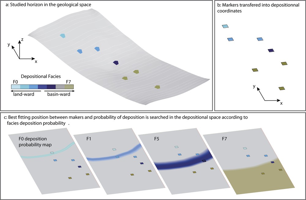
Likelihood computation using theoretical depositional space. A. Studied horizon and makers displaying depositional facies in the geological space. B. Studied markers transferred in depositional space. C. The set of markers is searched in depositional space to maximize the sum of deposition probabilities of each facies.
From this theoretical profile, the correlation cost can be computed as follows:
- • the depth membership function of each facies is used to compute theoretical facies probability maps on the paleogeographic profile (Fig. 7C);
- • on the paleogeographic map, we look for the most likely location of all the markers previously correlated to m1 and m2 (Section 2.4). Let M = {m1,..,mn} denote the set of all these markers, Fi the facies observed at marker mi and the probability of observing the facies Fi at the location of marker mi on the theoretical profile. The most likely location of the markers M on the theoretical map is obtained by finding the horizontal translation of the markers M that maximizes the likelihood of the observed facies (). Because the profile is quite smooth, this position can be assessed by gradient-based optimization.
- • The correlation cost cB(m1,m2) is then computed as (Fig. 6):
| (7) |
In this cost computation, the parametric definition of the bathymetric profile may be influential. Several scenarios for bathymetry or non-parametric profiles computed with process-based models could be used to test concepts and assess their impact on the emerging correlations.
3.2.3 Constraints
The top and bottom horizons of the studied interval (U.I 1 and U.II 6, see Fig. C.10) are input as known correlations to constrain the stochastic well correlation process. This constraint is not a requirement for the correlation method and could be eliminated by defining a null gap cost on the starting and ending correlation, as done for instance by Lallier et al. (2013) for magnetostratigraphic dating. However, this constraint is useful here to compute the correlation costs based on paleo-angles (Section 3.2.1) and the overall stratigraphic geometry of the system.
3.2.4 Results and discussions
3.2.4.1 Geometrical model and grid building
Four possible 3D models were created (Fig. 8B, C, D, and E): a reference model built from the deterministic correlation proposed by Gari (2007) (Fig. 8B) and three models built from the stochastic correlation method (Section 2.4).
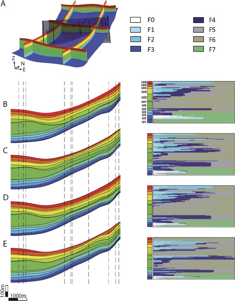
Four possible stratigraphic models for the Cretaceous southern Provence basin. A. 3D deterministic stratigraphic model of the basin (from Gari, 2007). The black lines indicate the location of the studied outcrops; Shaded surface figures the cross-section presented in B–E. B. Stratigraphic correlation model proposed by Gari [2007] and associated vertical facies proportions. Dashed lines are the projected locations of the used outcrops. C–E. Stratigraphic models built from three stochastic correlations and associated vertical facies proportions.
The geometry of these four models is constrained by the geometry of the top and the bottom horizons of the studied interval (U.I 1 and U.II 6, see Fig.C.10). These two horizons were built by Gari (2007) using intersections with the topography and dip and strike measurements in the field. Internal horizons corresponding to well correlations were built so that they respect well markers and the thickness variations of units defined by surfaces are smoothed (Mallet, 2002). A conformable stratigraphic grid was then built for the reference model and the stochastic ones.
The relative visual similarity of some stochastic models with the deterministic interpretation of (Gari, 2007) is reassuring. However, it does not prove that the stochastic model is right (nor that Gari's interpretation is right). Only additional evidence (e.g., from paleontology, palynology or geochemistry) could indicate which of these models are acceptable.
Facies distribution analysis. Statistical facies proportions within each layer were calculated from wells for each stratigraphic model to assess the impact of correlation uncertainty on reservoir properties (Fig. 8). This vertical facies proportion can be analyzed in terms of reservoir facies distribution, considering facies F0 to F4 as potentially reservoir and facies F5 to F7 as flow barriers. Because outcrops located on the north side of the basin display a continuous record of reservoir facies, models built from the stochastic correlations may result in different compartmentalizations of the reservoir. The four models presented in Fig. 8 (representing a small subset of the possible stratigraphic correlation models) show two alternative views of the distribution of reservoir rocks: in the models B and D, reservoir facies are concentrated into two main groups, whereas in models C and E, reservoir facies are divided into several units (6 in model C and 5 in model D) separated by flow barriers. In an actual reservoir study, additional information coming from well production, such as production logging tool could be used to select which stratigraphic correlation models are acceptable.
Considering alternative stratigraphic correlation models may also lead to different interpretations of the sedimentary and tectonic history of the studied area. For instance, Gari (2007) interprets the unit U.I 6 as a prism constituted of marls whose deposition is due to a tectonic tilting. In relation with this tectonic activity, the production of carbonate is stopped on the platform, suggesting a confinement and hypoxic event. In contrast, such a hypoxic event cannot be interpreted if model E is considered, because the equivalent prism is correlated to platform deposits.
4 Conclusions and perspectives
The presented methodology can rapidly generate several possible stratigraphic correlations of a set of stratigraphic sections. These stochastic correlations can be constrained by prior knowledge such as correlation lines extracted from seismic data or/and hypothetical base profile geometry. Several geological scenarios may be tested in agreement with prior geological knowledge.
In the case of carbonate deposits, we have proposed to integrate paleo-bathymetric information to compute correlation likelihood. Many other rules could be considered to define other correlation costs, which could be combined by linear combinations. However, defining costs that have comparable norms and dimensions can be a challenge.
We are currently working towards the definition of additional rules integrating more sedimentological and stratigraphic concepts in carbonate and siliciclastic settings. Indeed, in most depositional settings, the facies type is not controlled only by bathymetry, but also by the distance to the source, water temperature, etc. An interesting area for further research is to better use 3D seismic data when available to address correlation uncertainties. When wells and seismic data are available in the same domain (time or depth), seismic data indeed provide low-resolution correlation trends that should be used in the hierarchical correlation. Another avenue could also be to connect depositional concepts and facies probabilities from seismic attributes (Baaske et al., 2007).
In any case, the validation of such a stochastic method is very delicate. Indeed, the set of possible correlations completely depends on the cost definitions and there is no absolute way of deciding whether it is representative of the uncertainties other than scrutinizing the data and the rules and comparing results with analogs.
Nonetheless, stochastic stratigraphic correlation, combined with geostatistical facies simulation, is a new way to handle uncertainties on reservoir and basin modeling. We see it as complementary to the classical methods performing multiple facies simulation on a unique grid. Further studies would be needed to assess the relative influence of stratigraphic uncertainty and petrophysical uncertainties, and possibly to use inversion to reduce correlation uncertainties.
Acknowledgements
We would like to thank the editors (Philippe Joseph, Pierre Weil, Sylvie Bourquin and Vanessa Teles), Michael Pyrcz and another anonymous reviewer whose comments greatly contributed to improving this paper. This research work was performed in the RING project managed by the “Association scientifique pour la géologie et ses applications” (ASGA). Companies and Universities of the Gocad Consortium (http://www.ring-team.org/index.php/consortium/members) are hereby acknowledged for their support. We also thank Paradigm for providing the Gocad software and API.
Appendix A Combinatorial analysis
Considering two wells with respectively n and m identified stratigraphic markers and assuming that top and bottom markers of each well are correlated together, the number Dn,m of possible correlations between these two wells is given by the Delannoy number (e.g., see Banderier and Schwer (2005)):
| (A.1) |
This equation can be extended in d dimensions, i.e., to enumerate the number of correlations between d wells with respectively ni markers per well:
| (A.2) |
Two simple numerical applications of Eqs. (A.1) and (A.2) highlight the very large number of possible combinations:
- • two wells comprising ten markers each yield D10,10 = 1,462,563 possible correlations;
- • twelve wells comprising seven markers each yield 1080 possible correlation models, which is equivalent to the number of atoms in the universe.
Among this huge set of possible well correlations, only a relatively small subset is likely. Still, even the most likely thousandth of this set cannot be manually appreciated.
Appendix B Correlation ambiguities due to the paleo-angle of a carbonate ramp
The uncertainty on the slope paleo-angle α of a carbonate ramp affects well correlations. (A) Impact of errors in average paleo-angles on the position error of the correlated horizon along the well for different well spacings. Right: for a simple synthetic carbonate ramp (B), an error of 0.05° in the evaluation of the average paleo-angle leads to ambiguities on the correlation of two 10-m-thick units (C). When the angular error reaches 0.15°, the ambiguity is between three such units (D).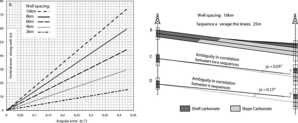
Appendix C Chronostratigraphic and facies information in the Beausset study
Chronostratigraphic and sequence stratigraphic subdivision of the Cretaceous southern Provence Basin. The studied interval is composed of twelve fourth order hemicycles.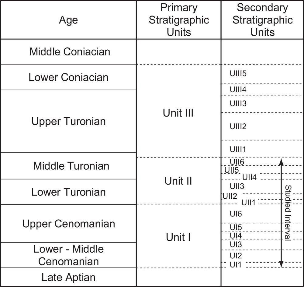
Facies described by their possible depositional bathymetry. This description is used to build the depositional space presented in Fig. 7 and to interpolate the bathymetry along wells. Modified after Gari (2007).
| Facies | Minimum bathymetry of deposition (m) | Maximum bathymetry of deposition (m) | ||
| Value | Uncertainty | Value | Uncertainty | |
| F0: Charophyte limestone | –50 | 0 | 0 | 0 |
| F1: Micritic limestone | 0 | –5 | 1 | 5 |
| F2: Bioclastic limestone with rudists | 5 | 3 | 10 | 5 |
| F3: Bioclastic limestone with rudists and corals | 7 | 4 | 15 | 5 |
| F4: Bioclastic limestone with fragment of rudists and corals | 15 | 5 | 50 | 10 |
| F5: Argillaceous limestone | 50 | 25 | 100 | 25 |
| F6: Marl and marly limestone | 125 | 25 | 175 | – |
| F7: Brecia, lobe, grainflow and debris flow | 40 | 10 | 175 | – |