

1 Introduction
Several recent oil discoveries are set in deep-marine reservoirs, and these are commonly composed of turbidite sandstones with very good reservoir properties, but also with a very high degree of heterogeneity. These reservoirs are usually formed by the stacking of deposits related to several hundreds of individual turbidity flow events. There is a wide range of gravity flow types and several classifications have been proposed in the literature according to flow characteristics such as rheology or density (Mulder and Alexander, 2001; Mulder and Cochonat, 1996; Shanmugam, 2000), sedimentary facies of deposits (Mutti and Ricci Lucchi, 1975; Pickering et al., 1989) or sediment transport processes (Lowe, 1979; Middleton and Hampton, 1973; Stow et al., 1996). The relationship between processes and resulting architectures are still subject to debate (Mulder, 2011; Shanmugam, 2012), particularly because direct observations and characterization of turbidity currents are difficult in reality. They are the scene of several complex physical processes interacting in a nonlinear way. Even in recent cases such as turbidity currents monitored in Monterey Canyon (Xu et al., 2004, 2013), and the 1929 Grand Banks event (Piper et al., 1999) or the 1979 Nice event (Migeon et al., 2001; Mulder et al., 2012), where cable breaks provide constrains on timing and associated deposits can be studied, there is debate on the flow regime, transport and deposition processes.
Most of these reservoirs lie in deep-offshore locations where data are scarce. To better understand their internal architecture and sediment distribution, one approach is to study the processes, which led to their formation. Numerical modeling is one way to study these systems and to link the modeled processes to the associated deposits and resulting architecture. All parameters can be easily controlled and sensitivity analysis can be carried out. The difficulty lies in modeling the different processes and their interactions correctly when there is still debate on the acting processes themselves and on the different proposed formulations. The most detailed flow models (Basani et al., 2014; Meiburg et al., 2015; Rouzairol et al., 2012) implement 3D Navier–Stokes equations and are able to reproduce the full complexity of turbulent flow. But, these detailed numerical simulations require huge running times, even with highly parallelized powerful computing machines. The most common approximation of the Navier–Stokes equations is the Saint-Venant system of equations (e.g., Parker et al., 1986; Zeng and Lowe, 1997) in which the flow parameters are depth-averaged. Even with this approximated approach, the application of these models to a whole turbidite reservoir, resulting from the stacking of many flow event deposits, remains a challenge. Furthermore, since flow parameters vary from one event to the other and are difficult to infer from field data, it is difficult to constrain the model with accurate parameters. The applications of such process-based models follow a trial-and-error approach that requires several simulations and thus high computation time.
To overcome these problems, an alternative approach is to use simplified models mimicking the flow with enough realism to reproduce detailed description of reservoir architecture and heterogeneity of deep-offshore fields and with low computation times in order to generate multi-event simulations. To this purpose, the Cellular Automata for Turbidite Systems (CATS) model was developed at IFPEN. CATS is a multi-lithology process-based model for turbulent turbidity currents and their associated sedimentary processes. An overview of CATS capabilities in different contexts is presented and discussed in this paper.
2 Model description
2.1 CATS: a model for low-density turbidity currents
Among gravity flows, turbidity currents are usually defined as submarine sediment-laden flows in which the transport is mainly supported by the flow turbulence, with a distinction between high-density and low-density turbidity currents (Middleton and Southard, 1984; Mulder and Alexander, 2001). The CATS model has been developed for low-density turbidity currents where sediments are transported essentially in suspension by the fluid and where interactions between particles can be neglected. Mulder and Alexander (2001) give a maximum threshold of 9% of volumetric sediment concentration for low-density turbidity currents above which interactions between particles become non-negligible (Bagnold, 1962). In such a context, the main processes to be modeled are sediment-laden gravity-driven flow of turbulent dilute sediment suspensions, ambient water entrainment into the flow and sedimentary processes such as erosion and deposition.
2.2 Cellular Automata principles
This model is based on cellular automata (CA) concepts (Salles, 2006):
- • the space is partitioned into identical cells composing a regular mesh. Each cell is an automaton and bears the local physical properties of the flow and of the seafloor;
- • the chosen modeled processes are implemented through local laws either as local interactions between neighboring cells through mass and energy transfers; or as internal transformations of physical and energetic properties in each cell, which can be performed independently from the neighbors’ state.
In the CATS model, flow distribution driven by gravity and by kinetic energy is considered as local interactions between adjacent cells. Sediment erosion, deposition and water entrainment of ambient water are internal transformations essentially based on empirical laws.
2.3 The flow model
2.3.1 Definition of the flow
The flow is described by a thickness (h) representing the turbiditic sediment-laden flow thickness, by volumetric mean concentrations (Csedi) of different chosen discrete lithologies, and by a scalar velocity U (in m/s) computed from the kinetic energy balance in the system. It means that there is no vector velocity that could drive the fluxes and could define their direction. The ambient fluid is not explicitly modeled. Sediments are defined in as many discrete classes of particle types (grain-size and composition, referred to as “lithology”) as needed to describe the sedimentary system. Secondary variables such as particle settling velocity are computed following empirical laws (Dietrich, 1982; Soulsby, 1997). Others, such as critical erosion/deposition shear stress can be adjusted by the user to model different sediment behaviors and change their erodibility or depositional capabilities. The seabed is described by a given topography (cell altitudes) and proportions of the different sediments.
2.3.2 Flow distribution: a local algorithm
The CATS model is inspired by the cellular automata approach first developed by Di Gregorio et al. (1994, 1997, 1999) for subaerial landslides where the flow distribution is computed through the local algorithm of “minimization of height differences”. Salles (2006) and Salles et al. (2007) adapted this algorithm for submarine turbidity currents. The algorithm seeks the equilibrium of energies between neighboring cells, considering both potential and kinetic energies, in order to take into account both gravitational and inertial effects. They are represented respectively through the flow thickness at the cell elevation and through the run-up height (hr). The latter was first defined by Rottman et al. (1985) as the height that can be reached by the flow when its kinetic energy is transformed to an equivalent potential energy. In CATS, the run-up height is a function of the scalar flow velocity U:
This distribution is done by computing, with an explicit scheme, volumes to be output per iteration (called “outfluxes” in the text hereafter) from every cell to each one of the four neighboring cells. Details of the flow thickness distribution algorithm are presented in Supplementary material 1.
After computation of these outfluxes for all cells of the computational grid, the flow parameters are updated according to overall mass and energy conservation principles, taking into account the transfers between cells, and the transformation between kinetic and potential energies (see details in Supplementary material 2).
This algorithm is similar to a local diffusion process applied to both kinetic and potential energies. The flow behavior is controlled by the topography, the flow thickness and kinetic energy. On high slopes, the flow will follow the topography gradient and will propagate downslope. On low-gradient topographies, the flow distribution will tend to spread in all directions as an isotropic diffusion of the flow thickness. The use of the run-up height in the algorithm allows the flow to climb upward by inertia according to its kinetic energy.
2.3.3 Sediment concentration transfer
In nature, the vertical sediment concentration profiles in the flow are very different, depending on the particle size distribution and density (Kneller and Buckee, 2000). Moreover, in complex topographies, the distribution of coarse or fine sediments carried in suspension can be quite different (Altinakar et al., 1996; Parker et al., 1987). Fine-grained sediments can easily be distributed throughout the whole water column, and show an almost homogeneous concentration along the vertical and, thus, will be distributed more easily on topographic highs such as terraces or levees when the flow spills over. Conversely, coarse-grained sediments are more concentrated toward the bottom of the flow and will tend to remain in topographic lows such as channels. These different sediment distributions in the flow are important to consider in order to correctly reproduce the resulting deposited sediments.
In order to take into account these different behaviors in sediment transfer with the flow, CATS computes vertical concentration profiles with different shapes depending on the sediment grain-size and density. In the following balance equation at equilibrium (Glenn and Grant, 1987; Soulsby, 1997), the settling of the grains toward the bed is counterbalanced by the diffusion of grains upward, due to the turbulent water motions near the bed:
- • ws,i is the settling velocity for each lithology i,
- • Ci (η) is the suspended-sediment concentration of lithology i at elevation η above the sea floor and
- • Ks is the eddy diffusivity. It depends on the turbulence in the flow, through the shear velocity u*, on the elevation above the seafloor η and on the flow thickness h (Rouse, 1937):
the Rouse number (κ is the von Karman constant = 0.40) and
- • Ca,i is a reference suspended-sediment concentration at elevation η = ηα (see Smith and McLean (1977) for details).
Different concentration profiles can be obtained as a function of the Rouse number (Fig. 1).
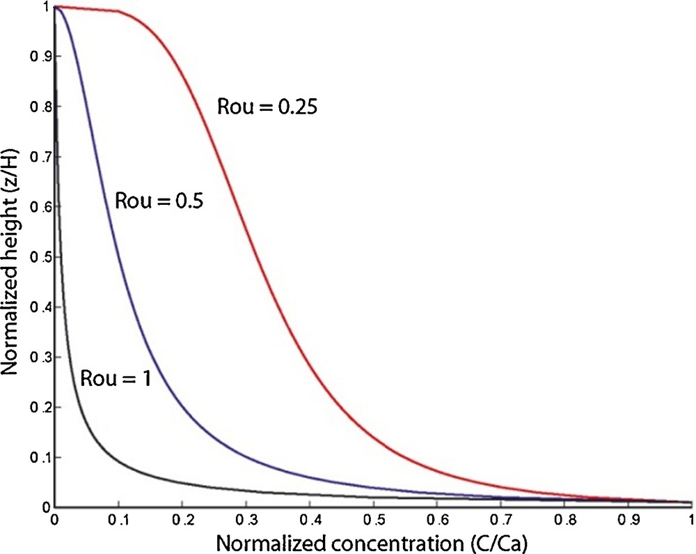
Normalized suspended-sediment concentration profiles for three different Rouse numbers.
For small or light sediments and strong current, the Rouse number is low and the vertical concentration tends to be constant vertically as the flow turbulence can easily maintain them in suspension. Conversely, for coarse or heavy sediments and weak current, the Rouse number tends to one and the sediments are concentrated mainly near the bed.
Sediment transfer capacity is computed according to the computed “Rouse profiles”. If the value of the Rouse number is small, the sediment concentration is homogeneous over the whole water column and the sediment concentration of the transferred water mass will be very close to the mean sediment concentration in the flow. In the case of a flow distribution to a higher neighbor cell, only the upper part of the water column that spills over the obstacle is transferred. For coarser sediments, the concentration will be significantly lower than the mean concentration of the whole water column (see section 3.1.1 for an illustration of differentiated sediment distribution).
2.4 Water entrainment process
The turbulent turbidity flow thickness tends to grow with distance downstream through the incorporation of ambient fluid (Ellison and Turner, 1959). The water entrainment coefficient (ew) is commonly expressed empirically as a function of the Richardson number (Ri), which is defined as the ratio of the work done by gravity to the work done by inertia: (Fukushima et al., 1985; Parker et al., 1987; Turner, 1986). The Ri number is the inverse of the square of the densimetric Froude number.
In the work, the entrainment is computed according to Turner's (1986) law, identified from the laboratory experiments of Ellison and Turner (1959):
Wells et al. (2010) have compiled the available information on the entrainment ratio, extending this previous range. They showed that the entrainment ratio asymptotes to 0.08 for low values of Ri. Water entrainment leads to an increase in the flow thickness and a decrease in the flow concentration. In addition, the dissipation of kinetic energy linked to this process is applied and estimated according to the entrainment rate ew.
2.5 Sedimentary processes: erosion and deposition
Similarly to water entrainment laws, erosion and deposition laws are empirical and originate from laboratory studies performed to characterize the physical processes governing turbidity currents (Hiscott, 1994; Partheniades, 1971). All these empirical laws may be controversial as they are deduced from different specific analogue models that have their own experimental protocol and are deduced from laboratory scale experiments and applied on a mesoscopic scale (grid space).
Furthermore, there is still debate on what the flow parameters controlling erosion and deposition laws are. It is common to relate observed deposited grain-sizes with flow velocity as the main control of the flow competence for transporting sediments. One type of law is to compute erosion and deposition by comparing the flow shear stress to critical values of the shear stress for different lithologies (Krone, 1962). However, Hiscott (1994) proposed that deposition is not controlled by the flow competence (velocity), but rather by the capacity of the flow to carry, in suspension, its sediment load composed of several sizes of particles. That would explain the discrepancies raised by Komar (1985) in the velocity estimates from observed deposit grain-sizes. Flow competence and transport capacity are two different ways to apprehend erosion and deposition processes. This question is very similar to the one still in debate in fluvial and landscape evolution communities between transported-limited versus detachment-limited approaches (Pelletier, 2011). The relative importance of one concept versus the other is probably case-dependent, according to the flow regime and the sediment types, among other parameters. Thus, both approaches are implemented in the CATS model and can be used according to the user's understanding of his study case.
2.5.1 Erosion and deposition laws as a function of flow shear stress
Partheniades’ (1971) erosion law and Krone's (1962) deposition law both depend on the difference between the flow basal shear stress and the critical shear stress defined for each lithology.
In CATS, the bottom shear stress is computed as a function of the current density (ρc), the flow velocity (U) and the drag coefficient (CD ∼ 10−3–10−2) by the quadratic friction law (Soulsby, 1997):
The critical shear stress value of a given lithology can be either computed according to the Soulsby and Whitehouse (1997) law or set directly by the user.
The rate of erosion E is computed for each cell and for each lithology using Partheniades’ (1971) law for cohesive sediments:
Deposition occurs when the value of the flow shear stress on the bed (τb) is lower than the critical shear stress defined for each lithology i. It is a function of the “settling velocity” (ws,i) and of the effective concentration Ceff,i computed in the flow bottom layer hdep that can potentially contribute to deposition during the current computational time step:
2.5.2 Erosion and deposition laws as a function of flow capacity
The flow capacity Ccap is defined as the maximum theoretical amount of sediment that can be transported in the flow suspension at a given mean velocity. It is computed as the integral of the Rouse concentration profile described in Section 2.3.3 following the approximated solution proposed by Hiscott (1994). The cell concentration value Csed is compared to this flow capacity Ccap (Fig. 2).
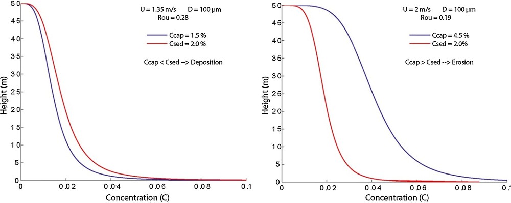
Maximum sediment transport capacity (blue line) and sediment concentration in the water column (red line). Left: if sediment transport capacity becomes smaller than the concentration in the water column, after flow deceleration for example, deposition is activated so that Csed returns back to Ccap value. Right: if sediment transport capacity becomes larger than the concentration in the water column, after flow acceleration for example, erosion is activated so that Csed tends to Ccap.
If the flow capacity Ccap is greater than the current flow concentration Csed, the “Rouse” erosion rate is applied and more sediment is eroded from the bed and put into suspension in the water column, so that Csed tends to Ccap. The formulation of the erosion rate is then identical to Partheniades’ (1971) law. No erosion will occur if the flow concentration is at its full capacity Ccap, even if the bottom shear stress is much higher than the critical shear stress for grain motion.
If the flow capacity value Ccap becomes smaller than the flow concentration Csed, due to a flow deceleration for example, then the excess sediment can be deposited so that the sediment concentration tends to the theoretical concentration value Ccap. The definition of the deposition rate depends on the excess of sediment concentration to the flow transport capacity. It can be written as follows:
3 Applications
Several applications of CATS are presented in this section in order to illustrate the different capabilities of the model on complex topographies. Albertão et al. (2014) show an application of CATS to an ancient subsurface case in the Brazilian offshore.
3.1 Synthetic sinuous channel and unconfined topography
The first series of simulations of the CATS model are performed on a synthetic inclined sinuous channel opening on an unconfined flat area (see Fig. S1, Supplementary material 3). The grid is 3 km wide and 7.5 km long, with a 50 × 50 m resolution. The upstream part of the simulated domain features a 25-m deep and 400-m wide sinuous channel with a sinuosity of 1.32 and a slope of 0.5°. The downstream part is a 3 × 3-km-flat unconfined topography. The main purpose of this simulation is to show the spatial distribution of different lithologies that can be achieved when using the Rouse profile. A first single-event simulation performed with the Rouse approach is described in Supplementary material 3. It shows a realistic deposit distribution on the topography: the coarser lithology is confined in the channel, whereas the finer one is able to overspill and deposit on the banks.
3.1.1 Multi-event simulation
On the same topography, a multi-event simulation with 50 events was performed with different initial sediment concentrations in the flows (Maktouf, 2012). Each flow event is active during 6104 s (16 h 40 min) with constant values of flow thickness and velocity respectively equal to 10 m and 2 m/s, and varying sediment concentrations. The scenario of turbidity current events has been chosen in order to mimic a progressive decrease of the sand supply (following a by-pass stage not simulated here), corresponding to the first 40 events, then a reactivation of the sand supply (last 10 events) (values of input flow thickness, velocity and sediment concentrations for each of the 50 events are illustrated in Fig. S3, Supplementary material 3).
The flow values were calibrated in order to obtain aggrading channel deposits and a lobe in the unconfined area at the mouth of the channel. Sand and silt lithologies were defined as in the previous simulation (see Table S1, Supplementary material 3).
Erosion and deposition processes were modeled with the shear stress-dependent laws described in Section 2.5.1. The other parameters are the same as in the previous single-event simulation, except for the concentration profile, which is considered to be constant for all lithologies in this simulation.
The first flow stays confined in the channel, its thickness increases up to 20 m due to water entrainment. On the unconfined area, the flow spreads out, leading to a decrease of the flow velocity and to lobe-shaped deposits. In the channel, once the flow input ends, sediments are deposited in a relative homogeneous layer, with a thickness of 0.6 m in the upstream part of the channel, decreasing downstream to 0.2 m in the lobe. The parameters were chosen to simulate the gradually filling in of the channel by successive events as in an abandonment process. The simulated flow, first channelized, overspills as the simulation progresses and creates levees on the channel banks. Fig. 3 illustrates the simulated deposits through time every 10 flow events. Sands and silts are deposited in the channel with a fining upward during the first 40 flow events due to the fining of the input concentrations in the flow. In the unconfined area, cross-sections show that the simulated deposits of the last 10 events (which correspond to a new phase of sand input) are diverted to the right (Fig. 3, bottom). The previous deposits on the unconfined surface at the channel mouth have decreased the local slope in the channel's axis. The flow is diverted and follows the higher lateral slope gradient, in processes similar to the lobe compensation process proposed by Mutti and Sonnino (1981).
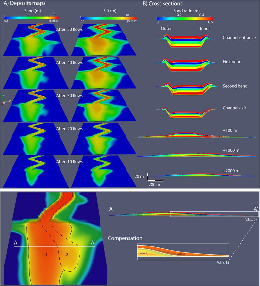
Top A: simulated sand and silt deposit maps output at the end of each 10 flow event sequence (from bottom to top panels). Color bars are in log scales. Top B: Final simulated deposits in cross-sections at each channel bend and through the unconfined deposits. Bottom: 3D map and cross-sections highlighting the compensation-like lobe deposits.
3.2 Makran topography
This second application based on a real present case illustrates the ability of the CATS model to simulate the behavior of turbidity currents on a complex topography and the prediction of the related deposits. In the northwestern part of the Oman basin, the offshore part of the Makran accretionary wedge is composed of several accreted ridges and piggyback basins (Ellouz-Zimmermann et al., 2007). A dense system of canyons and gullies cuts across the Makran prism. These systems have been characterized by Bourget et al. (2011) from the data acquired during the CHAMAK cruise (Ellouz-Zimmermann et al., 2007). They found that these networks converge downstream in seven outlets, thus defining seven canyon systems. The model has been applied to the downstream part of the second canyon system described by Bourget et al. (2011) (Figure S4, in Supplementary material 4). The “Makran” topography dimensions are 12.4 km in width and 38.4 km in length with a grid resolution of 400 m × 400 m. The average slope is 1.6°. The upstream part of this topography shows the end of a wide sinuous canyon opening into a small basin confined by the last accretionary ridge (Bourget et al., 2011). It connects downstream to a plunge pool which is 15 km long, 7 km wide and 150 m deep through a 400-m-high “knickpoint”, defined here as a disruption in the equilibrium due to the last accretionary ridge, as in Bourget et al. (2011).
On this real complex topography, 150-m-thick flows are input at the most upstream point of the canyon available in this topography (white arrow in Fig. 4). Two types of flow are simulated: the first one has a finer sediment load (composition: 2% of fine silt and 1% of sand), while the second one is sandier (composition: 1% of fine silt and 3% of sand). Both are dilute flows below the Bagnold limit of 9% (Middleton and Hampton, 1973). Sediment characteristics and simulation parameters are detailed in Table S2, Supplementary material 4. The multi-event simulation is composed of 25 events (10 ‘muddy’ flow events, 10 ‘sandy’ flow events and then 5 ‘muddy’ flow events) (see Table S2, Supplementary material 4 for simulation details).
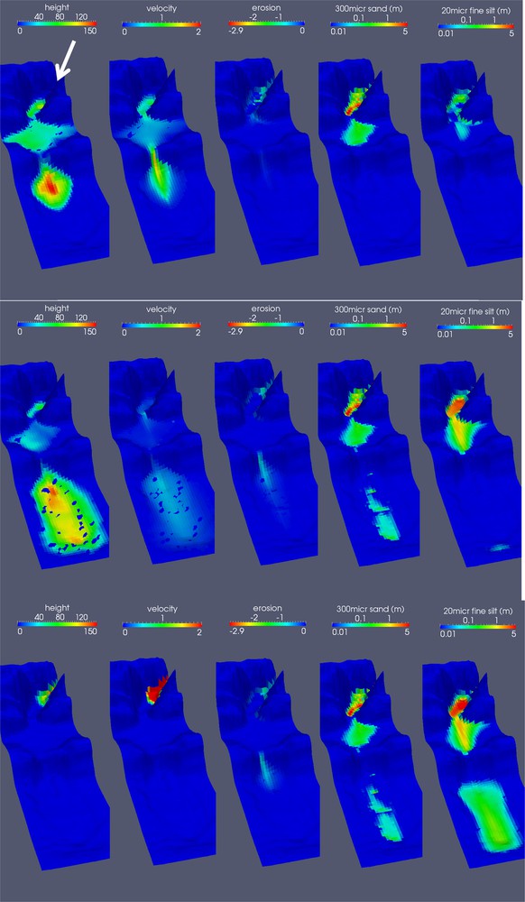
Simulation results showing from left to right: Flow thickness (height in m), flow velocity (m/s), erosion of the substratum (m), sand and fine silt deposits (m). (Color bars for deposits are in log scale, vertical exaggeration × 7). Different stages of the simulations are shown. Top: During the first event, when the flow reaches the second basin passing the last accretionary ridge, velocity increases and leads to erosion (visible on the middle panel). Middle: The flow spreads over the whole domain, sands are deposited in the plunge pool, fine sediments start to deposit on the downstream bank. Bottom: At the beginning of the second flow, showing the different distributions of the two types of sediments over the topography.
The simulated flow is first channelized by the canyon walls. Due to the run-up height and the Rouse profile, the flow climbs a little on the sides where it decelerates. This leads to the deposition of fine-grained sediments first on the sides, whereas the coarse-grained sediments are deposited in the middle of the canyon. When the flow spreads in the first basin, its velocity decreases, leading first to the sedimentation of sand just past the canyon mouth, and then to the deposition of fine silts farther in the basin. Part of the flow is able to exit the domain laterally in this unconfined basin. When the flow reaches the knickpoint, it is channelized towards the plunge pool and accelerates, leading to erosion in the slope (Fig. 4, top panels). In the plunge pool, sands deposit first inside the pool, and silts start to deposit on the downstream bank of the pool (Fig. 4, middle panels). With a flow input activity of 8000 s, the flow is able to reach the downstream boundary of the computational domain over-spilling the plunge pool banks, but at that time, the flow is already waning. Flow velocity decreases and, with it, the flow capacity and shear stress reaches the decantation point successively for each lithology leading to the sedimentation of the remaining sediments in the flow column. The bottom panels of Fig. 4 show the simulation results at the beginning of the second flow: flow height and velocity are visible in the canyon. Sand and silt were deposited by the first flow. They show a different spatial distribution, with sands confined within the plunge pool and silts deposited downstream. The difference in deposits between the middle and bottom panels is due to the decantation process at the end of the flow.
The CATS model is able to simulate both erosion of the initial topography (erosion panels on Fig. 4) and remobilization of the previous deposits.
Fig. 5 shows the sand proportion of the simulated deposits along the plunge pool at the end of the 25 flow events. No seismic cross-section is available for this specific location. However, it is possible to compare the resulting main sedimentary features with the seismic line across a close-by plunge pool published in Bourget et al. (2011). They recognized “distal plunge pool deposits that aggrade and migrate” in the downstream direction, they “onlap and form the plunge pool flanks.” (Bourget et al., 2011) These features are very similar to the distal deposit in the plunge pool of the simulation (Fig. 5). Bourget et al. (2011) also identified mass wasting and locally sharp erosional surfaces in the most proximal banks of the plunge pool just after the “knickpoint”. The CATS model simulates erosion in the slope and just downstream the accretionary ridge. Note that each flow event starts with erosion and remobilization of previous deposits farther downstream. The last 5 “muddy” events produce a blanketing of the system.
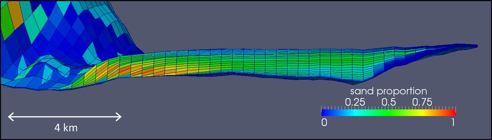
Cross-section in the simulated multi-event deposits along the longitudinal axis of the plunge pool (vertical exaggeration × 10). The flow direction is from left to right.
4 Discussion
The CATS model is able to simulate several multi-lithology gravity-driven turbidity flow events associated with sedimentary processes such as erosion, deposition and water entrainment of ambient fluid. The simulations show that the modeled processes are able to reproduce complex deposits using simple laws that control local and internal interactions of the cells. The flow is distributed according to an algorithm similar to the diffusion of energy. On high slope topography, the simulated behavior is controlled by the local slopes and matches well the expected turbulent flow behavior, which follows the highest slope gradients. These local rules are adapted to fast computation solutions. The single flow events presented here are computed in a few minutes on several processors. Complex behavior and feedback between processes seem to be accurately simulated.
As the flow distribution is mainly controlled by the local slope, the model is not able to reproduce an advective flow on a flat or low-slope surface. In this specific case, the diffusive behavior will always be dominant, spreading in all directions, and will not accurately reproduce the advection part of the flow on low-slope topographies. This issue is related to the computation of time step for each iteration of the cellular automata approach that infers, following Salles (2006), that the process velocity can be inferred from the kinetic energy , whereas the computed outfluxes are computed through the more complex flow distribution algorithm (see Supplementary Material 1). Several tests have shown that this time step needs to be adapted to the cellular automata actual flux computation. Developments are in progress to tackle this issue.
5 Conclusion
The CATS model is a process-based model intended to simulate turbulent low-density turbidity flows. It is based on cellular automata concepts and implements an algorithm of local diffusion of energies coupled with other physically- or empirically-based processes such as sediment concentration profiles controlled by the Rouse number, and erosion, deposition and water entrainment laws.
The objective of such a modeling approach is to reproduce the architecture and spatial distribution of the facies of turbidite reservoirs with a physical consistence given by the simulated sedimentary processes. The second objective is to perform fast simulations that can be integrated in operational workflows of the petroleum industry. The model has been applied to different settings: synthetic channel and unconfined topographies and real-world complex topographies. It shows realistic transient behaviors and the resulting distribution of coarse and fine sediment deposits.
Acknowledgments
The authors would like to thank sponsors of the CATS JIP project in IFPEN (Engie, Petrobras, Statoil, DONG Energy, BHP Billiton, Total), who supported part of the development of the CATS model. They would like to thank also Ben Kneller (University of Aberdeen) and Richard Labourdette (Total) for their constructive reviews, which helped them to improve this paper.