

1 Introduction
1.1 The problem
Increasing necessity in drinking water requires delineation of saline aquifers to avoid vain expensive drilling. It has led to the development of invasive geophysical (mainly, electromagnetic) methods enabling to reach deep aquifers and study their physical parameters (Guérin et al., 2001; Levi et al., 2008). That is why the determination of the relationships between the physical parameters of saline to hypersaline aquifers and groundwater salinity remains a challenge. Moreover, the environmental impact associated with such kinds of groundwater is undeniably a worldwide problem.
Evaluation of water salinity is especially important in coastal regions, because an intrusion of salt water from the sea into the mainland may significantly deteriorate fresh water quality (Goes et al., 2009). Evaluation of water salinity is mainly based on interpreting the bulk resistivity of aquifers measured by surface geoelectrical methods using either methods of direct current, e.g., Vertical Electric Sounding (VES) (i.e., Kirsch, 2006; Koefoed, 1979) or the Transient Electromagnetic (TEM) method, also called Time Domain Electromagnetic (TDEM) soundings (i.e. Chalikakis et al., 2011; Descloitres et al., 2011; Fitterman, 2014; Guérin et al., 2001; Levi et al., 2008). The use of resistivity methods for the estimation of water salinity is based on the dependence of the bulk resistivity (ρx) of the aquifer on the resistivity of the fluid filling its pores (ρw) and on porosity (φ). This dependence is expressed by Archie's law (Archie, 1942), which we will consider below.
In accordance with a hydrogeological model (Yechieli et al., 2001) in the Dead Sea region (Fig. S1), the recent drop in the sea level and the associated drop of fresh-saline water interface allow the incursion of fresh groundwater coming from the west or from deep layers via faults into the coastal aquifer. When the DS level was high, groundwater was similar in composition to the DS water, with total dissolved solids (TDS) approaching ∼340 g/l.
Lowering of the DS level and migration of chemically undersaturated (in relation to halite) groundwater into the coastal aquifer has caused diverse environmental changes (such as landslides, land subsidence, disturbance of coastal springs etc.) via the variation of the groundwater salinity, resulting in the dissolution of the buried salt layers and, most significantly, in wide-scale collapse and sinkholes development above the salt (Closson et al., 2010; Salameh and El-Naser, 2000; Yechieli et al., 2006).
Thus, estimating the groundwater's salinity and its spatial distribution (mapping) as well as monitoring is of a high importance for the quantification of its dissolving potential associated with the DS sinkhole problem.
1.2 TEM method: efficiency and use around Dead Sea
The transient electromagnetic (TEM) method is sensitive specifically to the bulk resistivity (conductivity) of the studied medium, especially in the low resistivity range. The TEM method is used in hydrogeology mainly for sounding, i.e. for investigating layered structures below the surface. The TEM method has been routinely used in Israel for 25 years for locating the fresh water–saline water interface in coastal areas of the Mediterranean, Red, and Dead Seas to delineate salt water intrusions into coastal areas (Goldman et al., 1991). A number of researchers (Kafri et al., 1997; Levi et al., 2008; Yechieli et al., 2001) have suggested to classify the Dead Sea aquifers based on bulk resistivity determined through TEM measurements (see review in Supplementary section S1).
In conditions of high-salinity, the TEM method has a number of advantages compared with Vertical Electric Sounding (VES). (1) TEM enables to study very highly conductive targets like sea brine, whereas direct current (DC) of VES is screened by the very high conductive medium (McNeill, 1980a). (2) TEM sounding allows one to reach deeper levels at less Transmitter–Receiver (T/R) separations than it does in all conventional, controlled source methods. As a result, TEM is the only method in electrical prospecting that permits a T/R separation less than the depth to the target, a feature which, in turn, markedly improves the lateral resolution of the method (Goldman et al., 1991; Guérin et al., 2001). Finally, (3) at corresponding conditions (the late stage of the transient), TEM possesses the highest resolving capabilities in comparison with the DC method, which is mostly sensitive in highly resistive environments (Kaufman, 1978).
However, previous studies intended to classify the Dead Sea aquifers based on bulk resistivity have several limitations: (1) the boreholes previously used for the calibration of TEM results in the DS region were mainly located several kilometers away from the shoreline (Yechieli et al., 2001). The studied resistivity–salinity relationships range from 1 Ω·m upward (Kafri and Goldman, 2006), whereas at the area of interest the bulk resistivity of brine-saturated sediments starts at 0.2 Ω·m. Therefore, more accurate calibration of TEM data is required for interpreting TEM resistivity in terms of groundwater salinity in the DS coastal areas. (2) In addition, the researchers mentioned above were dealing exclusively with sandy aquifers, whereas silty aquifers are very common, particularly at the recently exposed DS shores. Finally (3), salt dissolution in the sinkhole development areas takes place at very low (ρx = 0.5–0.6 Ω·m and less) bulk resistivity values of the groundwater enveloping the salt layer from above and from below (Fig. S1) (Ezersky et al., 2011; Yechieli et al., 2006); this phenomenon should be investigated.
1.3 Goal and objectives of the study
The main goal of the present study is the evaluation of the groundwater salinity (Ccl) based on surface TEM measurements of bulk resistivity (ρx). The objectives of the study were to evidence, respectively:
- • the relationships between groundwater salinity (Ccl) and resistivity (ρw);
- • the relationships between the salinity (Ccl) of the water filling the pores of the aquifer and its bulk resistivity (ρx).
The objectives of the study are resolved based on borehole investigations and near-located TEM measurements.
2 Geology and hydrogeology of the Dead Sea coast
The Dead Sea is the terminal lake of the Jordan River system, nowadays located 428 m below sea level (b.s.l.) in an extremely arid environment, with an annual precipitation of 50–100 mm. Since the early 1960s, the Dead Sea's level in the northern basin is continuously falling, recently at a rate of about 1.0 m/yr. The southern Dead Sea basin (named also Evaporation Ponds–EPs) is kept inundated by water from the Dead Sea pumped from the northern basin. The Eps’ level is artificially maintained at ∼395 m b.s.l. The survey areas are located between the Dead Sea's shoreline and the western border of the Dead Sea's rift (Fig. S1). In these areas, mostly situated on alluvial fans, the surficial deposits are composed of Holocene sediments consisting of sandy-gravels (from pebbles to boulders), and of lime carbonates overlying and underlying a 10–30-m-thick salt layer located at depths between 25 and 50 m. The sandy-gravel sediments lime carbonate (mud) is made up of about 95% of clay to silt sized calcite, with the other 5% being authigenic aragonite, quartz, and gypsum (Frydman et al., 2008). These sediments were deposited by seasonal floods and DS water.
The DS salt layers of Early Holocene age are very conductive hydraulically and water saturated with very highly saline Dead Sea brine with amounts of total dissolved solids [TDS] of 340 g/l (up to 380 g/l in the southern basin) (Yechieli, 2000; Yechieli et al., 1995). The hydrogeological conditions have been thoroughly described by Yechieli et al. (2006). The chemical composition of the DS water and groundwater in boreholes is presented in Table 1.
Chemical composition of ground water from two wells, DS and EP.
| Well | Depth | Na, g/l | K, g/l | Ca, g/l | Mg, g/l | Sr, g/l | Cl, g/l | SO4 | Br, g/l | TDS, g/l | NaCl, g/l | Other solids |
| Mn-2a | 20 | 67.0 | 5.3 | 9.9 | 28.0 | 0.15 | 205.4 | 1.20 | 3.70 | 320.65 | 272.4 | 48.25 |
| Mn-2a | 30 | 75.7 | 4.6 | 11.30 | 22.8 | 0.18 | 202.0 | 1.10 | 3.20 | 320.88 | 277.7 | 43.18 |
| EB2a | 28 | 25.7 | 8.4 | 19.8 | 50.4 | 0.36 | 230.7 | 5.65 | 341.11 | 256.5 | 84.61 | |
| EB2a | 40 | 30.6 | 6.7 | 18.1 | 47.6 | 0.32 | 223.9 | 5.43 | 332.65 | 254.5 | 78.15 | |
| DSb | 40.1 | 7.65 | 17.2 | 44.0 | 224.9 | 0.45 | 5.30 | 339.6 | 265.0 | 74.6 | ||
| EPb | 16.7 | 11.1 | 25.2 | 62.3 | 258.9 | 0.29 | 7.47 | 381.96 | 275.6 | 106.36 |
The density of the DS brine is 1230 kg/m3 in the northern basin and ∼1240 kg/m3 in the EP. Dead Sea water also has very high chloride (Cl–) concentration (up to 224 g/l), which constitutes 98% of the anions, with little sulfate and carbonate. Chloride concentration is therefore the main parameter used to characterize the groundwater's salinity (Yechieli, 2000), especially taking into account the direct practically functional dependence between chlorides (Cl), sodium chloride (NaCl), and the total dissolve solids (TDS).
A number of observation boreholes have been drilled by the GSI along the Dead Sea coast (Yechieli et al., 2004). These boreholes are located in eight sites (Fig. S2). The chloride concentration (Ccl) of the groundwater varies mainly from 120 to 238 g/l, which corresponds to 54–93% of saturation.
The DS coastal areas have been dramatically hit by sinkhole phenomenon occurring since the late 1980s (Fig. S2b, c). Most researchers relate the sinkhole phenomenon with the formation of dissolution cavities within the salt layers with consequential gradual collapse of surface sediments (Ezersky, 2006; Frumkin, 2013; Yechieli et al., 2006). The continuous drop of the DS level at a rate of ∼1 m/yr is generally proposed as the main triggering factor. The lowering water table induces a gradual collapse of shallow unconsolidated sediments overlying buried cavities formed within the salt layer.
3 Water salinity evaluation using Archie's law
In sandy aquifers, the resistivity of the subsurface generally depends on several parameters, among which the most important are the salinity of the fluid in the pores and porosity. The quantitative interpretation of the results can be based on Archie's law (Archie, 1942; Keller and Frischknecht, 1966), which empirically establishes that in physically saturated sandy (clay free) sediments with conductive water in the pores, the bulk electrical resistivity of the aquifer depends on porosity, the resistivity of the pore fluid, and the geometry of the pores.
In this case, the bulk resistivity is expressed as:
| (1) |
Archie's law states that the ρx/ρw ratio (called the formation factor F) is constant at constant porosity and without change in pore geometry. It follows from Eq. (1) that there is a direct dependence between ρw and ρx measured by the TEM method. The formation factor F is a function of water salinity as measured by chloride concentration or total dissolved solids (TDS). F ranges between 1 and 100 and over (Keller and Frischknecht, 1966). In sandy clay free aquifers, this relationship allows the interpretation of bulk resistivity in terms of salinity, providing a determination of porosity and of parameters a and m. Addition of clay to the sandy aquifer complicates such interpretation. Clay minerals (kaolinite, halloysite, montmorillonite, etc.) change, by means of the cation exchange capacity (CEC) effect, the bulk resistivity (conductivity) of aquifers as predicted by Archie's equation (Keller and Frischknecht, 1966; McNeill, 1980b).
It follows also from Eq. (1) that generally it is impossible to use only TEM measurements for determining both water resistivity and porosity (φe). Usually, the parameters ρx and φe are not known, and one of them is assumed to be constant throughout the investigation area. When porosity can be presumed to be constant, water salinity will be calculated directly from bulk resistivity (Goldman et al., 1991). When salinity can be fixed, Archie's law enables to calculate porosity (Kafri and Goldman, 2005). When this assumption is not valid, some additional information about the geological formation (for instance, from boreholes) is required to correctly interpret the TEM data in terms of formation salinity. To solve this problem, attempts are made to combine geoelectrical methods with either MRS or borehole logging (Legchenko et al., 2009).
In the massive salt layers located under the water table and sandwiched by sandy sediments, the bulk resistivity is a measure of the salt's effective porosity, and Eq. (1) can be used to determine salt porosity (Frumkin et al., 2011).
4 Methodological approach
Water salinity determinations were carried out in research boreholes by the GSI (Yechieli et al., 2006; see also Supplementary Section S2 and Figs. S3 and S4). Twenty-eight research boreholes were drilled to a depth of up to 95 m to obtain the relevant geological, hydrological, and geochemical information, and to calibrate and validate the geophysical measurements.
The TEM measurement procedure involves laying a square loop in the vicinity of the borehole to be examined (McNeill, 1980a). In our study, coincident loop configuration was used when the same loop serves both as a transmitter (Tx) and as a receiver (Rx) (Barsukov et al., 2007; Spies and Frischknecht, 1991).
Since 2005, we have used the TEM FAST 48HPC system with a single (coincident) Rx/Tx square loops of 25 × 25 m2 and 50 × 50 m2 (AEMR, The Netherlands). A detailed description of the TEM equipment is given by Barsukov et al. (2007). Examples of practical use in the DS coastal area have been given by Ezersky et al. (2011). Two interpretational 1-D inversion software packages, the IX1D software (Interpex Ltd, 2012) and the TEM-RESEARCHER (TEM-RESEARCHER, 2009), were used for mutual control of the interpretation. Apparent resistivity versus transient time plot was inverted to a layered model. Interpretation of TEM sounding by a layered model has been considered in detail by Ezersky et al. (2011).
In order to increase the reliability of the results, we have used the interpretation strategy compiled from a number of previous studies (e.g., Barsukov et al., 2007; Ezersky et al., 2011; Goldman et al., 1994), including:
- • starting the measuring delay time at about 10 μs or earlier;
- • increasing the number of starting models that allow us to principally find all equivalent solutions to the inverse problem (formulated by Goldman et al., 1994 as “a global inversion method”);
- • performing numerous measurements both at the same point and along the profile, allowing the use of more sophisticated interpretation techniques and avoiding misleading geological results;
- • interpreting and using the additional geological information available.
The TEM FAST equipment and software enable performing the above strategy in order to reach reliable results.
5 Results
5.1 Calibration boreholes
The borehole data used for resistivity–salinity calibration are shown in Supplementary Section S2 (Figs. S3 and S4). The characteristics of the boreholes are presented in Supplementary Table S1. As an example, we present two boreholes MN-5E and EB-3E that were drilled in the Mineral Beach and Ein Boqeq sites to study the silty (lime carbonate, named also DS mud) and sandy-gravel lithology, respectively, using geotechnical and geophysical methods. These are the two main types of lithology widely present throughout the DS coastal areas (Arkin and Gilat, 2000).
5.2 Total porosity determination using SPT and laboratory testing
We have used the geotechnical Standard Penetration Test (SPT) method (Terzaghi et al., 1996) to reveal the total porosity φt in the DS coastal area. The testing of undisturbed samples of lime carbonate was carried out in the Building and Infrastructure Testing Lab Ltd. (Ezersky and Livne, 2013).
The average total porosities φt of sandy-gravel sediments and lime carbonates (DS mud) are 0.40 and 0.50, respectively. These values are in good agreement with the literature and laboratory data available. According to Todd (1964) (referenced by McNeill, 1980b), the total porosity of medium to coarse mixed sands is in the range of 0.35–0.40, silt is characterized by total porosity of 0.40–0.50, whereas clay has a total porosity between 0.45 and 0.55. According to Stephens et al. (1998), the total porosity of sand is in the range of 0.38–0.45, 0.45–0.50 for silt, and clay is characterized by a total porosity of more than 0.50.
5.3 Water resistivity–salinity relationship
Twenty-eight observation boreholes have been drilled by the GSI along the Dead Sea and at the evaporation ponds’ (EPs) coastal area (Yechieli et al., 2004). These boreholes are located in eight sites, most of which are near sinkhole clusters (Fig. S2).
In the northern Dead Sea basin, the chloride concentration of chemically saturated groundwater is 224 g/l; it is 259 g/l in the southern EPs. At the depth range corresponding to the salt layer (20–60 m), the majority of the boreholes revealed a groundwater salinity value between 54% and 93% of chloride saturation. Only three boreholes located in the Ein Gedi–Arugot area displayed groundwater with relatively low chloride concentration, 15–70 g/l (7–33% of saturation).
Near every borehole TEM sounding was carried out with loops 25 × 25 m2 and, more scarcely, 50 × 50m2. Examples of interpretation of TEM sounding (resistivity-depth plots) performed near two boreholes are shown in Supplementary section S2: Figs. S3 (Mn-5E) and S4 (EB-3E).
Water resistivity–salinity relationships of the DS aquifers were first obtained by Yechieli (2000). Good qualitative correlation was established between the salinity and the electric conductivity (EC) of diluted water from both Dead Sea (TDS = 340 g/l) and groundwater from well DSIF (TDS = 320 g/l). EC measurements were carried out in situ and under laboratory conditions. No quantitative relationships were presented. However, some conclusions were inferred from this study. During a consequent number of years, many boreholes were drilled along the Dead Sea shores. Laboratory determination of the salinity of water samples along with EC measurements in boreholes was carried out (Yechieli et al., 2004). It enabled us to improve the quantitative relationships between salinity and resistivity, which allow the evaluation of groundwater salinity (chloride concentration) within boreholes using conductivity (resistivity) logging.
In Fig. 1a, there are two segments of data with different slopes. We approximate the data plot by two linear segments in log–log axes: curve 1a (in the range of high chloride concentration) and curve 1b (in the range of low concentration). The data plot for high chloride concentration is separately presented in Fig. 1b. We observe a generally good correlation (R2 > 0.95) between water resistivity ρw and chloride concentration Ccl in both segments (empty circles, Fig. 1a and b). One segment 1a (Fig. 1a and b) corresponds to high chloride concentration (Cc1 = 88–214 g/l) and another one segment 1b (Fig. 1a) to low concentration (Cc1 < 88 g/l). The corresponding equations are:
| (2a) |
| (2b) |
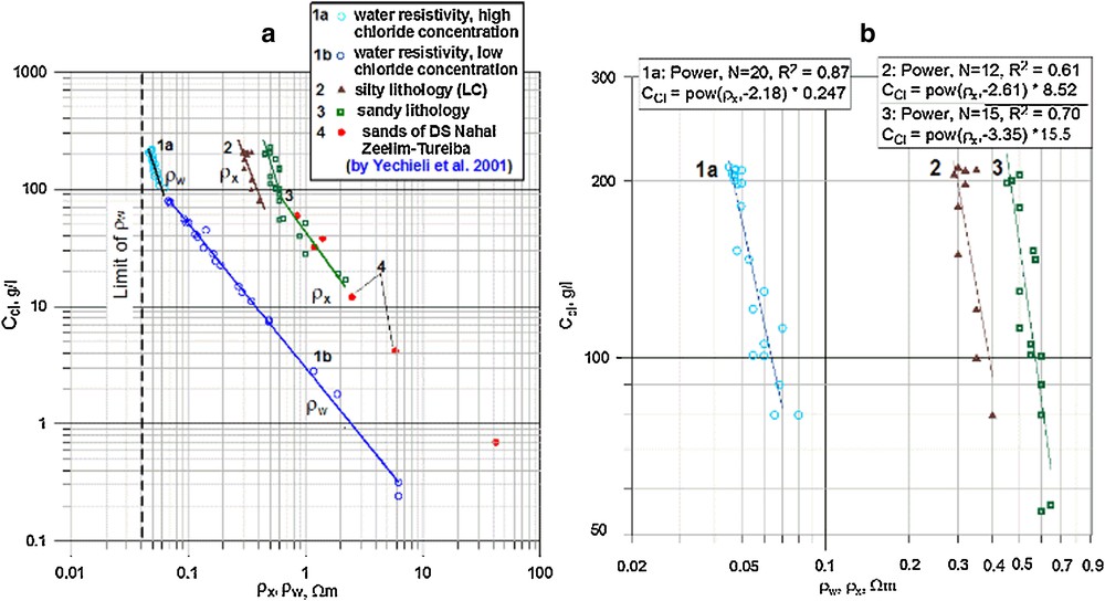
Various inter-relations between chloride concentration and resistivity: (a) all data; (b) high chloride concentration (new) data. Curves 1a and b represent high and low chloride concentrations in pore water (fluid) respectively vs. water resistivity þw based on GSI data, Yechieli et al., 2004; (2) chloride concentration vs. bulk resistivity Þx in lime carbonate sediments; (3) the same in saturated sandy sediments; (4) the same in sandy sediments of Nahal-Zeelim–Tureiba, after Yechieli et al. (2001).
Eqs. (2a) and (2b) allows the estimation of the chloride concentration of DS aquifers using groundwater resistivity ρw in boreholes.
The reason of nonlinearity of graph 1 as a function of salinity in the log–log coordinates is explained by Serra (1984, p. 9, fig. 1) as follows. At low salt concentrations, resistivity decreases (conductivity increases) as NaCl concentration increases up to a certain maximum, beyond which undissolved and therefore non-conducting salts impede the passage of current-carrying ions. A similar explanation was suggested by Keller and Frischknecht (1966). Therefore, we consider 214 gchloride/l (e.g., 258 g/l NaCl or TDS = 320 g/l) as the upper limit suitable for chloride concentration determination using electric conductivity (resistivity). This explains the two branches of Eqs. (2a) and (2b) characterized by different slopes in log–log coordinates.
5.4 Bulk soil resistivity–salinity relationships
Various relationships between chloride concentration and resistivity ρx are presented in Fig. 1a.
In Fig. 1a and b, the data plot 2 (triangles) presents chloride concentrations for sediments of lime carbonate vs. TEM-derived bulk resistivity. This group comprises boreholes Mn-1, Mn-2, Mn-4, Nz-1–NZ-9, HS-2. The TEM-derived bulk resistivity for lime carbonates is 0.3–0.45 Ω·m.
| (3) |
Data plots 3 (squares) correspond to sandy-gravel sediments in the relatively deep part of boreholes (at a late time of the transient), saturated by Dead Sea diluted brine with Cl concentration between 4.2 and 215 g/l. These sandy-gravel sediments have a resistivity ρx in the range of 0.45–5.8 Ω·m.
For high chloride concentrations
| (4a) |
For low chloride concentration
| (4b) |
These data have been added following the measurements of Yechieli et al. (2001) (solid circles–4) obtained along the DS (Nahal-Zeelim–Tureiba profile).
5.5 Bulk soil resistivity–water resistivity relationships: Archie's equation
The relationship between bulk resistivity ρx and water resistivity ρw is presented in log–log coordinates in Fig. S5.
The graph for sandy-gravel sediments allows fitting ρx and ρw data to Archie's equation for sediments with an effective porosity φe = 0.32
| (5) |
| (6) |
The Eq. (5) is similar to Archie's equation (see Kafri and Goldman, 2005), which is fitted to that of sandy-gravel sediments with effective porosity in the range of 0.25–0.30 (Ezersky et al., 2011). For comparison, Stephens et al. (1998) estimate the effective porosity range of sands at 0.24–0.32, whereas silt (very small like clay particles) has an effective porosity value of 0.44. The parameters of Archie's law for sand are a = 1.0 and m = 1.95, to be compared with 0.81 and 2 for Dead Sea sands, respectively (Kafri and Goldman, 2005).
5.6 Analysis of resistivity–salinity relationships
We have calculated curves of Ccl versus ρx based on Eqs. (4a) and (4b) for different porosities of sandy sediments. The calculations were performed in the following order: (1) the chloride concentration Ccl was selected in a wide range of values (1.5–200 g/l); (2) the water resistivity ρw was calculated from Ccl using Eqs. (2a) and (2b); (3) the bulk resistivity ρx was calculated using Eq. (5), keeping porosity fixed; (4) the calculation was repeated for another porosity value.
The calibration results are summarized in Supplementary Table S1 as follows:
- • the measured chloride concentrations CCIM are between 4.2 and 230 g/l (2–89% of saturation) in sandy-gravel sediments and between 187 and 245,5 g/l (71–95% of saturation) in lime carbonates;
- • the groundwater resistivity ρw has been measured either in boreholes or calculated using Eqs. (2a) and (2b). the groundwater resistivity varies between 0.045 and 0.247 Ω·m within the studied boreholes, expanding to 0.765 Ω·m within the boreholes of Yechieli et al. (2001);
- • the typical bulk resistivity value in lime carbonates, varies mainly between 0.25 and 0.35 Ω·m (generally, ρx < 0.4 Ω·m) in the DS coastal area, whereas gravel and sandy sediments are characterized by a resistivity ρx between 0.45 and 2.5 Ω·m (generally, 0.5–1.0 Ω·m). The results of Yechieli et al. (2001) expand this range to 5.8 Ω·m measured in boreholes located 3–5 km away from the Dead Sea shoreline. Thus, separated resistivity ranges allow distinguishing lime carbonate and sandy sediments saturated with DS brine based on resistivity values. The 0.4–0.45 Ω·m boundary looks a bit fuzzy. After our estimation from the data, some uncertainty of ±0.1 Ω·m can exist around 0.4 Ω·m. However, the methodology used for resistivity mapping through the investigation areas implemented by us on the basis of the antijamming TEM FAST system implies that numerous (2–4) measurements are needed at the same station, with a subsequent set of measurements at adjacent stations located 30–50 m apart.
Taking into account (1) that the lateral variation of salinity is slow through the area (Yechieli et al., 2001) and (2) that TEM averages the resistivity through the square of the effective ring (McNeill, 1980a), the diameter of which is 40-m at a 40-m depth in the DS coastal area. We can therefore consider the conditions of our measurements as 1-D. Then, making numerous measurements at the point and in its vicinity allows a statistically significant result, which roughly classifies the lithology based on bulk resistivity.
The relationships between ρx and ρw constitute the formation factor F that is stable enough in the range of resistivity measured in DS aquifers. As seen from Supplementary Table S1, the formation factor of sandy-gravel sediments and lime carbonates is, respectively:
| (7) |
| (8) |
The values of φe and ρw are also calculated using the relationships obtained above.
The effective porosity φe has been calculated using the formula derived from Archie's equations for sands Eq. (5) and for lime carbonates Eq. (6):
| (9) |
| (10) |
These equations allow the comparison of TEM based porosity values from 28 boreholes with those determined by geotechnical methods. Based on the results of Supplementary Table S1, one can conclude that the average effective porosity of sandy sediments calculated from Archie's law is φe = 0.32 ± 0.03, which is less than the total porosity φt = 0.4 measured in the laboratory. The average effective porosity of lime carbonates is φe = 0.44 ± 0.02, which is less than the total porosity of lime carbonate φt = 0.50 measured in laboratory. These results correlate well with hydrogeological data (Gibb et al., 1984; Stephens et al., 1998).
5.7 Constructing a salinity map based on bulk resistivity
5.7.1 New approach in the resistivity mapping of the DS aquifers
We have suggested a new approach based on the separate processing of TEM data through salt and the aquifer (Levi et al., 2011). The first stage is the delineation of the salt layer, which is an essential part of Dead Sea shores conditions. The salt layer inserts a significant heterogeneity of seismic velocities and electrical resistivity values to the investigated subsurface. Therefore, after locating the salt layer edge using the seismic refraction method (Ezersky, 2006), we can separate the area into two quasi-homogeneous sites of investigation: (1) “no salt” area located west of the salt edge, where the measured resistivity is influenced by groundwater salinity; and (2) “salt” area east of the salt edge, where the measured resistivity is affected by salt porosity at a constant water resistivity value. In addition, it allows avoiding 3D effects possible in the vicinity of the karstified salt. Note that in areas where the subsurface is composed of quasi-homogeneous sediments, seismic surveys will not be needed.
5.7.2 Parameters used for resistivity map constructing
In most places, we do not know ρw and Ccl in situ. Knowing ρx and the lithology, we can calculate directly the chloride concentration Ccl using Eq. (3) for lime carbonates or Eqs. (4a) and (4b) for sandy-gravel sediments. Where we have a borehole, we can evaluate groundwater salinity using resistivity (conductivity) logging within the borehole using Eqs. (2a) and (2b). It allows us to avoid both TEM measurements and laboratory analysis of groundwater samples.
Mutual relationships between ρx and ρw are given by Eqs. (5) and (6) for sands and lime carbonates, respectively. Eqs. (7) and (8) may also be used in the latter case.
An example of the resistivity versus depth functions in Supplementary Fig. S6 shows the parameters used for constructing a resistivity map.
The sounding carried out at the TEM-1 station (Supplementary Fig. S6a) is compared with the lithological and hydrological columns of boreholes Mn-1 (Supplementary Fig. S6b); similarly, the graph giving inverse resistivity versus depth at the TEM-2 station (Supplementary Fig. S6c) is compared with the lithological and hydrological columns of borehole Mn-2 (Supplementary Fig. S6d). Both boreholes are located along the line 2WE in Fig. 2a. The boreholes are located in different lithology (Fig. S6b and d). The Mn-1 borehole crosses sandy-gravel lithology with minor lime carbonates, whereas Mn-2 borehole crosses lime carbonate lithology both above and below a salt layer. These lithological differences result in different TEM sounding results. For TEM-1 station, the average resistivity of the layer under the water table is 0.58 Ω·m at a depth range between 24 and 40 m (Fig. S6a). This resistivity value can be now used to characterize the aquifer. The corresponding water resistivity ρw from Eq. (6) is of 0.061 Ω·m. The chloride concentration Ccl calculated from Eq. (2a) is 109 g/l. Direct calculation of Ccl using Eq. (4a) gives an estimation at 104 g/l. Salinity measurements in boreholes carried out in 2005 (Supplementary Fig. S6b) show a chloride concentration of ∼110 g/l. The discrepancy between calculated and measured values of Ccl is ∼4.8%. Such uncertainty in the evaluation of water salinity means that groundwater contains 46–49% of the chloride saturation value and keeps a high potential to dissolve halite (up to ∼112 g/l). So it can be considered as a satisfactory result.
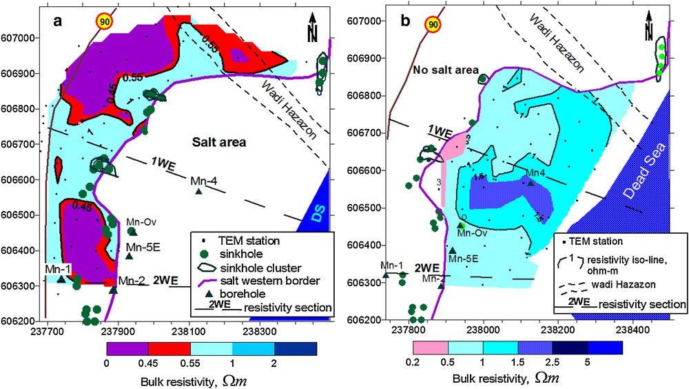
Two resistivity maps generated separately for aquifer (a) and salt layer (b), respectively, west and east of the salt layer border (thick solid line).
The TEM-2 resistivity-depth graph (Supplementary Fig. S6c) shows a very low resistivity of 0.25–0.3 Ω·m within lime carbonates saturated with Dead Sea brine (Supplementary Fig. S6d). The chloride concentration calculated using Eq. (3) is in the range of 240–198 g/l. The measured chloride concentration is 200.5 g/l. Note that the chloride concentration has been corrected with respect to the date of TEM measurements in accordance with monitoring data (Yechieli, 2007). These resistivity values and chloride concentrations are used for constructing resistivity and chloride concentration maps. The TEM FAST equipment enables to carry out numerous measurements both at the same station and in its vicinity.
5.7.3 Example of resistivity mapping of the Mineral Beach aquifer
The Mineral Beach area (see Fig. S2 for location) is mainly composed of sandy-gravel sediments. The geology of the site has been presented in a number of publications (e.g., Frumkin et al., 2011). The methodology includes fast spatial mapping of the bulk resistivity in both vertical and horizontal directions through the area, covering ∼1 km2. Two resistivity maps are shown in Fig. 2. Fig. 2a presents the lateral resistivity distribution in the “no salt area” (west of salt edge shown by a thick solid line) at the salt elevation. A resistivity map through the salt layer east of the salt edge is shown in Fig. 2b.
As an example, we construct a map of the calculated water salinity Ccl throughout the aquifer of the Mineral Beach area west of the salt edge (Fig. 3). The map is opposed to the resistivity map of the aquifer (Fig. 2a). Zones of high chloride concentration in Fig. 3 correspond to zones of low bulk resistivity in Fig. 2a. Moreover, zones of low chloride concentration correlate with the sinkhole clusters line along the salt edge.
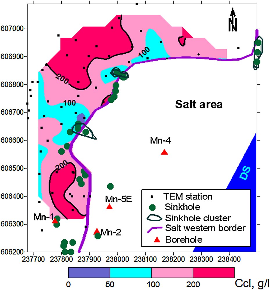
Evaluation of groundwater salinity through Mineral Beach area using resistivity distribution. The map of water salinity at the depth of the salt layer is based on measured Þx values and calculated values of chloride concentration after Eqs. (3), (4a), and (4b).
Borehole Mn-1 at the southern part of the map has a chloride concentration of 110 g/l (Supplementary Fig. S6b).
The borehole is located at the border between two zones where the calculated chloride concentration is close to the value of 112 g/l.
Thus, borehole data can be used to test the reliability of the salinity map. Based on the salinity map, one can suggest that brackish groundwater came from the nearby marginal fault west of the salt edge (central part of the map).
6 Discussion
6.1 Lithology as factors affecting salinity determination
As it was mentioned above, Archie's Law is generally an appropriate resistivity estimator in a so-called “clean sand” (clay free) environment. The clay content results in significant surface conductivity. With increasing the clay content, the soil becomes “shaly sand”, and corrections must be applied to Archie's law (Schoen, 1996). Thus, bulk electrical conductivity (resistivity) depends also on the clay content, among other factors. One can see in Supplementary Table S1 (column 4) that lime carbonate sediments show bulk resistivity lower than 0.4 Ω·m, whereas sandy sediments have a resistivity value higher than 0.4 Ω·m. The calculated effective porosity of sandy sediments based on these resistivity values is 0.27–0.35 (average value of 0.32), i.e. is in the range of reported by other researchers (Kafri and Goldman, 2005; Stephens et al., 1998). Surprisingly, the effective porosity of lime carbonate (also referred to as DS mud), calculated using Archie's Eqs. (6) and (10), ranges between 0.42 and 0.46 (average value: 0.44), which is within the limits presented by Stephens et al. (1998) for the effective porosity of silt. One can presume that the CEC effect does not (or very slightly) affect the resistivity values of lime carbonate. The slight influence of the CEC effect would be explained in two ways. At first, lime carbonate either does not contain or contain negligible content of kaolinitic clay (∼2.35 mequiv/100 g and low total specific surface area), resulting in low CEC values (Khlaifat et al., 2010). This is in agreement with the composition of the fine detritus material in the DS basin (Haliva-Cohen et al., 2012). In other words, lime carbonate (DS mud), which in the past was considered as DS clay (Arkin and Gilat, 2000), in reality exposes properties of silt rather than of clay. It is supported also by the conclusion of Frydman et al. (2008) on the absence of cohesion in lime carbonate and on its mechanical behavior, which is similar to sand. The other explanation of the low CEC effect is the very high-salinity of the pore water. Shevnin et al. (2006), using petro-physical modeling (see Supplementary Fig. S7), have shown that an increase in water salinity (up to 100 gsalt/l) results in a decrease of the influence of the clay content on bulk resistivity. For instance, at a salinity of 1 g/l, the resistivity of clean sand and of sand mixed with 70% clay is 50 and 2.5 Ω·m, respectively (20-fold difference). At a salinity of 100 g/l, the values are 1 Ω·m and 0.5 Ω·m respectively (2-fold difference only). We can reasonably presume that this difference will be lower at higher (up to 240 g/l) levels of salinity.
We assume that both factors are present and act simultaneously, resulting in low CEC effect in the DS lime carbonates.
It means that one can calculate porosity values in both sandy sediments and lime carbonates (DS mud) using the TEM method. Porosity, in turn, is an important parameter for the evaluation of hydrogeological aquifer properties, such as storativity (Kafri and Goldman, 2005).
6.2 Comparison of resistivity–salinity relationships obtained by various researchers in Israel
We compare the resistivity–salinity relationships obtained by various researchers in Israel (Fig. S8). One can see that the data of this study (triangles) agree well with the relationships obtained within similar Quaternary sandy-gravel sediments along the Dead Sea shore (solid circles in Fig. S8) and the Mediterranean coastal areas in Israel (Kafri and Goldman, 2006).
At the same time, the relationship obtained by Levi et al. (2008) shows resistivity values that are approximately 2.5–3.0 times higher than our results at the same salinity (crosses).
The relationships presented in Fig. S8 at first confirm the conclusions of Kafri and Goldman (2006) that the correlation between TEM bulk resistivity and groundwater salinity is excellent for high-salinity brines exceeding 10 g/l of chloride, but greatly deteriorates with decreasing salinity associated with brackish and fresh waters. It corresponds well to the conclusion of Yechieli et al. (2001, p. 373) that in cases of high groundwater salinity measured within boreholes (decades–hundreds of gchloride/l), salinity is the main factor governing TEM resistivity, regardless of differences in other factors such as lithology (i.e. composition, texture, grain size, etc.) and porosity. Our study supports this conclusion for a range of very low resistivity values lower than 1 Ω·m. It can be seen from Fig. S8 (triangles) that there is practically no scatter in this resistivity range. It is seen also from the graph in Fig. S5. On the other hand, deep aquifers are strongly scattered (Levi et al., 2008).
It can be seen also that the slopes of the Ccl vs. ρx plots in the range of low (0.45–2 Ω·m) and high resistivity (> 2 Ω·m) are different (triangles and solid circles, respectively, in Fig. S8).
This conclusion is especially valid in Quaternary sediments located at a depth range of 25–60 m, whose pores are filled with DS brine (150–200 gchloride/l) and saline water (10–150 gchloride/l), corresponding to a resistivity range between 0.2 and 2.0 Ω·m (triangles in Fig. S8, this study). Similar results were reported by Kafri and Goldman (2006) who studied relationships in similar sediments at a depth range of 95–200 m along the Mediterranean coast of Israel (circles in Fig. S8). At the same time, the relationship presented by Levi et al. (2008) (crosses in Fig. S8) were obtained in more ancient carbonate rocks and sandstones at a depth range of 220–2000 m. In this case, porosity should strongly affect bulk resistivity. The resistivity–salinity relationships obtained in our study and by Kafri and Goldman (2006) are well fitted to the 0.40 porosity graph, whereas the relationship derived by Levi et al. (2008) agrees with the 0.20–0.30 effective porosity range.
7 Conclusions
Twenty-eight TEM soundings along the Dead Sea (DS) coastal area were carried out close to observation boreholes to generate quantitative relationships between bulk resistivity (ρx), water resistivity (ρw), and chloride concentration (Ccl) in a resistivity range below 1.0 Ω·m in order to evaluate the aquifer salinity in in situ conditions. The main findings of the study can be formulated as follows:
- • we have studied aquifers saturated with high-salinity brine characterized by resistivity values between 0.2 and 1.0 Ω·m along the DS coastal areas using the TEM FAST methodology;
- • in the DS coastal areas, the formation factor F = ρx/ρw throughout the bulk resistivity range ρx < 1.0 Ω·m is practically constant and equal to 9.9 ± 1.3 for sandy-gravel sediments and 5.8 ± 0.7 for lime carbonate (DS mud);
- • quantitative relationships between bulk resistivity ρx, water resistivity ρw, and chloride concentration were derived. These relationships enable calculating chloride concentrations Ccl based on bulk resistivity measured from the surface, using TEM or on borehole measurements of water resistivity (conductivity);
- • average effective porosity values φe of sandy-gravel sediments and silty lime carbonates (DS mud) estimated by the TEM method are 0.32 and 0.44, respectively. The total porosity values φt measured in the laboratory and in in situ conditions are 0.40 and 0.50, respectively;
- • Archie's Law for DS sediments has been fitted to the above relationship using φe porosity measurements. It enables to use TEM bulk resistivity to evaluate hydrogeological parameters such as yield, storativity, etc.;
- • lime carbonate demonstrates the same properties of cohesionless sediments and does not exhibit the Cation Exchange Capacity (CEC) effect. This allows the use of Archie's Law in lime carbonate;
- • it was known earlier that bulk resistivity values lower than 1 Ω·m unambiguously define the presence of DS brine in the pores of alluvial sediments without respect to lithology. However, it follows from this study that a DS aquifer with bulk resistivity in the range of 0.55–1.0 Ω·m contains pore-brine with 110–50 gchloride/l (50–22% of the saturation value, respectively), i.e. it keeps a potential to dissolve up to 114–174 gsalt/l and therefore it is aggressive with respect to buried salt layers;
- • the calibration near boreholes suggests that sedimentary rocks with high silt content saturated with Dead Sea brine are characterized by resistivity values ρx < 0.4 Ω·m (generally, 0.2–0.3 Ω·m), whereas sandy material saturated with Dead Sea brine has a resistivity of ρx > 0.4 Ω·m. This allows identification of silt saturated with the Dead Sea brine using only TEM measurements.
We suggest that salinity–resistivity relationships derived in this study are strictly valid, not only for Israel, but also for other areas of the world in similar conditions (salt/arid climate, etc.).
Acknowledgments
This work was made possible through support provided by the U.S. Agency for International Development, under terms of Award No. M27-050. We are grateful to Y. Yechieli for providing hydrological materials regarding the investigated areas. We thank Tamar Regional Council and National Roads Company of Israel (MAAZ) for numerous drilling data. We are grateful also to reviewers M. Descloitres and K. Chalikakis for attentive reading of the manuscript and useful comments.