

1 Introduction
The Earth's rotation axis, close to the polar inertia axis, presents, with respect to the mantle, variations at different time scales, from daily to secular. The trace of the rotation axis at the surface of the Earth is generally considered to be the sum of three components: the annual wobble, a forced oscillation due to an atmospheric excitation, the Chandler wobble, a free oscillation with a period of 435 days, whose maintaining mechanism is not yet fully understood, and the so-called drift of the mean pole (e.g., Chandler, 1891a; Chandler, 1891b; Gibert and Le Mouël, 2008; Hulot et al., 1996; Lambeck, 2005). In the present paper, we will add a fourth periodic component, that we attribute to solar activity.
In 1967, Karklin (1967) analyzed the International Latitude Service data from 1900 through 1959, and found variations in the amplitude of both the Chandler and the annual oscillations with decadal periods (e.g., 10.3, 12.3, 17.7 years for Chandler) and amplitudes of a few 10−2 arcsec (1 arcsec ∼ 4.85·10−6 rad) that he attributed to Solar activity. Jady (1970) estimated the torque exerted by the solar wind on the Earth's magnetic dipole, using a simplified model of magnetosphere (a thin planar, perfectly conducting sheet). He found that the magnitude of the torque (1.1·1016 J) was smaller than that required to account for the change in the length of the day (l.o.d), but comparable to the lunar tidal torque (2.7 1016 joules). It seems that this mechanism has not been considered further since then.
2 The SSA analysis of the series of pole positions
We will use here the series of pole positions produced and issued by the International Earth Rotation Service (IERS; web site: http://www.iers.org/IERS/EN/Science/EarthRotation/EarthRotation.html) in the form of a yearly report (EOPC01); the 2015 EOPC01 report is considered. mx and my are the components of the pole position in a tangent plane Oxy at the north pole (or in the equatorial plane). O is a conventional origin, the axis Ox is in the Greenwich meridian, the axis Oy is in the 90°E meridian; the sampling interval is 0.6 month. Data mx and my cover a period from 1900 to 2015 (see Fig. 1); they will be counted in rad·s−1, like the Earth's spin itself. We analyze those series through singular spectrum analysis SSA (Vautard and Ghil, 1989) (see Appendix). The components of the pole motion extracted by SSA are ranked according to their “importance” (that is their amplitude, in a broad sense): first the annual oscillation (SSA component 1, prograde and retrograde), then the Chandler term (SSA component 2, wobble), then with the same “importance” the trend that can be seen as the component of the mean pole drift (SSA component 3). Two other components, with an “importance” two times smaller, are identified mainly along the axis my (they are smaller, by about one order of magnitude, along the axis mx):
- • an oscillating component with segments containing quasi-pure sinusoidal variations with a 11-year period and a characteristic amplitude of ∼0.5·10−12 rad·s−1, which we note and a central segment presenting a sine variation with a 22-year period; the amplitude of the latter component is ∼1.4·10−12 rad·s−1; we note it (SSA component 4, see Fig. 2). During the reconstruction process of each component obtained with SSA, we regroup them according to the magnitude of their associated eigenvalues (see Appendix). That is why, in this specific case, an oscillating variation composed of two distinct periods is reconstructed;
- • a component with a smaller characteristic amplitude (∼4·10−13 rad·s−1), displaying 5.5-year modulated periodic sine oscillations (SSA component 5, see Fig. 3).
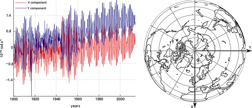
Polar motion data series (EOPC01) provided by the International Earth Rotation Service. The X and Y components, mx, my, correspond to the red and blue lines respectively. mx and my are given in rad·s−1.
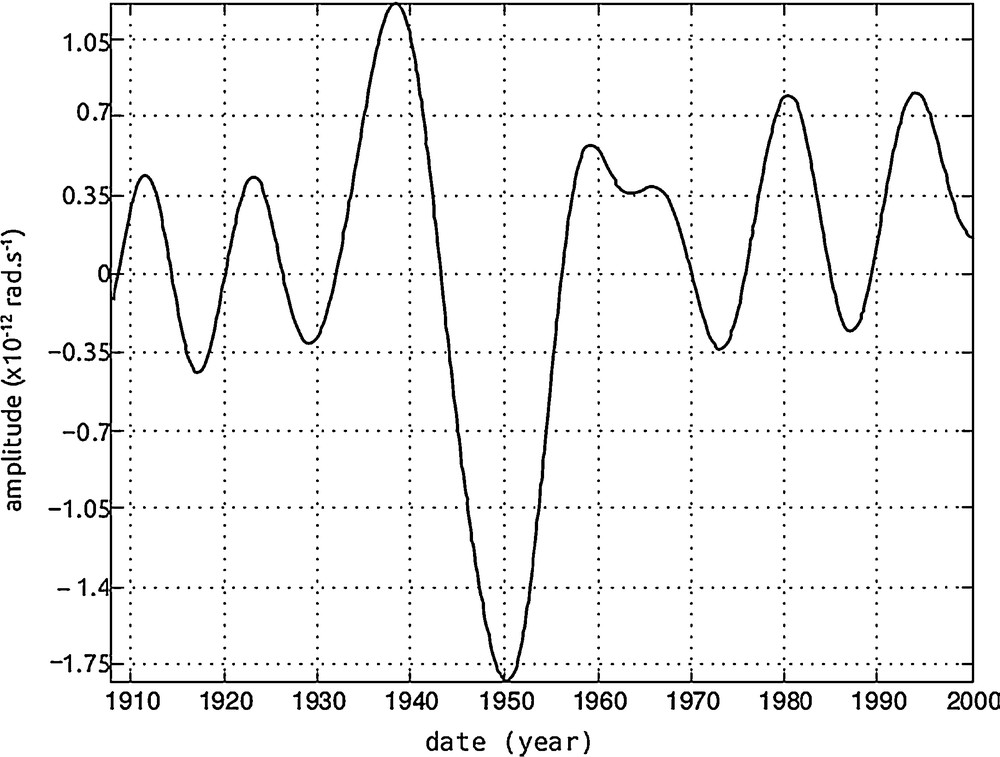
Oscillating signal extracted, using SSA, from my: “component 4” displays quasi-pure oscillations with a 11-yr period, and, in the central part, one oscillation with a 22-yr period.
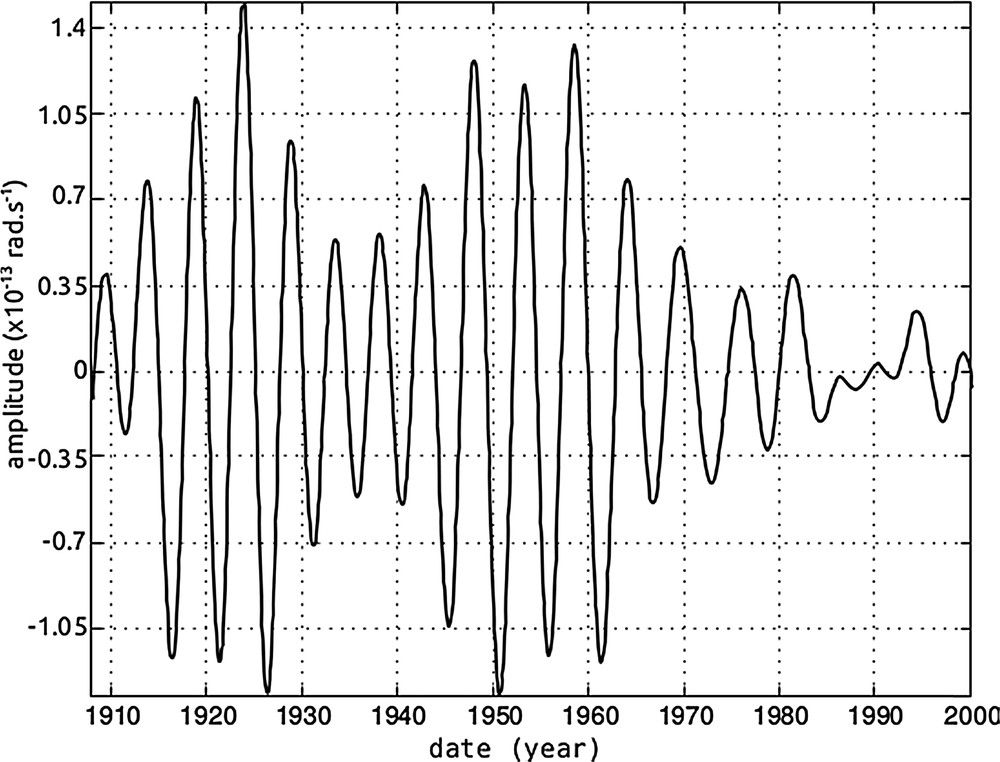
Oscillating signal extracted, using SSA, from my: “component 5” displays quasi-pure oscillations with a 5.5-yr period.
3 A tentative interpretation
We consider here that the periodic oscillations (with periods 22 years, 11 years and 5.5 years) detected in the series of pole positions are manifestations of solar activity for lack of any reasonable alternative. In this short note – devoted essentially to unveiling these periodicities – we do not attempt to propose a full explanation of their presence in the rotation pole series, but only to evoke some elements of a possible mechanism. First, a direct electromagnetic torque exerted by the solar wind on the Earth's main magnetic field, i.e. on the conducting core (the dipole according to Jady, 1970), transmitted to the mantle through some kind of core–mantle coupling (e.g., Jackson, 1997; Jault and Le Mouël, 1991) could be envisioned. We have mentioned in the introduction the first attempt made by Jady, concerning l.o.d., but this process appears to lead to insufficient torques. A second mechanism, which we now elaborate somewhat further, involves an action of solar activity on the atmosphere, resulting in flows, or winds, and a transfer of angular momentum from the atmosphere to the mantle.
3.1 Schematic atmospheric flows
Since the vertical component of large scale winds in the atmosphere is small compared with the horizontal one, and the thickness of the different layers is small compared with the Earth's radius r, we assume velocities to be purely horizontal and adopt a thin layer approximation (Chedin et al., 1982). A layer of thickness h, between radii a and b, is replaced by a surface layer of density (kg·m−2). The horizontal divergence-free velocity field can be represented by an expansion in elementary toroidal vectors,
| (1) |
| (2) |
| (3) |
is the unit vector of Oy axis; a similar expression holds for . It is easily seen that only the elementary velocity vector,
| (4) |
contributes to the angular momentum of around Oy. We will write this term in the equivalent form,
| (5) |
3.2 Estimates of atmospheric winds
Applying SSA analysis (see Appendix) to the evolution of my, the equatorial components of the mantle rotation axis in the 90° east meridian, we have found three periodic components with periods 11 years, 22 years, and 5.5 years, with amplitudes directly measurable in Figs. 2 and 3 (in 10−12 rad s−1). These components are about one order of magnitude smaller for mx. Multiplying these amplitudes by the equatorial inertia momentum of the mantle (A = 8·1037 kg m2), we obtain the amplitudes of the corresponding periodic variations of the equatorial angular momenta of the mantle,
| (6a) |
The same computations give for the x component:
| (6b) |
Let us come back to our simplified flow in the atmosphere. We consider that the mantle-atmosphere system is isolated (neglecting the changes in the small angular momentum of the core); the changes in the equatorial angular momentum of the mantle are attributed to exchanges of momentum between the mantle and an atmospheric layer to which solar activity communicates motions with solar periods and the geometry given by formula (5). And, aiming only at orders of magnitude, we simply write that changes in angular momenta of the (schematic) atmospheric flows, balance the corresponding mantle angular momentum periodic variations (the same for the smaller x components). Now, the expressions of the σ are (taking e.g., and the 11-yr period),
| (7) |
Equaling (and dropping the exponential factor), we obtain:
| (8) |
The numerical value of Amy is given by (6). The same expressions hold for the other lines and the x components. Of course, the angular velocity ω cannot be found independently of H.
4 Discussion
Wind velocities in the atmosphere have long been measured (e.g., Drob et al., 2015; Pichugina et al., 2012; Talaat and Lieberman, 2010). Zonal wind velocities can reach 60 ms−1 (Fleming et al., 1990; Gross et al., 2005; Salby and Callaghan, 2000). They do not contribute to the components. Meridional flows do contribute, but they are much smaller, of the order of a few ms−1 (Gudiksen et al., 1968; Nastrom et al., 1982; Oort and Rasmusson, 1970). Let us consider the periodic flows computed in Section 3, in the case when the layer concerned by the flow is the troposphere. Then H ∼ 104 kg m−2, and from formula (8), we get:
| (9) |
In the same way, .
In terms of linear velocities uH, the orders of magnitude, obtained simply by multiplying ω by r = 6.5 106 m, are
| (10) |
The periodic flows computed in Section 3 in the frame of our schematic model take the form of rigid equatorial rotations, a kind of image of the equatorial rotations of the solid mantle. They have magnitudes compatible with measured meridional flows in the troposphere. Such flows, if present, might be difficult to evidence directly, taking into account, in particular, the long (solar) periods involved. In fact, as noticed in Le Mouël et al. (2010), the solid mantle would play the role of an integrator, revealing these periodic large-scale motion variations (a velocity field is transformed into a rotation vector). We can call also upon stratospheric winds. Indeed, up to now, we have skipped a major step of the proposed process, the means by which solar activity can affect circulation in the atmosphere. We recall that the view according to which the solar cycle can affect the climate is not favorably received, for the main reason that during a solar cycle total solar irradiance varies by only 10−3. But, first, the different wavelengths are not modulated by the same factor during a cycle. Second, electromagnetic irradiance is not the only acting power to take into consideration; one may call upon solar wind, galactic cosmic rays, and induced effects on ionospheric electric currents, acting in particular on clouds (Gray et al., 2010). We elaborate only briefly on the mechanism we invoke above, which requires interactions, couplings, between different layers of the atmosphere. Variations in solar UV radiation influence directly the ionosphere; links between processes having their seats in the ionosphere and in the stratosphere have been “demonstrated” (Rishbeth, 2006). “Transfers of energy and momentum happen” (Forbes, 2000; Gray et al., 2010). In fact, much interest is presently devoted to the coupling between the stratosphere and the ionosphere up to altitudes of several hundred kilometers. Coupling between stratosphere and ionosphere has been evidenced from a number of different sources (e.g., Baldwin and Dunkerton, 2001, Goncharenko et al., 2010); Kuroda and Kodera (2005), in a long paper devoted to solar influence on climate, write “Understanding the physical mechanisms connecting the lower and upper atmosphere will be an essential part of future models...” and “Considering the upper atmosphere as a part of a complex and evolving Earth system is a necessary step for further advances...”. Our findings imply some form of coupling between the solid Earth and the atmosphere. Such coupling is established through the observations of a good correlation between some l.o.d. variations and the angular momentum of the atmosphere for periods up to a few years. Indeed, some l.o.d. variations are attributed to exchanges of angular momentum between the mantle and the atmosphere (e.g., in Lambeck, 2005).
5 Conclusion
We have found evidence of periodic solar components in the mantle pole position time series (with periods of 5.5 years, 11 years and 22 years): oscillations occur mainly along the equatorial 90° east meridian, with an amplitude of 0.5 10−12 rad s−1 for the 11 year-oscillations, of 1.5 10−13 rad s−1 for the 5.5-year oscillation, and of 2 10−12 rad s−1 for the 22-year oscillations. We argue that this oscillation (wobble) of the solid mantle can result from an exchange of angular momentum with an equatorial flow in the terrestrial atmosphere, an image of mantle libration. With this hypothesis, we obtain an order of magnitude of 1 m s−1 for the flows (wind velocities), compatible with meridional velocities measured in the atmosphere. These solar-generated atmospheric winds would not be small.
Acknowledgements
The authors and the editor-in-chief wish to thank Drs. Kurt Lambeck and Dominique Jault for their reviews and comments of this paper at both early and quasi-final stages. IPGP Contribution No. 3857.
Appendix A Singular spectrum analysis
A thorough account of singular spectrum analysis (SSA) is given for instance in Vautard and Ghil (1989) and Vautard et al. (1992). SSA is a powerful, non-parametric, time series analysis tool that relies on the Karhunen–Love spectral decomposition (Kittler and Young, 1973). We summarize it here for the reader who would not be familiar with the method.
Consider the real-valued time series x = {xn: n = 1,…,N}; SSA decomposes vector x into a sum of physical components that may be subsequently identified as trends and quasi-periodic oscillations. The starting point is to embed x into an L-dimensional vector space, by using lagged copies of x L that are K = N–L + 1 long. In other words, form the following “trajectory” (Hankel) matrix X:
The next step consists in performing the singular value decomposition (Golub and Kahan, 1965) of the trajectory matrix XXT; we obtain a collection of eigen-triplets {λi: i = 1;…; L} of XXT, which are ranked in the decreasing order of magnitude (λ1 ≥ λ2 ≥···≥ λL ≥ 0). The eigen-triplets are linked by Vi = XTUi/√λi. Once this decomposition is made, the last stage consists in the construction of groups of components. Each group is a subset of matrices Xi; let I = {i1,…,ip},be a group of indices {i1,…,ip}, the corresponding matrix Xl = Xi1 +···+Xip, thus the matrix becomes X = Xl1 +···+Xld. The choice of the indices in each group is done empirically; for that, we may find it interesting to group the eigen-triplets that have common eigenvalues.