

1 Introduction
Dobson (1999) has proposed the recognition of a vast geographical Earth feature – named aquaterra – encompassing the lands that have been inundated and exposed during the last 120,000 years in consequence of the waxing and waning of the continental ice sheets. The study of the extent and chronology of aquaterra impacts various disciplines of Earth sciences and has also a number of cultural aspects. In particular, knowledge of the detailed evolution of aquaterra could shed light on the human history and on the occupation of landmasses in the past (Flemming, 1985), also providing clues on the pathways of diffusion of material culture (Cavalli-Sforza et al., 1993). Recently, Dobson (2014) has refined the description of aquaterra. Furthermore, he has also outlined possible strategies for the exploration of aquaterra, which would demand a major collaboration between geographers and oceanographers for its exploration.
Before a systematic exploration of aquaterra may become possible, global models of Glacial Isostatic Adjustment (GIA, see Spada, 2017, for a review) can be used to constrain its evolution in space and time. Since the seminal work of Peltier (1994), methods for the reconstruction of the ice age paleotopography have become available, based on the solution of the so-called “Sea Level Equation” (SLE) first introduced by Farrell and Clark (1976). The SLE, which describes the time evolution of sea level in response to the melting of the late-Pleistocene ice sheets, can be solved to predict the changing shape of the shorelines, employing suitable high-resolution numerical methods (see Spada and Stocchi, 2007; Spada et al., 2012). In GIA models, the history of sea-level change is determined by taking the variations of the equipotential geoid surface into account and reconstructing the paleotopography iteratively. Earth rotation effects are also accounted for. For these reasons, GIA models are “gravitationally” and “topographically self-consistent” (Peltier, 1994). Isostatic effects are of interest in the present context, since Dobson (2014), as a first approximation, did not take them into account. Thus, so far, the spatial and temporal extent of aquaterra has been defined with the implicit assumption of eustatic (i.e. spatially uniform) sea-level variations.
In this note, following the hint of Dobson (2014), we aim at refining the description of aquaterra by means of up-to-date GIA modelling. In particular, we shall consider the role of isostasy on the submergence of aquaterra since the Last Glacial Maximum (LGM, ∼ 21,000 years ago). During this period, major cultural innovations (see Fig. 3 in Dobson, 2014) and human dispersal occurred (Flemming, 1985; Lahr and Foley, 2004). Furthermore, after LGM existing GIA models define the history of the ice sheets to a sufficient level of detail. By a global analysis and some regional examples, we shall show that dynamic (i.e. non-eustatic) processes associated with isostatic deformation, mantle rheology, Earth rotational fluctuations and time variations of topography have affected significantly the extent and evolution of aquaterra.
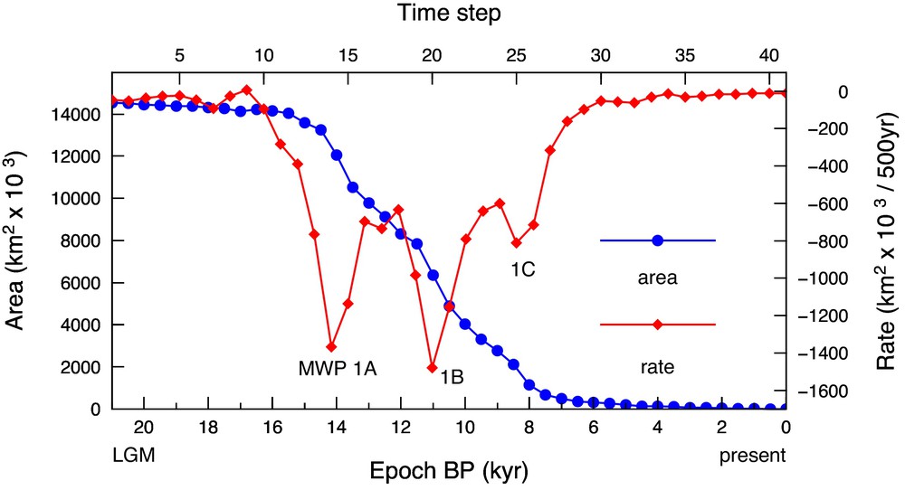
History of the exposed area of aquaterra (blue) and of its rate of change (red) from the LGM to present, according to the dynamic aquaterra model. The times of occurrence of the three meltwater pulses MWP-1A, 1B and 1C are also shown.
2 Methods
We follow the GIA theory illustrated by Mitrovica and Milne (2003), which generalises the original formulation of the SLE due to Farrell and Clark (1976). The SLE is obtained by imposing mass conservation within the system composed by the Solid Earth, the oceans and the ice sheets, keeping at the same time the sea surface equipotential. The resulting sea-level variations are not uniform across the oceans because of the effects of gravity and deformation, which are delayed as a consequence of the viscoelastic response of the mantle (e.g., Spada, 2017). In the generalised formulation, the SLE accounts for the horizontal migration of shorelines, for the presence of marine-based ice (distinguishing between grounded and floating conditions) and for the effects of rotational feedbacks on sea-level change (Milne and Mitrovica, 1998). The SLE is solved numerically by an improved version of program SELEN (Spada and Stocchi, 2007; Spada et al., 2012), employing an icosahedron-based equal-area grid (Tegmark, 1996) with a spacing of ∼ 20 km, sufficient to describe the isostatic effects on the global distribution of aquaterra in detail. The length of the integration time step is 0.5 kyr.
In this study, following the suggestion by Dobson (2014), we account for glacial isostasy adopting the global deglaciation chronology ICE-5G(VM2) of Peltier (2004) for the continental ice complexes. It assumes isostatic equilibrium before the LGM, and no deglaciation during the last 4 kyr. ICE-5G(VM2) is constrained to fit a global set of relative sea-level (RSL) data and represents a refinement of previous ICE-X models developed by W. R. Peltier (see, e.g., Peltier, 2004, and references therein). The ice thicknesses of continental ice sheets at the LGM and at present time according to ICE-5G(VM2) are shown in Fig. 1. In this work, we adopt a volume-average of the original multilayered viscosity profile VM2 (Peltier, 2004), with a viscosity of 2.7, 0.5, and 0.5 × 10²¹ Pa·s in the lower mantle, transition zone and shallow upper mantle, respectively. The thickness of the elastic lithosphere is 90 km. It is worth noting that GIA models are affected by some uncertainty, associated with limited knowledge about the melting history of the ice sheets and the rheology of the Earth. As a consequence, it should be taken into consideration that different GIA models can provide slightly different predictions for the history of sea-level change, which will also affect the features and evolution of acquaterra.
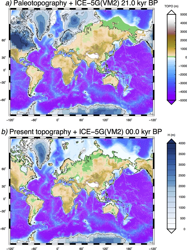
Paleo-topography al the LGM, reconstructed solving the SLE (a). The present-day topography, corresponding to ETOPO1, is shown in (b). The global ice thickness distribution according to the GIA model ICE-5G(VM2) is also shown.
Following Mitrovica and Milne (2003), paleobathymetry is reconstructed by performing two nested iterations of the SLE. In the internal iteration, the SLE is solved for a given a priori distribution of bathymetry; in the external one, the bathymetry is updated be means of the pattern of relative sea-level change obtained in the internal iteration. This procedure is performed adopting the “bedrock version” of the one arc-minute resolution ETOPO1 global relief (Amante and Eakins, 2009) as the present-day condition. The Earth's topographies at the LGM and at present time are shown in Fig. 1.
3 Results
We first consider the evolution of aquaterra from a global viewpoint; then we show results obtained for a few regional case studies.
3.1 A global view
A first guess of the global distribution of aquaterra since the LGM is shown in Fig. 2a, where blue pixels mark a grid cells belonging to aquaterra. To obtain this map, which is broadly in agreement with that in Dobson (2014), we have subtracted 127.3 m of water from the globally gridded ETOPO1 distribution, corresponding to the total equivalent sea-level rise since the LGM according to ice model ICE-5G(VM2). Hence, what we have obtained in this way is independent of the history and of the actual geographical distribution of past ice sheets, being determined by the present bathymetry and on the total volume of ice melt since the LGM. Such an approximation is equivalent to assume a spatially uniform (i.e. eustatic) sea-level rise across the ocean basins. Since eustasy implies the assumption of a rigid Earth and of negligible gravitational interactions between the solid Earth, the ice sheets and the oceans (see, e.g., Spada, 2017), the aquaterra map in Fig. 2a has a static rather that a dynamic character. According to the eustatic approximation, the area of aquaterra amounts to 22.5 × 10⁶ km2, i.e. 4.4% of the area of the Earth's surface. Note the limited development of aquaterra below 45° S, due to the relatively narrow and unusually deep Antarctic continental shelf (Padman et al., 2010). Some basic statistics about the spatial distribution of aquaterra are shown in Table 1. A prevalence of aquaterra in the northern hemisphere is also confirmed for the past 120,000 years (Zong, 2015).
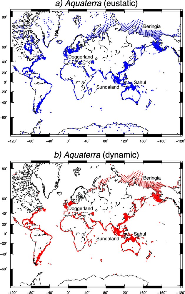
The spatial distribution of aquaterra according to the eustatic (a) and to the dynamic model (b). Major recognised land bridges, i.e. Beringia, Doggerland, Sundaland and Sahul, are also shown. Note that the Mercator projection exaggerates the polar region areas
Statistics of the spatial distribution of aquaterra across three latitudinal sectors, according to the dynamic and to the eustatic definition.
| Sector | Aquaterra (dynamic) area (km2) |
% | Aquaterra (eustatic) area (km2) |
% | Range of latitude (°) |
| North | 4,808,790 | 28 | 8,331,195 | 37 | φ ≥ + 45° |
| Centre | 11,873,805 | 69 | 12,176,880 | 54 | −45° ≤ φ ≤ + 45° |
| South | 491,655 | 3 | 1,946,415 | 9 | φ ≤ −45° |
| Total | 17,174,250 | 100 | 22,454,490 | 100 |
It is interesting to compare the static aquaterra distribution in Fig. 2a with that obtained when the GIA problem is solved consistently; this is shown in Fig. 2b by red pixels. Based on our paleotopographic reconstruction (two snapshots are shown in Fig. 1), these are the pixels that are currently submerged, but that have been emerged and ice-free at least during one time step (i.e. for 500 years) since the LGM. According to this dynamic definition (others are possible, indeed), aquaterra mostly occupies the continental shelf and, at mid and low latitudes, it contours most of the world's shorelines, in qualitative agreement with Dobson (2014) and with Fig. 2a. However, the introduction of isostatic effects has significant quantitative consequences. For example, the area of aquaterra is ∼ 17.2 × 10⁶ km2, which approximately corresponds to 3.4% of the area of the whole Earth's surface. This is a sizeable reduction (by ∼ 25%) with respect to the eustatic distribution of aquaterra. At high latitudes, the aquaterra distribution is quite complex and shows a major development in correspondence of the East Siberian Sea and Beringia. When the GIA problem is solved consistently, aquaterra disappears from part of the Hudson Bay, from the Canadian Arctic Archipelago, and from the Baltic Sea (compare with Fig. 2a). Some of the pixels belonging to these regions are now below sea level, but since the LGM they have never been emerged (nor ice-free) in consequence of the isostatic depression caused by the former ice sheets. It is worth noting that the distribution of aquaterra across Doggerland, located in the periphery of the previous Würm ice sheet, is affected by isostasy. The same occurs in the Baltic Sea region. The extension of aquaterra in Beringia appears to be less affected, since this region has been ice-free since the LGM and isostatic disequilibrium has been important. However, a more quantitative account of the dynamic effects acting across these regions requires the study of the sea-level curves from specific locations, which will be done in Section 3.2 below.
The blue curve in Fig. 3 shows the area of aquaterra since the LGM, obtained by the dynamic model. The plot provides insight into the time evolution of aquaterra, which can be broadly divided into three major phases, each with a duration of ∼ 7000 years. During the early and the late phases, the area has remained close to stationary, while during the central period the aquaterra has been subject to a major reduction until its substantial disappearance. In the central phase, however, the evolution of aquaterra has been quite complex, and characterised by intermittent variations in consequence of the pulses of ice-sheet meltwater that occurred within this time frame (Fairbanks, 1989; Fairbanks et al., 1992; Gornitz, 2013; Stanford et al., 2011). These can be better visualised by computing the time-derivative of the history of the aquaterra area (red curve), which is indeed marked by three minima corresponding to periods of enhanced loss of area, corresponding to Melt Water Pulses MWP-1A, 1B, and 1C (Blanchon, 2011; Gornitz, 2013). Although MWP-1A (between 14.3 and 12.8 ka BP) is of a multi-centennial to millennial nature, MWP-1B can be more appropriately described by a broad multi-millennial peak between 11.5 and 8.8 ka BP (Stanford et al., 2011), which partly overlaps with MWP-1C. The origin of meltwater pulses has been discussed in a number of studies (e.g., Clark et al., 1996, 2002; Gomez et al., 2015; Peltier, 2004) and is still a matter of debate (Abdul et al., 2016; Blanchon, 2011; Liu et al., 2016). In the ice model that we have employed here, i.e. ICE-5G(VM2), MWP-1A fully originates from the northern hemisphere, while for MWP-1B there is a substantial contribution also from Antarctica (Peltier, 1998, 2004). Remarkably, these two pulses produce comparable effects on the rate of disappearance of aquaterra, at ∼ 14 and ∼ 11 kyr BP, respectively.
3.2 A few regional case studies
Fig. 4 shows the paleotopography across the western North Sea and the Baltic Sea between 11 and 8 kyr BP, according to our GIA modelling. The area currently located between southern Britain and Jutland was the site, since the LGM, of the large alluvial plain known as Doggerland (Coles, 2000; Ward et al., 2006), which bridged Britain with continental Europe. Its maximum emergence occurred between 15 and 12 ky BP (Lambeck, 1995), when it was open to periglacial vegetation and was occupied by human settlements (Ward et al., 2006). Fig. 4 shows the formation of Doggerland Island, the last remain of Doggerland (Coles, 2000; Shennan et al., 2000), before its final submergence ca. 8200 years ago, possibly as a consequence of the tsunami caused by the Storegga Slide (Weninger et al., 2008). We note in Fig. 4 that the evolution of the coastlines of Doggerland has been particularly rapid between 11 and 10 kyr BP (frames a and b), as a consequence of MWP-1B (see Fig. 3).
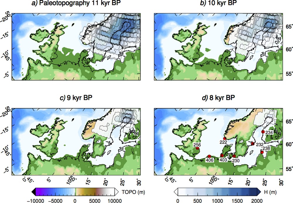
Paleotopography of northern Europe and ice thickness evolution according to model ICE-5G(VM2) in the time window between 11 and 8 kyr BP.
To the east of Doggerland, the evolution of the Baltic Sea during the last deglaciation has been characterised by a complex development of the shorelines, controlled by deglaciation dynamics, isostatic rebound and erosion (Bjorck, 1995). According to the paleotopographic reconstruction of Fig. 4, during the time period between 11 and 8 kyr BP, a major reduction of the Würm ice sheet extension occurred, accompanied by a northward migration of ∼ 500 km of its meridional margin. This has caused a differential isostatic adjustment (Bjorck, 1995), which has enhanced the complex evolution of the geographical features in the region (Kostecki, 2014). Fig. 4 shows the late stage of Ancylus Lake, a fresh water lake, just before the transition to the Littorina Sea (Bendixen et al., 2017). According to our GIA model predictions, the Littorina Sea transgression occurred between ∼ 9 and ∼ 8 kyr BP across the Great Belt (see frames c and d), in substantial agreement with the reconstruction of Kostecki (2014).
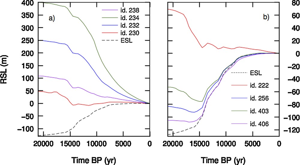
Fig. 5a and b show relative sea-level (RSL) curves for some locations in northern Europe, in the Baltic Sea and in Britain (the locations are marked by red dots in Fig. 4a). The sites are listed in the Tushingham and Peltier (1992, 1993) database, from which RSL data are available. Here, however, we are not concerned with a comparison between model predictions and RSL observations. Rather, we are aimed at assessing the amount of isostatic disequilibrium across the region by a comparison of RSL predictions with the eustatic sea-level (ESL) curve, shown by a dashed line. Due to the strong uplift caused by the melting of the former Würm ice sheet that covered the area at the LGM, RSL curves from the Baltic Sea show a sea-level fall, opposite to the eustatic sea-level increase. The kink at ∼ 14 kyr BP marks the occurrence of MWP-1A, which has caused an accelerated RSL fall in this region. The large isostatic rebound in the Baltic Sea strongly affects the evolution of paleogeography in the area, which confirms the importance of a non-eustatic approach in the definition of aquaterra. In the periphery of the former Doggerland (id. 256, 403 and 406), RSL curves are clearly non-monotonic (Peltier, 1998) and strongly deviate from ESL during the first phase of deglaciation, until MWP-1A. Later on, the RSL curves indicate that isostasy has generally reduced the amount of sea-level rise that we would expect from eustasy, leaving however unchanged the general monotonous trend.
RSL curves at the eight locations shown by red dots in Fig. 4d. ESL (dashed) denotes the eustatic curve.
Fig. 6 shows the late evolution stages of the land bridge that once connected Siberia to Alaska, named Beringia after Hulten (1937). As shown in Fig. 2, this land mass constitutes a sizeable portion of aquaterra. The evolution of Beringia, which had profound implications on human dispersal pattern over North America (see e.g., Clark et al., 2014; Gore, 1997; Hoffecker et al., 2016), has been detailed in a number of studies (see, e.g., Elias et al., 1996; Hopkins et al., 1967; McManus et al., 1983). Of particular interest is the timing of the postglacial flooding of Beringia, which has been long discussed. Based on a well-dated core from the Herald Canyon, very recently Jakobsson et al. (2017) have suggested that the transition from a near-shore environment to an open marine setting occurred ∼ 11 kyr BP, at the time of MWP-1B (see Fig. 3). This fairly agrees with our reconstruction of Fig. 6, showing that the transition occurred between 11 and 10 kyr BP, accompanied by a major disappearance of landmasses from the Arctic Sea. The timing of the flooding event appears to be sensitive to the GIA model employed, however. For example, in Peltier (1998), who adopted the ICE-4G model (Peltier, 1994), the closure of the Beringia land bridge was predicted to have occurred ∼ 9 kyr ago. Computations based on the recent ICE-6G(VM5a) model (Peltier et al., 2015) now support the findings of Jakobsson et al. (2017). To our knowledge, a systematic study of the sensitivity of the time of flooding to the GIA model parameters has not been attempted so far. Using field data, this could potentially provide new constraints on the deglaciation chronology and possibly on mantle rheology.
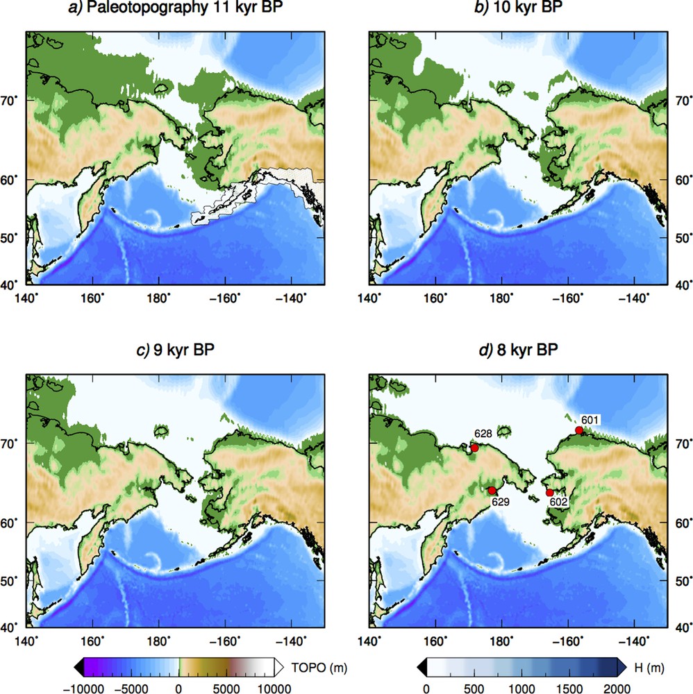
Paleotopography of the Bering Strait between 11 and 8 kyr BP, according to the GIA model computations. The flooding of Beringia occurs between 11 and 10 kyr BP.
In Fig. 7, we show some RSL curves from Alaska (id. 601 and 602 in Fig. 6) and from Eurasia (628 and 629), with coordinates from the Tushingham and Peltier database. Differently from northern Europe (see Fig. 5) in this area the RSL curves are clearly monotonous. Deviations from the ESL curve are large before MWP-1A (∼ 14 kyr BP), but they remain significant also afterwards, especially for sites 601 and 602, located relatively close to the formerly Laurentian ice sheet and thus potentially more affected by isostatic disequilibrium. In particular, site 602 is facing the Bering Strait, adjacent to the place where flooding occurred according to our modelling. This indicates that non-eustatic effects have indeed played a role in the timing of the disappearance of the Beringia bridge (and consequently in the evolution of aquaterra), which supports the argument of Jakobsson et al. (2017) about the importance of isostasy in the region.
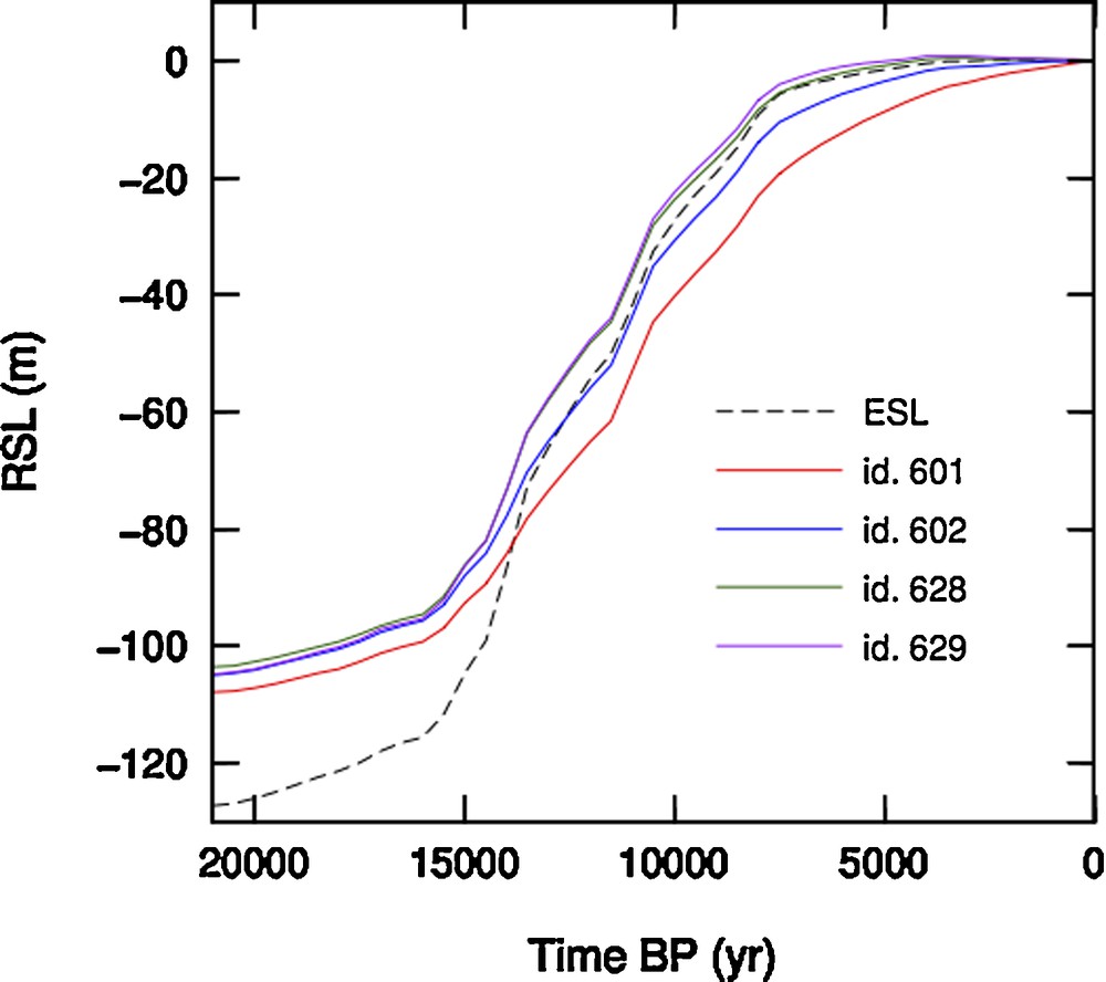
RSL curves from four locations facing the Bering Strait, marked by red dots in Fig. 6. ESL (dashed) is the sea-level curve according to the eustatic theory.
4 Conclusions
Using a GIA model, we have studied the spatial and temporal evolution of aquaterra since the LGM. The SLE has been solved assuming the global deglaciation model ICE-5G(VM2) of Peltier (2004) and taking into consideration all the physical processes that account for non-eustatic sea-level changes. Our conclusions can be summarised as follows:
- i) Dynamic effects play an important role in the evolution of aquaterra, particularly above 45°N. When they are taken into account, the extension of exposed aquaterra is decreased by ∼ 25% with respect to the eustatic case. This contributes to a better description of the deepest boundaries of aquaterra, i.e. the maximum extent of where humans could have directly influenced the landscape
- ii) The history of the size of aquaterra is characterised, between ∼ 14 and ∼ 7 kyr BP by a major reduction, punctuated by abrupt decreases at the time of meltwater pulses MWP-1A, 1B and 1 C. Before MWP-1A and since ∼ 7 kyr BP, changes in the area of aquaterra have been minor
- iii) As expected, dynamic effects associated with GIA play an important role in the evolution of aquaterra in the regions that once were covered by thick ice, like the Baltic Sea region. In the surroundings of Doggerland and across the Bering Strait, they have been less pronounced, but still significant. The timing of the major events like the disappearance of some important aquaterra features like Dogger Island and the Bering Strait bridge appears to the tightly related with MWP-1B (∼ 11 kyr BP). The predicted epoch of these episodes, however, is rather sensitive to the choice of the GIA model.
Acknowledgments
This work is dedicated to Claude Froidevaux, with gratitude for having welcomed GS at the Laboratoire de géologie de l’École normale supérieure (Paris) in 1991 and for a number of very stimulating discussions on several occasions. We are indebted to Luce Fleitout and Jerry Dobson for very valuable comments that have considerably improved the manuscript. We thank Giada Salciccia for her help with the paleogeographic reconstructions. Work funded by research grants of the Department of Pure and Applied Sciences (DiSPeA) of the Urbino University (CUP H32I160000000005). We have used data from the NOAA sea-level database http://www1.ncdc.noaa.gov/pub/data/paleo/paleocean/relativeseaJevel/. Program SELEN can be downloaded from https://geodynamics.org/cig/software/selen/or requested to the authors. The figures have been drawn using the Generic Mapping Tools (GMT) of Wessel and Smith (1998).