

1 Introduction
Sea levels have fluctuated throughout geological time, periodically flooding or draining the world's coastal plains. Sea level is measured with respect to the land surface and any change reflects either a shift in the position of the sea surface or a shift in the position of the land, or both. Causes for this relative sea-level change are several. They include tectonic processes that cause uplift or subsidence of the coastal zone and to an apparent sea-level fall or rise. The observations made by Charles Darwin of fossil seashells and petrified forest trees trapped in marine sediments at elevations of hundreds of meters in the Andes of South America are one example of where the sea-land levels have changed [23]. In this case Darwin actually witnessed the land uplift that occurred during a major earthquake and he was able to conclude that the fossil beds were the result of the cumulative uplift of many large earthquakes over period of time. Sea level also changes if the volume of water in the oceans is augmented or decreased. On very long geological time scales (∼109 years) the ocean volumes probably have increased due to the outgassing of the planet but on the human time scale this is small. Furthermore, sea-level changes when the shapes of the ocean basins are modified during the cycles of sea-floor spreading and plate tectonics on time scales of 107–108 yr. For example, the formation of ocean ridges, or a change in ridge spreading rates, on these time scales result in displacement of water and in global changes in sea level may attain a few hundred meters [18]. More important on a time scale of the last ∼106 years is the cyclic exchange of mass between the ice sheets and the oceans [33]. The ice sheets at the last peak in glaciation contained about 55×106 km3 more ice than today and sea level on average was raised by about 130 m during the deglaciation phase. But the observed sea-level response exhibits a more complex behaviour because of the interactions between ice and land.
The large ice sheets that formed over northern Europe and North America weighed down on the Earth's crust causing it to subside by hundreds of meters. Then when the ice sheet melted the reverse occurred, the deglaciated crust rebounded and sea level locally fell. This is illustrated by the many stranded harbours of the Gulf of Bothnia and gave rise to the concept that the Baltic was drained by subterranean tunnels either into the North and Arctic Seas or into the mantle [3,24]. The loads generated by the changing ice load on the continents and by the concomitant change in water load in the oceans stress the entire planet and change its shape, including that of the ocean basins, in phase with the growth and decay of the ice sheets, and the resultant relative sea-level change is a function not only of the change in ice volume but also of the planet's rheology. Another way to change sea level is to redistribute water mass within the ocean basin. For example, winds from a constant direction may result locally in periods of anomalous sea level. This is seen in the Baltic when arctic winds blow persistently from the northeast and the Baltic water level is systematically lowered by as much as a meter [15]. These meteorologically-driven changes occur on time scales of years and shorter. Differential warming of the oceans, by altering the ocean density structure through thermal expansion also contributes to sea-level change and this is one of the major contributors to change in recent decades [10].
As a result, sea-level change occurs with a complex spatial and temporal spectrum that contains within it a wealth of information on processes operating on the planet: on tectonic processes that cause the uplift or subsidence of the shorelines, on the magnitudes and timing of past glacial cycles, on the deformational physics of the solid part of the planet, and on the meteorological and oceanographic forcing of the sea surface.
2 Observational evidence
Fig. 1 illustrates the time dependence of sea level on three different time scales. The first result is a measure of the global fluctuations in ocean volume for the past 600 million years. On this scale the major oscillations are associated with changes in the ocean configuration due to continental break-up and ocean-ridge formation. The second result in Fig. 1 is for the past 140 000 years and spans the last glacial cycle. The observed fluctuations reflect the cycles of ice growth and decay from the end of the penultimate glacial maximum (∼140 000 years ago), through the last interglacial (∼130 000–118 000 years ago), through the build up to the next peak of glaciation (∼30 000–20 000 years ago) and into the present interglacial period. The third result illustrates instrumental records from two of the longest and most complete tide-gauge records available [10]. These reflect the high-frequency fluctuations of atmospheric and oceanographic origin and possibly the onset of the greenhouse-induced rise starting late in the 19th century.
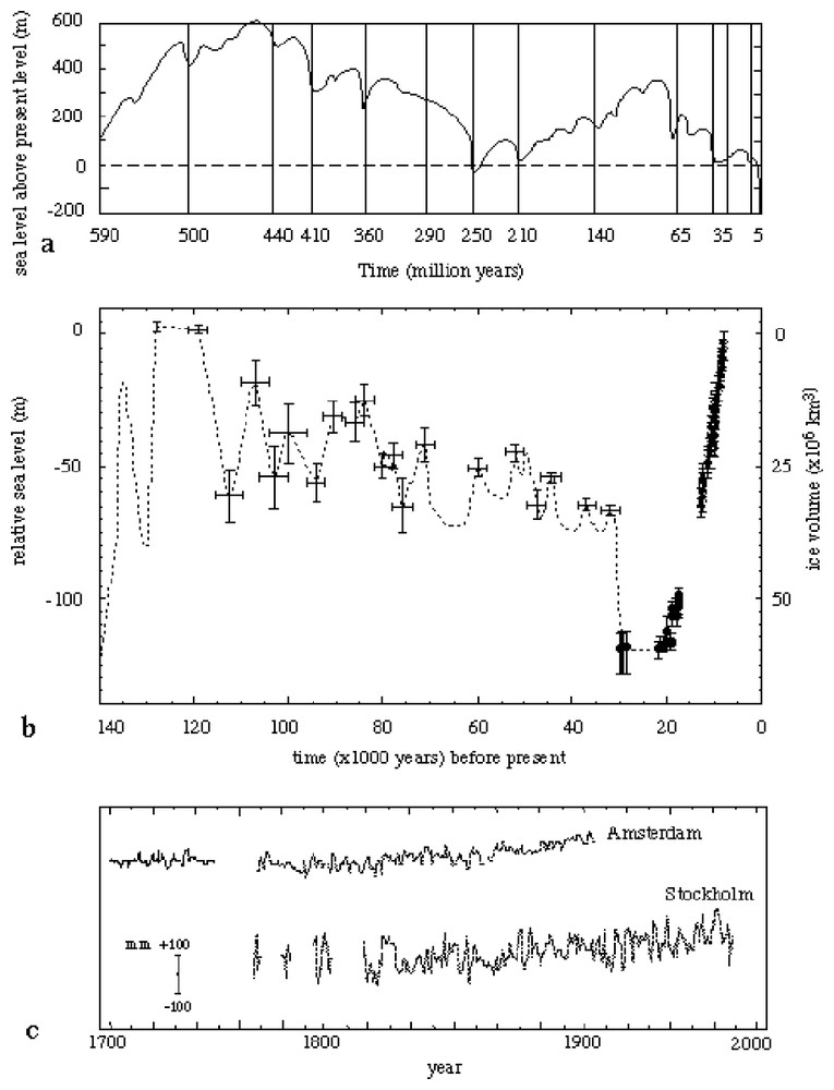
Observations of sea-level change on three different time scales (modified from [33]). (a) Global change for the past 600 Myr as inferred from seismic sequence stratigraphy [18]. The major oscillations are global in origin and probably associated with changes in the ocean basin shape due to continental break-up and ocean-ridge formation. (b) Sea level change during the last glacial cycle as recorded at the Huon Peninsula, Papua New Guinea [33,40]. The part of the records for the Last Glacial Maximum is from the Bonaparte Gulf, northwestern Australia, corrected for the difference in isostatic response (see below) between the two locations. The fluctuations observed here are primarily the results of the changes in high-latitude continent-based ice volume. The change in ice volume, with respect to present-day volume, is indicated by the right-hand scale. (c) Sea level change on century to annual time scales as recorded at two tide gauges [10]. The Stockholm record has had a secular fall in sea level of 4 mm year−1 removed. This is attributed to the glacial isostatic rebound of Scandinavia (see below). The high-frequency changes are of climate and meteorological origin. The apparent small secular change starting in the latter part of the 19th century may be the impact of industrialization on climate.
Observations du changement du niveau de la mer à trois échelles de temps différentes (modifié à partir de [33]). (a) Changement global pour les 600 derniers millions d'années, à partir de la stratigraphie séquentielle sismique [18]. Les oscillations majeures sont d'origine globale et probablement associées aux changements de forme du bassin océanique, dus à la fragmentation des continents et à la formation de la dorsale océanique. (b) Changement du niveau de la mer pendant le dernier cycle glaciaire, tel qu'il est enregistré à la Péninsule Huon, Papouasie-Nouvelle Guinée [33,40]. La partie relative au dernier maximum glaciaire concerne le golfe Bonaparte (Nord-Ouest de l'Australie) ; elle est corrigée de la différence dans la réponse isostatique (voir plus bas) entre les deux endroits. Les fluctuations observées sont majoritairement le résultat des changements du volume actuel sur les continents de haute latitude. Le changement de volume de glace par rapport au volume actuel est indiqué par l'échelle de droite. (c) Changement du niveau de la mer à l'échelle du siècle jusqu'à l'année, tel qu'il a été enregistré par deux marégraphes [10]. L'enregistrement de Stockholm a eu une chute séculaire du niveau de la mer de 4 mm an−1 écartée. Ceci est attribué au rebond isostatique glaciaire de la Scandinavie (voir plus bas). Les changements de haute fréquence sont d'origine climatique et météorologique. Le petit changement séculaire apparent qui débute dans la dernière partie du XIXe siècle pourrait représenter l'impact de l'industrialisation sur le climat.
Observations of sea-level change are most complete for the period after the last deglaciation and Fig. 2 illustrates some representative results. An immediate observation is that almost no two observations are the same, despite all sites represented being considered to be tectonically stable. Various sea-level indicators have been used but all are characterised by measurements of the age and position of fauna–flora fossil or sediment deposits that formed close to or within the tidal range at their time of growth. Data from the Bonaparte Gulf of northwestern Australia indicates that here the levels were at their lowest from about 30 000 to 20 000 years ago, locally some 120 m lower than today, and that the periods immediately before and after experienced rapid change [56]. The evidence for the rise is supported by the data from Barbados and the Sunda Shelf, with both data sets indicating that this was not at a constant rate in the interval from about 20 000 to 7000 years ago [2,19]. In contrast, in both the Gulf of Bothnia and Hudson Bay, sea level has been falling quasi-exponentially by more than 200 m since the areas became ice free [44,55] while at the northwest Norway site of Andøya the change is one of alternating falling and rising levels for the past 20 000 years [54]. The 8000-year result from the Vestfold Hills of Antarctica shows a similar result to the latter part of the Andøya record with a plateau at about 7000 years ago followed by a falling sea level [58]. Along the shores of the North Sea, southern England and the French Atlantic coast – typified by the Bristol Channel observations [21] – sea levels throughout the past 20 000 years were below their present level, with the rate of rise decreasing from the past to present. Along the low-latitude continental margins of Africa and Australia, however, sea levels initially rose until about 7000–6000 years ago and then slowly fell to their present position, the latter part of the record being typified by the result from North Queensland.

Observed sea-level change since the time of the Last Glacial Maximum at different locations around the world [2,19,21,44,54–56,58]. All the sites are tectonically stable except for Barbados where a correction for tectonic uplift has been applied. Note the different time and amplitude scales (after [33]).
Changements du niveau de la mer observés depuis le dernier maximum glaciaire à différents endroits du monde [2,19,21,44,54–56,58]. Tous les sites sont tectoniquement stables, excepté dans le cas des Barbades, où une correction pour la surrection tectonique a été appliquée. A noter les différentes échelles de temps et d'amplitude (d'après [33]).
There is rhyme and reason behind this seemingly curious behaviour of sea level, namely the glacial cycles. Three factors contribute.
- (i) As ice sheets grow and decay the ocean volumes change and sea levels rise or fall.
- (ii) But the ice–water loading of the planet is modified and the surface, including the floor of the ocean basins, deforms and changes the position of the sea surface relative to the land. This deformation is most significant beneath the ice sheets but the loading of the ocean basins by the meltwater (or by the removal of water to the ice sheets) is also a contributing factor.
- (iii) Furthermore, as the ice–water mass is redistributed and the earth deforms, the gravitational potential of the earth–ocean–ice system is modified and sea level, being on average an equipotential surface, is modified: levels near a growing ice margin, for example, rising relative to levels far from the ice.
Thus the relative sea-level response to changes in the ice sheets is the sum of these three contributions whose importance varies with position relative to the ice and water loads. It is this that determines the observed spatial variability illustrated in Fig. 2.
3 Sea level during Glacial cycles
When subject to forces or loads, the Earth deforms. One example is the deformation of the solid part of the planet under the small-amplitude periodic gravitational attraction of the Moon and Sun on the planet. At high-frequency forcing, the response is predominantly elastic but it becomes increasingly viscous as the duration of the load or force increases. At the typical duration of the glacial cycles the response occurs primarily as viscous flow in the mantle and results in both a deformation of the surface of the solid earth and in a redistribution of mass within and on the planet. Sea-level change during a glacial cycle, therefore, is a result of the fluctuations in the volumes of water periodically locked up in or released from the continental ice sheets, of the radial displacement of the surface of the Earth including the deformation of the ocean basins, and of the changing gravity field. Schematically this relative sea-level change can be written as [33,36]:
| (1) |
The first term is the ice-volume-equivalent sea-level change and relates directly to the changes in ice volume ΔVi as [36,41]
| (2) |
In areas of former glaciation, it is the glacio-isostatic term that is most important. At the end of a long glaciation the crust beneath the ice has been depressed by an amount approaching the local isostatic limit of −(ρi/ρm)hi where ρm is the density of the mantle and hi is the ice thickness. Mantle material flows away from the stressed region and within the spherical earth a broad shallow zone of crustal uplift forms. When this ice melts, the formerly loaded crust rebounds and |Δζi|>|Δζe|>|Δζw| and the total sea-level change is dominated by Δζi and Δζe with the two terms being of opposite sign (Fig. 3). This corresponds to the observational signal observed within the Gulf of Bothnia (Ångermanland) or within Hudson Bay (Richmond Gulf). Near the margins of the former ice load the amplitudes of these two terms are more comparable and the sign of their sum varies with time. The resulting signal is characteristic of the Norwegian margin or of Scotland. Outside of the ice margin, on the broad zone of crustal uplift, |Δζe|>|Δζi| and the two terms are of the same sign. Sea-level change here is therefore one of a constantly rising level up to the present and this is characteristic of the change observed in southern England.
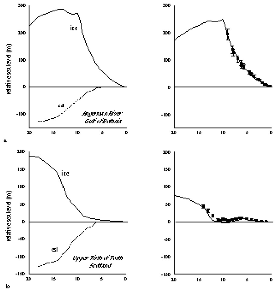
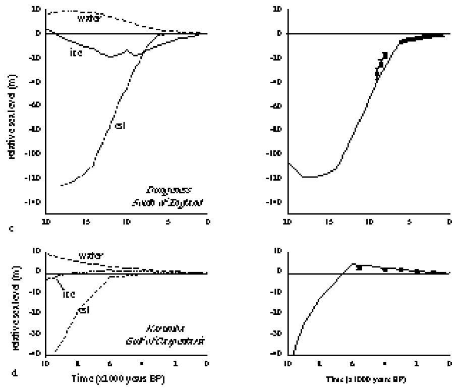
Schematic representation of relative sea-level change as the sum of the principal components Δζe,Δζi,Δζw (labelled as esl, ice and water respectively) (from [30]). The principal components are shown in the left panels and the combined total result, together with the observed values for the site are shown in the right panels. (a) |Δζi|>|Δζe|⪢|Δζw| and the resulting sea level signal is representative of the Bothnia and Hudson Bay sites. This example corresponds to the Ångerman River, Sweden. (b) |Δζi|≈|Δζe|>|Δζw| and the sea-level signal is representative of the Andøya site. This example corresponds to the upper Firth of Forth, Scotland. (c) |Δζe|>|Δζi|>|Δζw| with both Δζe and Δζi of the same sign. The resulting sea level signal is representative of the Bristol Channel data. This example corresponds to Dungeness, England. (d) |Δζw|>|Δζi|>Δζe for the Late Holocene time while for Early Holocene |Δζe|>|Δζw|>|Δζi|. This results in the Late Holocene sea-level highstands that are characteristic of Orpheus Island, Australia, but this result is for Karumba in the Gulf of Carpentaria, Australia, where the amplitude of the highstand is enhanced by the geometry of the coastline such that the site lies at some distance from the open-ocean water load.
Représentation schématique du changement relatif du niveau de la mer comme la somme des principaux composants Δζe,Δζi,Δζw (marqués en tant que esl, glace, eau, respectivement) (d'après [30]). Les principaux composants sont présentés sur les diagrammes de gauche et le résultat total, combiné avec les valeurs observées pour le site, est présenté sur les diagrammes de droite. (a) |Δζi|>|Δζe|⪢|Δζw| et le signal du niveau de la mer résultant est représentatif des sites de Bothnia et de la baie d'Hudson. Cet exemple correspond à la rivière Ångerman, en Suède. (b) |Δζi|≈∣Δζe|>|Δζw| et le signal du niveau de la mer est représentatif du site d'Andøya. Cet exemple correspond à la partie supérieure de l'estuaire de Forth, en Écosse. (c) |Δζe|>|Δζi|>|Δζw| avec Δζe et Δζi de même signe. Le signal du niveau de la mer résultant est représentatif des données obtenues sur le canal de Bristol. Cet exemple correspond à Dungeness en Angleterre. (d) |Δζw|>|Δζi|>Δζe pour l'Holocène récent, tandis que pour l'Holocène inférieur, |Δζe|>|Δζw|>|Δζi|. Ceci résulte, à l'Holocène tardif, en hauts niveaux qui sont caractéristiques de l'ı̂le Orpheus, en Australie, mais ce résultat concerne Karumba, dans le golfe de Carpentaria, Australie, où l'amplitude du haut niveau est accentuée par la géométrie du littoral, de telle sorte que le site est localisé à une certaine distance de la charge d'eau de l'océan ouvert.
The magnitude of the water load term is of the order −(ρw/ρm)Δζrsl and can be expected to contribute about 10–15 m to sea levels for the time of maximum glaciation. Though small, for localities far from the former ice margins |Δζe|>|Δζw|>|Δζi| and the water load term becomes the dominant perturbation in the sea-level signal. This produces the characteristic highstands in Late Holocene time illustrated in Fig. 2 for Orpheus Island, Australia, or in Fig. 3 for Karumba in the nearby Gulf of Carpentaria. During the phase of deglaciation the dominant signal here is the eustatic sea-level rise, superimposed upon which is the viscous subsidence of the sea floor caused by the increased water load, a subsidence that drags the coastline down with it. When melting has ceased this latter signal dominates and results in the observed fall in level up to the present.
4 Earth rheology and ice-sheet dimensions
To solve the sea-level equation (1) the requirements are (i) a set of model parameters defining the earth's rheological response to loading, (ii) a model for the advance and retreat of the ice sheets and (iii) a model for the time dependence of the ocean basin shape. The last of these is provided as a first approximation by the present description of the ocean-land boundaries and water depths and this is then refined by the successive iterations of (1). The elastic parameters defining the earth response are known from seismic studies [14], but the viscosity layering is usually assumed to be only partly known. The final retreat of the ice over the northern continents is reasonably well understood but its retreat over the continental shelves is less well recorded. Also its thickness and its earlier history are not well known. Thus the ice load cannot be assumed known and observations of sea-level change are important in the inversion of (1) not only for parameters that describe the rheology but also for those that define the ice sheets. Such inversions can proceed in an iterative manner to ensure that the ice–earth parameters are effectively separated.
Consider observations from distant sites such as the Bonaparte Gulf and the Sunda Shelf (Fig. 2). These, in a first approximation, establish the total ice volumes during the glacial maximum and the Late Glacial phase. Small isostatic corrections need to be made (the Δζw and Δζi terms) and a preliminary earth model is used for this. The resulting total ice volume needs to be distributed between the major ice sheets and this is done using preliminary ice sheet models that are consistent with the observed ice-retreat history and with the condition that the total ice volume is consistent with the observed global sea-level change. At the sites far from the ice margins the principal sea-level signal for the post-glacial stage is due to the water loading term and this is not strongly dependent on the source of the meltwater, only on the total amount. Observations from localities such as Australia are then used to estimate the mantle rheology [27,31], which, once determined, is used to refine the isostatic corrections. The sea-level data from the formerly glaciated regions is then used to constrain the ice model on the assumption that the rheology from the distant sites provides a useful first approximation of the local rebound and with the constraint that their total ice volume is again consistent with the observed global changes in sea level. These inversions can be complemented with other data sets of the Earth's response to the glacial unloading, including changes in the Earth's rotation and perturbations in the orbits of close-earth satellites [26,36,48], and geodetic measurements of modern sea-level change and crustal deformation [35,45]. By starting from the better-known ice sheets, such as that over the British Isles and Scandinavia, consistent solutions for both ice-sheet and earth–rheology parameters can be established [34,37]. The latter then provide the basis for analysing the ice histories for less well-documented regions such as Arctic Europe and Russia or Antarctica [28].
The principal earth–rheology results from these inversions include evidence for a marked depth dependence of the mantle viscosity, with the average lower mantle viscosity being about 20–50 times higher than the average upper mantle viscosity. Within the upper mantle, some depth dependence also occurs with the seismic transition zone between ∼400 and 670 km depth having a higher viscosity than the upper zone. The effective elastic thickness of the overlying lithosphere appears to be in the order of 65–80 km for most of the continental regions [31,34,37]. There is growing evidence that these average parameters are laterally variable [33,40]. The average upper mantle viscosity, for example, may range from about 1020 Pa s or less beneath the South Pacific lithosphere to about (5–7)×1020 Pa s beneath North America but mostly either the observational evidence or the a priori information on the ice loads is inadequate to attempt formal solutions for lateral variability. Thus the above results are based on regional analyses using radially stratified models. The second major assumption, linearity of the response function, also remains to be verified but currently all data for rebound are consistent with this hypothesis.
Even without formal inversions, the observational data provides a quick indicator of the nature of the ice sheet limits. The Andøya result (Fig. 2) of well-elevated shorelines at about 19 000 years ago, for example, indicates that at some earlier time the ice margin must have stood offshore so as to produce sufficient rebound to leave raised shorelines today.
Thus the ∼10 000 year old elevated shorelines observed at many localities in Svalbard (including Hopen and Kong Karls Land) [16] indicate that before that time a substantial ice sheet was centred over the Barents Sea and that it extended out to the western and northern shelf edge. The absence of such shorelines along the southern shores of the Kara Sea indicates that any such ice sheet over Arctic Russia must have been much older than the time of the last peak in glaciation [28]. The well-elevated shorelines of Baffin Island [1] dictate that the ice margin here at the time of the Last Glacial Maximum (LGM) stood at the edge of the shelf in the Davis Strait [39]. Likewise, the rebound of segments of the Antarctic coast where old rock surfaces are exposed indicates that here also the ice stood further offshore and was thicker than it is today [59].
If the ice margin locations are known, then the inversions of sea-level data do appear to yield reliable parameters for earth rheology and ice thickness provided that the observational data is well distributed around the former ice margins and provided that the data extends back into early Lateglacial time. This is the case for both Scandinavia and the British Isles but less so for North America and not at all so for Antarctica. For Scandinavia, the inversion results indicate that the Lateglacial ice thickness was relatively thin (∼2000 m) when compared with ∼3500 m for the classic ice sheet models [13], particularly in the southeast and south [37]. A few records for earlier epochs, e.g., Andøya, indicate that during the early part of the LGM the ice thickness was greater than this and that a rapid reduction occurred in early Lateglacial time with the eastern part of the ice sheet becoming unstable at about 19 000–18 000 years ago [38]. Inversions of the data in which the coupling of the ice to the underlying bedrock is assumed to be time and position dependent are currently under investigation and the preliminary results are consistent with a model in which cold basal conditions occur initially but that in the eastern half and in the south they become warm based in Lateglacial time, not inconsistent with field data [25].
5 Rapid sea-level change before the Last Glacial Maximum
Fig. 1(b) illustrates the sea-level oscillations during the glacial cycle as recorded in the raised coral reefs of the Huon Peninsula, Papua New Guinea. This is a region of tectonic uplift at rates approaching 4 mm yr−1. Coral growth proliferates when the rate of sea-level rise equals or exceeds the rate of land uplift but when the rise cannot keep up only thin veneers of coral develop. Thus many of the relative highstands in sea level are recorded by well-developed reef structures, the number of the reefs increasing with rate of uplift as more oscillations in sea level are recorded. Huon terraces of last interglacial age now occur up to 400 m above sea level whereas in tectonically stable areas they lie only a few meters above present sea level. This difference yields the average uplift rate and hence the positions of sea level at the times of reef development. The timing of the reef growth is determined by high-precision uranium-series dating [5,7]. The intervening lowstands have been inferred from delta sequences formed by rivers flowing from the hinterland although these estimates are of lower precision than the highstands [4]. These results represent the local sea-level oscillations but because the site lies far from any former ice margins they are representative of sea-level change along low-mid latitude continental margins. They have been supplemented here by the glacial maximum sea levels from the Bonaparte Gulf in which the latter have been corrected for the small difference in isostatic response at the two sites. Holocene information from the Huon location has also been included [6]. Following the above sketched-out process for estimating the isostatic corrections, the ice-volume-equivalent sea level Δζe is estimated, or equivalently the change in grounded ice volume from (2) (Fig. 1(b)) where the ice volume at any time t includes land based ice and ice grounded on the continental shelves but below sea level. It does not include floating ice [41].
The last interglacial (Marine Isotope Stage 5e, MIS-5e) is defined by a period of global reef growth at levels near present sea level, although, analogous to the Holocene, the onset of interglacial climate conditions will have occurred a few thousand years before reef growth first occurs at the present level. Detailed analyses of the reefs of both Huon and Barbados indicate that the oscillations in sea level during substages 5d–5a are actually more complex than shown here [50] but the essential features of periods of reef growth during the interstadials 5c and 5d, separated by relative low stands, are well recorded at all sites. They point to a rapid transition from interglacial to cold conditions with global ice volumes about 30% of the additional ice at the time of the LGM and with equally rapid decreases and regrowth of the ice. The transition to the stadial 5d, for example, suggests that ice volumes of as much as 20×106 km3 can form in less than 10 000 years. Where this ice formed remains uncertain but the most probable location is over Arctic Russia rather than Scandinavia, and over Arctic Canada rather than over the more southern latitudes of the LGM ice [11,53].
The cold period of MIS-3 is characterised by a time of rapid oscillations in sea level with the implication that the ice-volume responses to fluctuations in climate were rapid and substantial. Within dating precision, the timing of the highstands within this interval, at 32, 36, 44, 49–52, and 60 thousand years ago, coincide with variations in ice-rafted debris deposition noted in both the North and South Atlantic Oceans (the Heinrich events [20]) and this suggests a close relationship between periods of reef growth at Huon and the climate signals in the marine sediments of the Atlantic: reef growth occurs in response to rising sea level caused by ice-sheet collapse during or at the end of cold periods [8,39,57]. If this correlation is accepted then the best chronology for the Heinrich events is the U-series ages for the Huon terraces.
6 Palaeoreconstructions of coastal zones
Once earth and ice models have been established from sea level and other rebound data, it is possible to predict the evolution of shorelines and bathymetry through time, particularly for period since the time of the LGM. If the elevation (or depth) of a point at the present time is h(t0) and the sea-level change since a time t is Δζrsl then the elevation (or depth) at t is
The locus of h(t)=0 determines the location of the shoreline at time t. The δh is a correction for any erosion or sedimentation that may have occurred in the interval t−t0.
Examples of past shoreline reconstructions are illustrated in Fig. 4. All epochs are in calendar years. The Persian Gulf result is for 14 000 yr ago when the Gulf was much reduced in size with the Tigris–Euphrates River system connecting marshlands and shallow lakes as it meandered to the open sea at Hormuz [29]. The next 7000 years would have been a time of rapid flooding of the valley. Did this now-flooded valley form the route travelled by the ancestors of the Sumerians [52]. At 7000–6000 years ago the local sea levels were a little higher than present, analogous to the Australian coastal examples, and Hammar Lake formed a shallow extension of the Gulf. The Sumerian sites of Obeid, Ur and Erridu would therefore have been close to the coast, as recorded in the cuneiforms [22]. It becomes tempting to associate the Sumerian flood and the legendary struggles with the sea [51] with the peak of the Holocene transgression and the preceding period of constant encroachment of the sea.
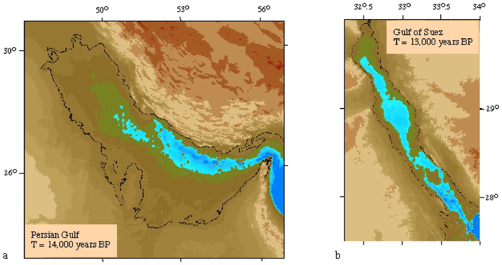

Palaeogeographic reconstructions for four regions. (a) The Persian Gulf at ∼14 000 years ago [29]. Before this time the Euphrates–Tigris River system flowed via a series of lakes and low depressions to reach the sea at the Strait of Hormuz. (b) The Upper part of the Red Sea and the Gulf of Suez at ∼13 000 years ago. Throughout the glacial cycle the Red Sea remained open to the Indian Ocean at its southern end, but the Gulf of Suez was periodically dry. The topographic barrier at the southern end of the Gulf, if preserved during the glacial cycle, could result in catastrophic flooding when sea level exceeded the barrier just before 13 000 years BP. (c) The Cycladean islands in the Aegean Sea at ∼16 000 years ago when the Cycladean plateau was still near its maximum extent of LGM time. This large land mass included the now islands of Ándros, Tı́nos, Mikonos, Páros, Náxos and Íos, which rose as mountains above a flat-lying plain. It was separated from the mainland at Evvoia and from the western Cycladean islands, including Mı́los, by narrow channels that could be crossed without loosing sight of land on either side [30]. By about 14 000 years ago, the island began to founder and the present-day islands were mostly separate entities by about 12 000 years ago. (i) Mı́los, (ii) the Palaeolithic site of Franchthi where obsidian from Mı́los has been found. (d) The palaeogeographic reconstruction of the Sicilian Channel between North Africa and southern Italy at the time of the Last Glacial maximum [42].
Reconstitutions paléogéographiques pour quatre régions. (a) Golfe Persique il y a 140 000 ans [29]. Avant cette époque, le système fluvial Tigre–Euphrate coulait au travers d'une série de lacs et de dépressions basses, pour atteindre la mer au détroit d'Hormouz. (b) Partie haute de la mer Rouge et du golfe de Suez, il y a 130 000 ans. Au cours du cycle glaciaire, la mer Rouge est restée ouverte sur l'océan Indien à son extrémité sud, mais le golfe de Suez était périodiquement sec. La barrière topographique à la partie sud du golfe, si elle a été préservée pendant le cycle glaciaire, a pu donner lieu à une inondation catastrophique quand le niveau de la mer dépassait la barrière, juste avant 13 000 ans BP. (c) Îles Cyclades dans la mer Égée il y a 16 000 ans, lorsque le plateau cycladique était encore porche de son maximum d'extension au temps LGM. Cette grande masse continentale comportait les ı̂les actuelles d'Ándros, de Tı́nos, de Mikonos, de Páros, de Náxos et d'Íos, qui s'élevaient telles des montagnes au-dessus d'une plaine plate ; elle était séparée de la terre ferme à Evvoia et des ı̂les occidentales des Cyclades, incluant Mı́los, par des chenaux étroits qui pouvaient être traversés sans perdre de vue la terre de chaque côté [30]. Il y a environ 14 000 ans, l'ı̂le a commencé à s'enfoncer et les ı̂les actuelles sont, pour la plupart, des entités séparées, à environ 12 000 ans. (i) Milos, (ii) le site paléolitique de Franchthi, où l'obsidienne de Milos a été trouvée. (d) Reconstitution paléogéographique du canal de Sicile entre l'Afrique du Nord et le Sud de l'Italie au dernier maximum glaciaire [42].
The second example is from the Red Sea. No land bridge developed at the southern end at any time during glacial lowstands, although this entrance was considerably constricted at these times. The Gulf of Suez, however, was above sea level, with a sill at its southern margin which would have been breached just before 13 000 years BP, resulting in a rapid flooding of the gulf floor. This, of course, is much too early for the traditional timing of the Moses legend but could this story have its origins in a distant memory of a much earlier flooding event.
The third example is from the Aegean where, during times of lowstand, the Cycladean islands formed a large plateau above sea level separated from the mainland by only a narrow channel, which could be crossed without loosing sight of land on both sides. As sea level rose, the plateau gradually broke up to reach its present collection of islands at about 12 000 years ago [30]. Can this have been Plato's Atlantis? The timing of the break-up and description of the island before break-up is not at variance with Plato's account [43] but its veracity requires long preservation of mythologies. Possibly more serious is the occurrence on the mainland of obsidian from Mı́los before 12 000 years ago [9]. With these reconstructions it becomes clear that it would not have required particularly sophisticated sailing skills, as sometimes suggested, to travel between the source and final resting place of the volcanic glasses, it being possible to cross the two occurring water channels without loosing sight of either shore at any time during the crossings.
The fourth example is for the area between North Africa and southern Italy. Here the waters are sufficiently deep for an open channel to remain between Africa and western Sicily at times of lowstand with the island of Pantelleria forming a convenient beacon, closer to Sicily than Africa [42]. The minimum crossing between Tunisia and Pantelleria was about 70 km and, with an elevation of more than 600 m above then sea level, the island would have been just visible from the African shore. These conditions persisted for the long interval of the last cold period from about 33 000 years ago until about 16 000 years ago and also during the cold period preceding the last interglacial. Thus a crossing from Africa to Italy could have been effected during glacial times knowing beforehand that there was land at the other side.
These examples all indicate that significant changes occurred in the geography of both the Mediterranean Basin and the Near East at a time when modern man was exploring the region and laying down the foundations for its legends, the interpretation of which should be done in this palaeogeographic framework rather than that provided by a modern atlas. A predominant effect of the climate change from the ice age to the warmer conditions would have been the rising sea level with the flooding of coastal plains, the loss of access to caves (e.g., Cosquer Cave [12,32] ) and other habitation or work sites (e.g., the submerged sites of Saliagos [46] or the flooded Neolithic settlements offshore Israel [17]) and it is tempting to suggest that the nearly-universal flood myth is the collective but distant memory of a time when coastal campsites had to be regularly displaced to be protected from the persistently advancing sea. It is perhaps notable that the flood legend appears to be absent around the Gulf of Bothnia and northern Baltic shores. Instead, was the whirlpool legend, well illustrated in the annals of 1655 [24], reinforced by a collective memory of falling sea levels?