

1 Introduction
There are two principal types of fractures in geological media and notably in sedimentary basins (reservoirs), joints and shear fractures. The principal difference between them is that shear fractures accommodate shear displacements, whereas along joints only normal to joints displacements are possible. Another difference is in the orientation of fractures compared to the acting (during fracturing) stress directions. Joints are parallel to the most compressive stress σ1 and normal to the least compressive or the most tensile stress σ3. Joints thus make angle ψ = 0° with σ1 and typically are organized in regular parallel (tabular) sets or orthogonal networks. Shear fractures are oblique to both σ1 and σ3 and typically form conjugate networks, oriented to σ1 at angles ψ = ±10°–30°. All fracture types are parallel to the intermediate principal stress σ2.
1.1 Theoretical background of fracture formation
The mechanism of fracture formation remains not completely clear. This is particularly true for joints, which is reflected in different names used for this fracture type: tensile, extension, opening mode or cleavage fractures. Most commonly, they are believed to form (or more exactly, to propagate from a preexisting flaw) according to Mode-I mechanism (Fig. 1) stemming from Linear Elastic Fracture Mechanics (LEFM), (e.g., Lawn, 1993). Accordingly, shear fractures are believed to be Mode-II fractures (Fig. 1). From a theoretical point of view, LEFM is applicable only when the size of the near tip zone (process zone) undergoing inelastic (irreversible) deformation or damage is small compared to other geometric dimensions of the problem (fracture length, size of the deforming object). This assumption can hold only at a relatively low pressure P (or stress level), when deformation and fracture occur in a purely brittle regime. However, this is certainly not the case in the experimental tests at a relatively high P, when damage (revealed by acoustic emissions) involves practically the entire deforming specimen prior to the fracture (e.g., Fortin et al., 2006). In this “ductile” regime, the failure occurs via localization of the initially distributed damage (inelastic deformation) within a narrow band that then can become a fracture. The theoretical framework for addressing the mechanical instability resulting in deformation localization constitutes the bifurcation theory applied to elasto-plasticity models (Chemenda, 2007; Issen and Rudnicki, 2000; Rudnicki and Rice, 1975; Vardoulakis and Sulem, 1995). This theory is completely different from LEFM (which does not explicitly take into account the inelastic deformation), and explains very well the formation of various types of shear deformation bands at the origin of shear fractures. However, the prediction of dilation banding (which can be at the origin of joints, see below) does no go straightforward from this theory when realistic material parameters (notably the dilatancy factor) are adopted.
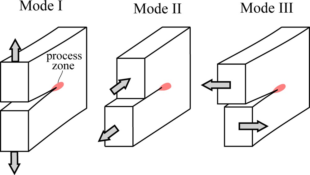
Fracture modes.
1.2 Insights from experimental studies
The transition from very brittle to “ductile” fracturing with increasing pressure has been observed in numerous experimental tests (e.g., Bésuelle et al., 2000; Fortin et al., 2006; Wong et al., 1997) including the conventional (axisymmetric) extension tests on specimens made of Granular Rock Analogue Material (GRAM), which behaves as real rocks, but is much weaker than hard rocks (Nguyen et al., 2011). The dog-bone and cylindrical specimens are first loaded hydrostatically in these tests to a given confining pressure P that is equal to σ1 and σ2, and then unloaded in the axial direction that becomes σ3, P being maintained constant. With increasing P, specimen fracture occurs at progressively smaller |σ3| (which is negative), but the failure plane orientation does not change until σ3 reaches approximately zero (Fig. 2a, b): this plane is parallel to σ1 (ψ ≈ 0°), Fig. 2b, which corresponds to jointing. With further P increase, ψ increases (Fig. 2b), which corresponds to shear fracturing.
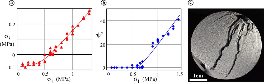
Results from conventional (axisymmetric) extension tests of Granular Rock Analogue Material, GRAM (from Chemenda et al., 2011a). (a) Minimum nominal stress σ3 at fracturing/rupture vs confining pressure or σ1. (b) Angle ψ between the rupture plane and σ1 direction vs σ1 at failure. (c) Surface of the fracture (opened rupture zone) formed at σ1 = σ2 = 0.6 MPa. The initiation point (zone) of the plumose morphology is due to the stress concentration caused by the rigid support of the LVDT gage attached to the specimen (to the jacket) at that location. Masquer
Results from conventional (axisymmetric) extension tests of Granular Rock Analogue Material, GRAM (from Chemenda et al., 2011a). (a) Minimum nominal stress σ3 at fracturing/rupture vs confining pressure or σ1. (b) Angle ψ between the rupture ... Lire la suite
Although the orientation of failure planes in the stress space in GRAM experiments is the same (ψ ≈ 0°) within the P range of joints formation, the “ductility” of the failure process clearly increases with P, which is expressed in the morphology of the forming fracture surfaces (Chemenda et al., 2011a). At low P, these surfaces are rather smooth, while at high P, they are rough, with the rugosities being organized in nice plumose features (Fig. 2c) so typical for natural joints (e.g., Bahat, 1991; Pollard and Aydin, 1988; Savalli and Engelder, 2005; Woodworth, 1896). The damage/failure process occurs under these pressures within a band of a finite thickness comparable to the plumose relief. This process is therefore rather ductile and is not limited to the opening of a “zero”-thickness plane, which would be the case during Mode-I fracturing. SEM observations of the failure zones forming at high P in GRAM specimens reveal a several grains-thick irregular wavy band of damaged material with increased porosity (Chemenda et al., 2011a). This σ3-normal band can be called a pure dilation band. The conclusion made by Chemenda et al. (2011a, b) is that the jointing mechanism changes from Mode-I cracking to dilatancy/dilation banding with increasing P. With further pressure increase, failure occurs via the formation of shear-dilatant deformation bands.
The dilation banding clearly involves ductile, but also tensile damage/failure mechanisms. This is the reason why the dilatancy banding could not be correctly predicted theoretically from deformation bifurcation analysis within an elasto-plasticity framework as mentioned above. In this paper, we investigate this process numerically by considering both brittle-tensile (BT) and shear-ductile (SD) failure/damage mechanisms.
2 Constitutive formulation
The adequate constitutive formulation is the most important ingredient in theoretical analysis and numerical modeling of inelastic deformation (damage) and failure of geomaterials. Rock mechanics experimental studies with different loading configurations (considerably accelerated recently (e.g., Ingraham et al., 2013; Li et al., 2018; Ma et al., 2017), clearly show the importance of the loading type (controlled by the Lode angle), which affects the mechanical response of rocks. A new constitutive model has been proposed based on these experimental data (Chemenda and Mas, 2016). The model includes a three-invariant yield function
| (1) |
and the related plastic potential (n is the constant scalar that can take values from −0.1 to −1). The bifurcation analysis within the framework of this constitutive model led to the predictions of rock failure regimes that are in good agreement with the experimental data, and that are different from the predictions made based on the classical 2-invariant theories like that of Drucker–Prager (Chemenda and Mas, 2016). Here
| (2) |
It does not include σ2, which is a simplification of reality that can be justified by the experimental fact that the rock properties depend much stronger on σ1 and σ3 than on σ2 (e.g., Ingraham et al., 2013; Ma et al., 2017). The plastic potential function reads
| (3) |
where μc, kc, μβ are the friction, cohesion and dilatancy parameters (not coefficients); A takes value 0 or 1 for the brittle-tensile (BT) and shear ductile (SD) failure/damage mechanisms, respectively. The initial values of μc and kc as well as of the tensile strength σt (
| (4) |
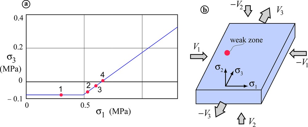
(a) Initial yield surface/envelope or function used in the numerical simulations (simplified plot in Fig. 2a). Points 1 to 4 correspond to the stress states applied in the numerical models. (b) Setup of numerical modeling. The models were pre-stressed to the initial stresses σ1 and σ2 (σ2 = σ1) corresponding to points 1 to 4 in Fig. 3a, and to a sufficiently large σ3 for the model to remain in a purely elastic state. Then σ3 was progressively decreased (by applying velocities V3 to the σ3-normal boundaries), while maintaining the initial values of σ1 and σ2 by applying velocities V1 and V2 as shown in this figure. The model size is 5 × 10 cm (200 × 400 numerical zones) in the σ1 and σ3 directions, and one numerical zone, in σ2 direction. To take into account in the models heterogeneities typical for real rocks, two scale property heterogeneities were introduced in different models (indicated in the captions of the figures showing the corresponding numerical results): (1) Gauss distribution in the numerical zones of the Poisson's ratio with a mean value of 0.25 and standard deviation of 0.02; (2) a weak zone of a larger scale (including several numerical zones) shown in this figure. The strength in this zone is indicated in the captions of the figures presenting the numerical results. Masquer
(a) Initial yield surface/envelope or function used in the numerical simulations (simplified plot in Fig. 2a). Points 1 to 4 correspond to the stress states applied in the numerical models. (b) Setup of numerical modeling. The models were pre-stressed ... Lire la suite
The much higher brittleness of the BT (than that of the SD) mechanism is taken into account in the following softening rules:
| (5) |
where
The elastic properties of the model both before and after reaching the yield condition are described by Hooke's equations with Poisson's ratio ν = 0.25 and Young's modulus E = 6.7 × 10⁸ Pa, characterizing GRAM material (Nguyen et al., 2011).
The formulated constitutive model has been implemented into the finite-difference dynamic time-matching explicit code Flac3D (Itasca, 2012) used for numerical modeling in this work. Numerous simulations were carried out in quasi-static, large-strain mode with different model parameters. Below we report representative results.
3 Setup of numerical modeling
The modeling setup (Fig. 3b) is two-dimensional in the sense that the model thickness in the σ2-direction is only one numerical zone (or 0.25 mm), but the strain rate in this direction is not zero (see below). The model is first pre-stressed to the initial stresses σ1 = σ2 and to a sufficiently large σ3 for the stress state to be above the initial yield envelope in Fig. 3a (this corresponds to the purely elastic mechanical state). Then, σ3 is progressively decreased by applying velocities V3 to the σ3-normal model boundaries, while maintaining the initial values of σ1 and σ2 by applying velocities V1 and V2 as shown in Fig. 3b. In reality, maintained and monitored are averages over each boundary or nominal stresses as it is typically done in the experimental tests. Since V2 is not zero, the models are not plane-strain.
4 Results
We report here the results corresponding to the four points shown on the yield envelope σ3(σ1) in Fig. 3a. The first point (point 1, σ1 = 0.3 MPa; σ3 = −
4.1 Point 1 in Fig. 3a, σ1 = σ2 = 0.3 MPa
4.1.1 Homogeneous model
In this case, the tensile failure occurs exactly at (along) one of the σ3-normal ends of the model due to the end effect. Although very small, this effect exists in the numerical models, and occurs where the extension is applied to the model, i.e. at the σ3-normal boundaries.
4.1.2 “Homogeneously heterogeneous” model with small variations of the Poisson's ratio ν
The Gauss distribution of ν is applied in this model with a mean value of 0.25 and a standard deviation of 0.02. This leads to a non-uniform stress distribution during the loading, which eliminates the boundary (end) affects because the stress perturbations within the model are larger than those (very small) caused by these effects.
Fig. 4 shows the evolution of fracturing, which occurs exclusively according to the BT mechanism as expected (Fig. 4e); the SD mechanism was not activated at all. The formed tensile fractures constitute a generally normal to σ3 but rather irregular set. This is because the model is almost homogeneous and therefore fracturing is initiated simultaneously in different points resulting in stress drops and perturbations of the stress field. Therefore, the initiated fractures propagate in the heterogeneous field, which explains their irregular geometry. To avoid such multiple stress perturbations, in the following model a small weak zone is introduced.
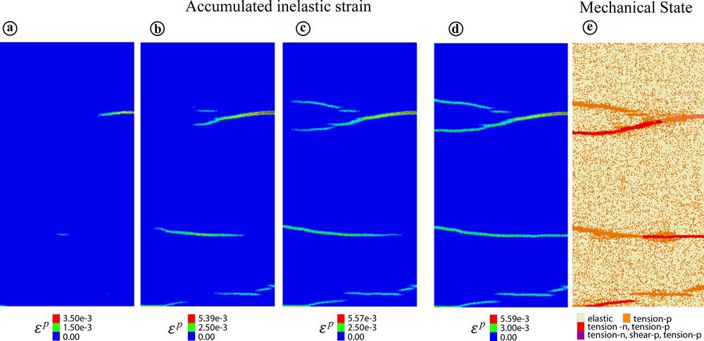
(a–d) Evolution of the inelastic strain, ɛp, pattern during vertical unloading (σ3 reduction) of the model at constant σ2 = σ1 = 0.3 MPa, corresponding to point 1 in Fig. 3a. Poisson's ratio ν varies in the numerical zones according to Gauss distribution. (e) Mechanical state (elastic and elastic-plastic), damage/failure or inelastic deformation mechanism (tensile or shear) and its history for the deformation stage in (d). Different colors in this image correspond to different damage/failure mechanisms and their succession. For example, “tensile-n (n means now), shear-p, tensile-p (p means past)” indicates that the corresponding zones undergo tensile damage at the stage shown, but they already underwent shear and tensile damage during the previous deformation stages (in the past). Zones indicated as “elastic” did not undergo inelastic straining at all. Masquer
(a–d) Evolution of the inelastic strain, ɛp, pattern during vertical unloading (σ3 reduction) of the model at constant σ2 = σ1 = 0.3 MPa, corresponding to point 1 in Fig. 3a. Poisson's ratio ν varies in the numerical zones ... Lire la suite
4.1.3 Model with weak zone
This zone is shown in Fig. 3b and can be recognized in Fig. 5a. The strength parameters in this zone are reduced, as indicated in the caption of Fig. 5; the other parameters are the same as in the rest of the model. One can see that the fracturing occurs in this case in a completely different way compared to the previous model in Fig. 4. There is only one fracture that is initiated at the weak zone and propagates strictly normal to σ3. Propagation occurs due to the tensile stress concentration at the fracture tip, where it reaches σt (Fig. 6b). This Mode-I-type propagation occurs exclusively due to the BT failure mechanism, SD mechanism being operated only within the weak zone (Figs. 6c, d).
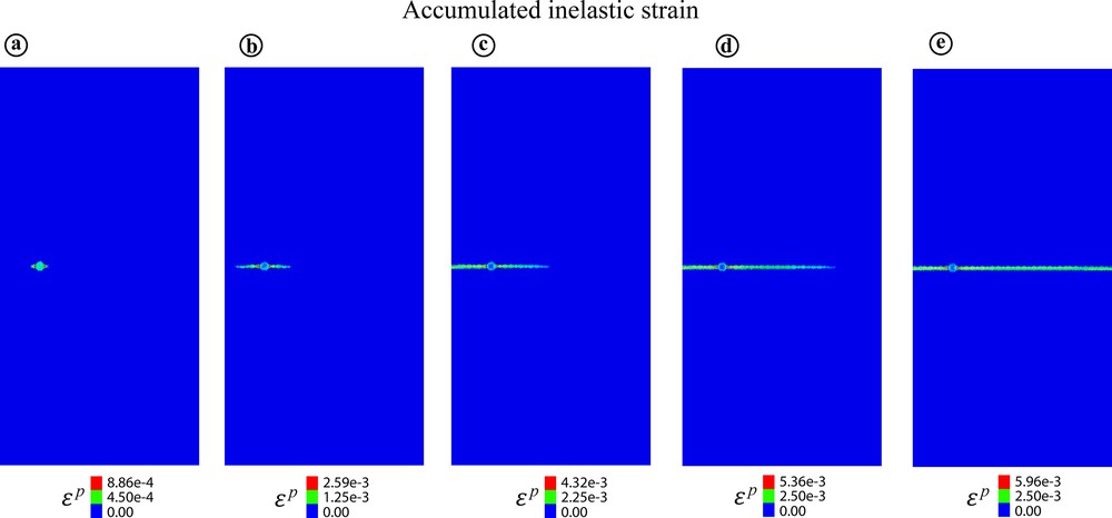
Evolution of the ɛp pattern in the model with Gaussian ν distribution and a weak zone with the reduced initial strength parameters: σt = 0.03 MPa; kc = 0.1 MPa. The initial stresses and boundary conditions are the same as in the previous model.
The inelastic strain ɛp (a), the least stress σ3 (b), and the mechanical state (c) patterns at the same evolutionary stage of the model in Fig. 5; (d) corresponds to the last stage of fracture propagation in Fig. 5e.
4.2 Point 2 in Fig. 3a, σ1 = σ2 = 0.54 MPa
4.2.1 Homogeneous model
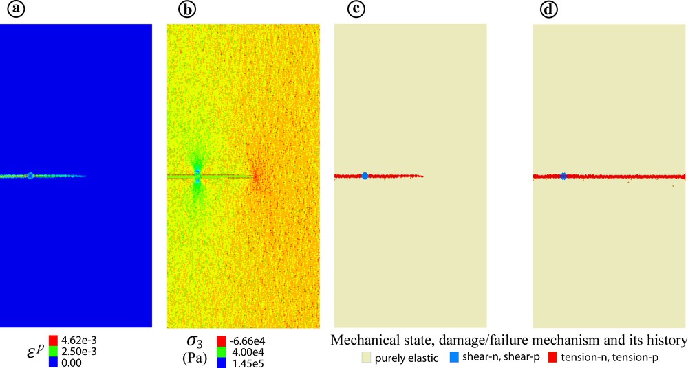
A dense network of conjugate shear bands is first initiated throughout the entire model (Fig. 7a). Then, most initial bands die, while the remaining ones accommodate growing inelastic deformation. This process results in a few principal (well-developed) shear bands (Fig. 7c). One of them then is transferred into three-segment fracture when the BD mechanism comes in play (Fig. 7d, e).
Evolution of the ɛp and mechanical state patterns in a homogeneous model corresponding to point 2 (σ2 = σ1 = 0.54 MPa) in Fig. 3a.
4.2.2 Homogeneously heterogeneous model
Before fracturing, this model undergoes distributed BT, but mostly SD distributed damage (inelastic deformation), Fig. 8a. Then, an oblique fracture is initiated and propagates due to both BT and SD mechanisms (Fig. 8b–d). The oblique fracturing process is followed by an almost σ3-normal one (Fig. 7d).
Evolution of the ɛp and mechanical state patterns in the model with a Gaussian distribution of ν. The initial stresses and boundary conditions are the same as in the previous model (the stress state corresponds to point 2 in Fig. 3a).
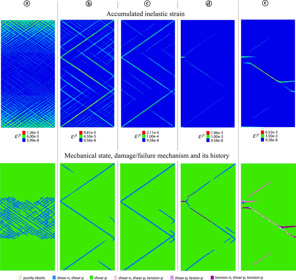
4.2.3 Model with weak zone
The introduction of the weak zone again changes radically the fracture process and geometry (Fig. 9). The fracture propagating from the weak zone does not follow exactly a linear trajectory in this case. Its tip slightly undulates during propagation, resulting in globally σ3-normal macro fracture orientation, whose formation involves both BT and SD mechanisms (Fig. 9). One can recognize both the process (blue dots) and damage (green dots) zones on the maps of damage distribution in Fig. 9 (the second row in this figure).

Evolution of the ɛp and mechanical state patterns in the model with a Gaussian distribution of ν and a weak zone with following strength parameters: σt = 0.03 MPa; kc = 0.3 MPa. The initial stresses and boundary conditions are the same as in the two previous models (the stress state corresponds to point 2 in Fig. 3a).
4.3 Point 3 in Fig. 3a, σ1 = σ2 = 0.6 MPa
4.3.1 Homogeneous model
The deformation pattern in this case is similar to that in Fig. 7, which is explained by the fact that, in both cases, the imposed stress states correspond to the SD domain.
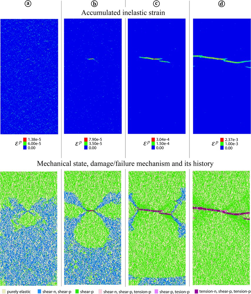
4.3.2 Model with weak zone (Fig. 10)
The result is similar to that in Fig. 9, but the process and damage zones related to the fracture (or more exactly to the deformation band) propagation are much larger. They develop exclusively through an SD mechanism and involve almost the entire model (the last row in Fig. 10). At the band/fracture tip, σ3 is tensile. Its maximum magnitude reaches around 0.06 MPa, which is somewhat less than
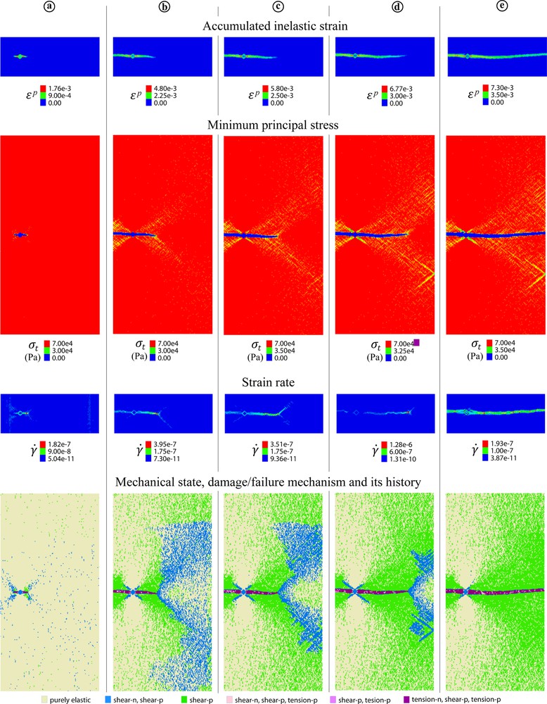
Evolution of ɛp, of the octahedral strain rate
Evolution of ɛp, of the octahedral strain rate
Within the band, both BT and SD mechanisms are active. As in the previous case (Fig. 9), the fracture/band tip undulates during propagation. This time, the reason for this is clear from the octahedral strain rate
4.4 Point 4 in Fig. 3b, σ1 = σ2 = 0.66 MPa
4.4.1 Model with weak zone
The same weak zone as in the previous model leads in this case to the initiation of the σ3-normal extension band (that can hardly be recognized in Fig. 11) and of two conjugate shear bands (Fig. 11a), the latter propagating much faster than the former. Then one shear band dies and the other one cuts the entire model and becomes a shear fracture (Fig. 11e). One can see a large process zone in front of the propagating band (the second row in Figs. 11b–d).
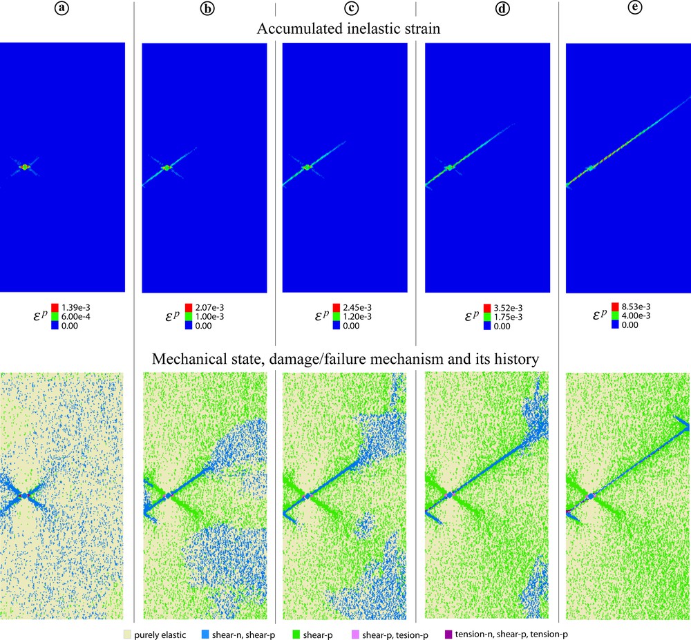
Evolution of the ɛp and mechanical state patterns in the model with Gaussian distribution of ν and a weak zone with σt = 0.03 MPa; kc = 0.3 MPa. The initial stresses correspond to point 4 in Fig. 3a (σ2 = σ1 = 0.66 MPa).
5 Concluding discussion
The reported results show that not only the geometrical attributes of fracture in geomaterials, but the fracture mechanism itself strongly depend on the presence of heterogeneities. Joints, which are believed to be Mode-I fractures, are supposed to form exclusively when the tensile stress σ3 reaches the tensile strength σt (or more exactly, when the stress intensity factor reaches a critical value). This concept works fairly well for purely tensile fractures forming according to the brittle-tensile (BT) deformation/fracture mechanism. This mechanism is possible at a relatively low far-field stress level (or pressure P), when the inelastic process zone near the fracture tip is very small as in Figs. 5 and 6. However, when P is high enough (compared to
The numerical models thus predict a complication of the fracture process and roughening of the joint surfaces (walls) with increasing P. This is in total agreement with the experimental results reported in Chemenda et al. (2011a). If the stress level is still higher, the incipient shear bands (that do not evolve beyond the initiation stage during the described dilatancy banding) are resolved into macro shear bands and then shear fractures (Fig. 11). The angle ψ between these fractures and σ1 is rather high in this figure because the slope of the yield envelope adopted in the constitutive model changes abruptly at the BT-to-SD transition (Fig. 3a). In reality, the slope change is gradual (Fig. 2a), which should be taken into account in future models. The impact of structural heterogeneities and notably those related to multilayer nature of the sedimentary basins (McConaughy and Engelder, 2001) should be addressed as well.
Acknowledgements
This paper is invited in the frame of the prizes awarded by the ‘Académie des sciences’ in 2017. It has been reviewed and approved by Jean-Paul Poirier and by Vincent Courtillot