

1 Introduction
This paper is based upon a talk given at the Symposium for the 30th Anniversary of the Montreal Protocol, held at the “Fondation Del Duca”, Paris, France on September 19–20, 2017. The talk's motivation was an attempt to look into the way forward for the science of the Montreal Protocol. Future research remains highly uncertain, and the Earth (and the anthropogenic compounds that we emit onto it) will likely ambush science with some surprises. Hence, some of this paper should be considered as opinion and somewhat speculative rather than scientific.
The Montreal Protocol (MP) is a remarkable success that is recognized around the world for its uniqueness in solving a major global environmental problem. Policy action in the 1980s was motivated by the recognition that chlorofluorocarbons (CFCs) could destroy the ozone layer (Molina and Rowland, 1974). Concerted policy action on controlling ozone-depleting substances (ODSs) began with the 1987 MP signing, and the MP has continued to evolve as additional amendments have been added to strengthen the initial agreement.
All of the MP actions and amendments have been based on a firm scientific foundation, as reflected in the quadrennial reports on the state of the stratospheric ozone layer that are mandated by the MP since it came into force on January 1, 1989 (WMO, 1991; WMO, 1995; WMO, 1999; WMO, 2003; WMO, 2007; WMO, 2011). Confidence in the science has been vindicated by the observed decline of the primary controlled ODSs (WMO, 1998), and by new signs of success on increasing ozone levels (WMO, 2014). With the Kigali HFC amendment the Protocol has evolved from strictly an ozone protection agreement into an ozone and climate agreement.
Given this new “ozone and climate” topology, there are two entangled questions for the future. First, how will the Protocol evolve, or will it remain in stasis as a completed task or “successful agreement”? Second, what are the major science questions, or rather, what are the evolving scientific challenges related to the ozone layer, climate, and stratosphere? The first question concerns policy and is not addressed herein. With respect to the second question, five significant aspects come to mind for science: accountability, vigilance, compliance, climate, and unknowns.
2 Background to ozone science
The MP and its amendments controlled the production and consumption of ODSs. This stopped ODS growth, and levels of total chlorine from ODSs ought to return to 1980 levels by about 2070 (WMO, 2014). Fig. 1 displays the effective equivalent stratospheric chlorine (EESC) levels in the Antarctic stratosphere derived from observations (up to 2012), and projected levels between 2013 and 2100 using scenario A1 from WMO (2014). EESC is calculated by taking surface observations, accounting for transport times into the stratosphere and rates of species breakdown, with a scaling of brominated compounds (e.g., halons) by a factor of 60 to account for their greater efficiency for ozone loss. EESC increased up to about 1995, with a peak concentration in about 2000. Since 2000, ODS levels have declined as production and consumption have declined. The Montreal Protocol has been a resounding success in controlling ODSs and reducing chlorine and bromine in the stratosphere.
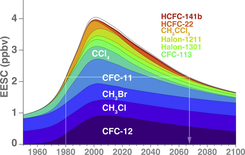
Effective equivalent stratospheric chlorine (EESC) versus year from 1950 to 2100 for a 5.2-year mean age-of-air (as in Newman et al., 2007), but using ODS levels from WMO (2014). These EESC values represent levels of chlorine that would be found over Antarctica. Brominated compounds are scaled by a factor of 60 to account for their greater ozone depletion efficiency with respect to chlorine. The contributions of the major ODSs to EESC are colored. The white lines show the EESC level in 1980, with an expected return to this 1980 level in about 2067.
The Montreal Protocol has not only reduced ozone depletion and started ozone layer recovery, but it has also protected climate because these ODSs are also powerful GHGs. For example, the 100-yr global warming potential (GWP) of CFC-12 is 10, 300 (WMO, 2014). Ramanathan (1975) first recognized that CFCs were powerful greenhouse gases and that their uncontrolled growth could accelerate climate change. Fig. 2 shows the radiative forcing of the primary ODSs controlled by the MP, as calculated from the observed and projected ODS levels along with the radiative efficiencies of the ODSs. While Fig. 1 shows that CFC-11 and CFC-12 make major contributions to ODS levels, Fig. 2 shows that they also collectively make a large contribution to global radiative forcing. These CFC forcings decline during the 21st century, but the growth of HCFC-22 (a transition compound) leads to a “plateauing” of the total Montreal Protocol ODS radiative forcing (i.e., compare to Fig. 1), with an overall decline beginning in the early-2020s.

Radiative forcing contributed by the major ODSs controlled under the Montreal Protocol as a function of year. The forcing is computed by taking observed (1950–2012) and projected (2013–2100) levels of ODSs (WMO, 2014), and then scaling by their radiative efficiencies.
CFC replacements were enabled by the use of transitional compounds such as hydro-chlorofluorocarbons (HCFCs). However, because they contained chlorine these HCFCs were eventually also controlled under the MP. These HCFC controls then spawned a transition to hydrofluorocarbons (HFCs). HFCs do not contain chlorine or bromine and therefore have only a small effect on ozone (UNEP, 2011). This small HFC effect on the ozone layer is indirect, caused by the HFC warming of the stratosphere (Hurwitz et al., 2015). Thus, the MP drove a transition from CFCs to HCFCs to HFCs. While the MP reduced ozone-depleting substance emissions, it created a situation where global HFC emissions were projected to increase total radiative forcing by fluorinated compounds, and this HFC increase would additionally add about 0.2 K of surface warming by 2050 (Velders et al., 2015). Fortunately, this increase was recognized by the Parties to the MP, and the Kigali Amendment was added to the MP in October 2016 to control HFCs.
3 Future of ozone science
The way forward for science begins with our first question. This is the “accountability” aspect, an aspect that has been in the science community for many years. Scientists predicted that ODSs would decline, and that ozone would start increasing as a result of that decline. Is this correct? Fig. 3 displays combined satellite data (black points) and coupled-chemistry model simulations (red points and smoothed line, Oman et al., 2016) of October total ozone images (upper panels) and the minimum Antarctic total ozone value for October (lower line plot). As shown in Fig. 1, Antarctic ozone tends to follow EESC, and total ozone levels will recover to 1980 ozone levels around 2070. A full return to 1960 levels will not occur until the 22nd century. The science challenge is to continue testing and improving the models (via data comparisons to hindcasts) that make these projections (accountability), and to identify knowledge gaps that impact these projections (new findings). The testing of models has been extensive performed by the science community (Eyring et al., 2005; SPARC, 2010) in order to ensure that these model projections can be trusted.

Upper panels show false-color images of October average total column ozone. The 1971 panel is derived from the NASA Nimbus-4 BUV instrument, and 2015 is from the NASA Aura satellite's Ozone Monitoring Instrument (KNMI. The 2041 and 2065 panels are from the NASA/GSFC GEOC-CCM model simulation. The lower panel shows each year's October average minimum (or lowest October average value) over Antarctica from satellite observations (black dots). The GEOSCCM model simulation shows that smoothed version of the red points (10-year Gaussian filter). Color scale is on the left-hand side. High ozone values are in red/yellow while low values are blue/purple.
At present, stratospheric ozone science is on a good foundation because of the observations available ‘and’ the adequate comparison with atmospheric models. Aircraft and satellite observations of a number of chemical species show that there are no major unknowns in stratospheric chemistry that might invalidate our current understanding–this contrasts with 1984, when (1) the major role of heterogeneous chemistry, and (2) the catalytic chlorine and bromine reactions (ClO + ClO and ClO + BrO) responsible for the Antarctic ozone hole were completely unknown. Furthermore, factors controlling ultraviolet and infrared fluxes are also well known.
A major question that remains concerning the recovery of Antarctic ozone levels involves our projections of ODSs. Fig. 1 shows the primary ODSs that contribute to EESC. These include CFC-11, CFC-12, and CCl4 (carbon tetrachloride or CTC). The problem with CTC is that in spite of being controlled under the Montreal Protocol, large CTC emissions have persisted (SPARC, 2016). These CTC emissions are likely a result of emissions from chloromethane (CH3Cl, CH2Cl2, CHCl3, and CCl4) production facilities and other more minor sources (Sherry et al., 2018). These additional CTC emissions (and other possible emissions) are not included in current projections; if they were they would lead to higher ODS levels in the stratosphere, with consequent later recovery dates. Recently, an increase of CFC-11 emissions has been observed in surface measurements, but reports to UNEP show that production and consumption of CFC-11 has declined to zero (Montzka et al., 2018). As of today, the cause of this CFC-11 emissions increase remains unknown. Atmospheric measurements that track ODS levels are part of a “compliance” aspect, insuring that countries adhere to both the letter of their commitments to the Montreal Protocol, but also to the spirit of the agreement to reduce ozone depletion.
The Merriam-Webster dictionary defines “vigilant” as “alertly watchful esp. to avoid danger.” This vigilance mainly focusses on paying close attention to the behavior of the ozone layer and to those ozone-depleting substances that can impact the ozone layer. While the primary long-lived ODSs (e.g., CFC-12, CFC-11, etc.) are controlled, there are many very short-lived (< 6 months) species (VSLS) that are not controlled because they were thought to not contribute significantly to stratospheric chlorine and bromine levels. However, research suggests that emissions of these short-lived species may contribute to stratospheric loading (Liang et al., 2017). Recent research suggests that some of these anthropogenic VSLS compounds could contribute if they are emitted in tropical regions where convective systems could carry them into the upper troposphere before they break down (Hossaini et al., 2017).
The biggest uncertainty in our future is the impact of the increasing primary greenhouse gases or GHGs (CO2, CH4, and N2O) or the stratospheric “climate” aspect. As noted above, ODS levels are now declining (Strahan and Douglass, 2018; WMO, 2014), and the stratosphere is showing some early signs that ozone has begun to recover. However, increasing GHGs are also modifying the ozone layer. Fig. 4 shows global total ozone changes from 1960 for observations (magenta crosses) and two model projections. The first simulation (black) is forced with observed and projected ODS levels from Fig. 1, but with an artificially fixed 1960 level of GHGs. The second simulation (black) is forced with both observed and projected ODS and GHG levels. Two points are noteworthy: first, the simulation forced by ODSs and GHGs (black line) is fairly consistent with the observations. Second, the omission of the increasing GHGs (green) lowers model values of stratospheric ozone by 2-3 DU before 1990 and by larger values after 1990. In other words, increasing GHGs elevate global ozone levels, and eventually lead to a much earlier recovery to 1960 levels.
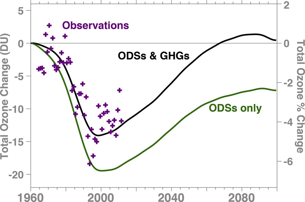
Total column ozone deviations from 1960 of the near global (60 °S–60 °N) annual averages. The simulations are from the GSFC 2-D model. The black line shows model total ozone forced with observed GHGs and ODSs up to 2012 and future GHG (> 2012) concentrations are based on the IPCC SRES A1B (medium) scenario. The dark green line shows model total ozone with GHGs artificially fixed to 1960 values. Ground-based total ozone observations (magenta crosses) are base-lined to the mid-1960s.
Because ODSs are declining (Fig. 1), the future levels of ozone will be controlled by the trajectories of the GHGs (Fig. 4) (WMO, 2014). These GHG trajectories currently constitute the largest uncertainty in the future of the ozone layer. Ozone layer sensitivity to GHGs results from two effects. First, as CO2 increases in the stratosphere, it leads to greater cooling of the stratosphere, slowing ozone loss, and causing ozone to increase mainly in the mid-to-upper stratosphere (Rosenfield et al., 2002). Second, increasing GHGs modify the wave dynamics of the stratosphere-troposphere system, speeding up the Brewer–Dobson circulation in the lower stratosphere. The increased lifting in the tropics acts to decrease tropical lower-stratospheric ozone, while increased sinking in the extra-tropics increases lower-stratospheric ozone in the extra-tropics (Li et al., 2009). The total impact of GHGs is to increase global ozone, with the largest ozone increases are in the mid-latitudes. The magnitude of the effects is dependent on the future levels of GHGs.
The atmospheric abundances of the primary GHGs (CO2, N2O, and CH4) have differing effects on the ozone layer (WMO, 2014). Increasing CO2 cools the stratosphere (as noted above) and it elevates global ozone. Both CH4 and N2O are source gases for stratospheric hydrogen and nitrogen, respectively. The increased N2O (by itself) is oxidized by O(1D) resulting in higher levels of reactive nitrogen, and therefore greater catalytic ozone loss (Crutzen, 1970).
Increased CH4 has a variety of effect (Brasseur and Solomon, 2005). CH4 is a sink for stratospheric chlorine (Cl + CH4 → HCl + CH3), but also a source of HOx that is involved with catalytic ozone loss. The overall effect of increasing CH4 elevates global ozone; while the overall effect of increasing N2O depletes global ozone. As noted above, these combined GHG increases ought to bring global total ozone back to a 1980 level by mid-century, earlier than recovery driven by the ODS decline alone (Fig. 4). Surprisingly, the Antarctic ozone hole is less sensitive to CO2, N2O, and CH4 abundances, and the hole ought to be recovered to 1980 levels in the 2070 time-frame (WMO, 2014).
The impact of GHGs on the stratosphere goes beyond just understanding their future pathways. Surface warming will increase the use of air conditioning and refrigeration technologies. Combined with growing populations in many developing countries, there will be greater demand for these technologies. This will in turn increase economic pressure to use efficient (and potentially ozone problematic) working fluids in these technologies. Further, ocean warming driven by GHGs has the potential to change the natural oceanic emissions of compounds containing chlorine and bromine (Yvon-Lewis et al., 2009).
Thus, while there are many things we understand about the impact of climate on the stratosphere, increasing GHGs to record levels truly leads us into “terra incognito”: the “unknown” aspect. Because tropospheric dynamics feeds energy and momentum to the stratosphere, minor changes in the troposphere could potentially drive large stratospheric changes. Transport and dynamics are weak points in our understanding because of the difficulty and non-linearity of forcing events on ozone such as the 2002 Southern Hemisphere major warming (Peters and Vargin, 2015) and the 2015–2017 QBO disruption (Newman et al., 2016; Osprey et al., 2016). The 2015-17 QBO disruption caused a major perturbation to stratospheric ozone with record low values in the Northern Hemisphere 2016 summer ozone levels (Tweedy et al., 2017). The 2002 major warming led to a record small Antarctic ozone hole (Stolarski et al., 2005). While these events are not necessarily caused by climate change, the inability to properly simulate them suggests gaps in our knowledge of tropospheric dynamical forcings of the stratosphere.
4 Conclusion
The way forward for MP science is contained in a number of areas. First, the science community must demonstrate accountability for their predictions of large ozone depletion from ODSs, and for projections of future ozone and the eventual recovery of the ozone layer. Second, vigilance must be maintained in the science community to both follow emerging threats to stratospheric ozone, and to also document compliance with the controls established by the Protocol. Third, increasing GHGs will be the dominant control of future ozone levels by the end of the 21st century (WMO, 2014). Some of these climate forcings are understood (e.g., cooling of the upper stratosphere), but unknowns remain, particularly with respect to minor tropospheric changes that could lead to major stratospheric changes.
Finally, scientific research must stay abreast of technology changes that could affect the stratosphere and be prepared to convey this new information to the MP. This objective effectively puts scientists in the roles of acting as authors of “environmental impact statements.” New rocket technologies and an accelerating annual launch rate is one area of concern, while developments in new stratospheric aircraft technologies should also be watched closely. In addition, because of climate change, there are now serious discussions about injecting particles into the stratosphere to reflect back to space incoming solar radiation. This solar radiation management, or geoengineering, needs to be carefully investigated in order to fully document how it impacts the stratospheric ozone layer.
Acknowledgements
This work was funded under a NASA Atmospheric Chemistry and Analysis Program grant: NNH10ZDA001N-ACMAP. Special thanks to Luke Oman, Eric Nash, and Eric Fleming for assistance with data and figures. I would also like to thank to Leslie Lait and Qing Liang for comments on the manuscript.