

1 Introduction
Tropical forests are an important contributor to the global carbon cycle since they encompass approximately 40% of the world's vegetation carbon stocks (Food and Agriculture Organization of the United Nations, 2010; Pan et al., 2011). Mapping the aboveground biomass (AGB) of tropical forests allows us to understand the spatial distribution of AGB, and repeated AGB mapping allows a better understanding of AGB dynamics (Feldpausch et al., 2004; Hughes et al., 2000; Lamlom and Savidge, 2003). Spatial remote sensing technology is the only operational solution for mapping AGB at regional and global scales since it provides data that cover large areas with a high spatial resolution and high revisit time.
Satellite optical, SAR (Synthetic Aperture Radar), and LiDAR data have widely been used for AGB mapping (Avitabile et al., 2016; Baccini et al., 2012, 2017; Labrière et al., 2018; Saatchi et al., 2011). In contrast to LiDAR data, optical images at low or medium resolutions and the SAR backscattering coefficient saturate at low to medium levels of AGB. Optical data allow AGB estimates until AGB levels between 55 and 159 t/ha, depending on the forest type (Lu et al., 2012; Zhao et al., 2016). SAR backscattering data in the L-band and P-band were mainly used to estimate the AGB. For Brazilian eucalyptus plantations, Baghdadi et al. (2015) found that the backscattering coefficient in the L-band (ALOS/PALSAR) saturates at an AGB of approximately 50 t/ha. For semiboreal forests in Sweden, Sandberg et al. (2011) report that the radar signal in the L-band saturates at 150 t/ha, whereas the radar signal in the P-band saturates at 290 t/ha. The arrival of the BIOMASS mission in 2021 (P-band) will allow the application of a tomographic technique on P-band SAR data for higher level AGB estimates (Le Toan et al., 2011; Reigber and Moreira, 2000). Minh et al. (2014, 2015, 2016) used the tomographic technique to compute P-band SAR backscattering coming from upper vegetation layers and then relate it to in situ forest AGB. The results showed that the P-band SAR signal from the upper vegetation layer is strongly correlated with forest AGB for AGB values ranging from 200 t/ha to 500 t/ha (Minh et al., 2014, 2016). This finding was the first demonstration that forest AGB can be estimated up to 500 t/ha with a 10% error at a 4-ha scale (Minh et al., 2015).
Currently, LiDAR is the only available technology able to estimate higher AGB. LiDAR measures the vertical structure of trees and allows precise tree height estimates until 40 m (Hilbert and Schmullius, 2012; Lefsky et al., 2005; Pang et al., 2008). The LiDAR-derived mean or median canopy height is strongly correlated with the trees AGB, with no saturation at higher AGB values (Lefsky et al., 2005; Mitchard et al., 2012; Saatchi et al., 2011). To date, the only free and open-access LiDAR data with a global coverage area are provided by the Geoscience Laser Altimeter System (GLAS) onboard the Ice Cloud and Land Elevation Satellite (ICESat). The arrival of the LiDAR data from the Global Ecosystem Dynamics Investigation (GEDI) in 2019 will allow better spatial coverage of the world's forest between 52°S and 52°N. The GEDI is composed of 3 lasers producing 10 parallel transects of observations. Each laser collects data in linear tracks of LiDAR shots with a 25-m footprint size and 60 m posting. The distance between each of the 10 transects is approximately 600 m (Patterson and Healey, 2015).
Several studies used mainly ground-based AGB, LiDAR and remote sensing data to map the AGB at the global and regional scales (Baccini et al., 2012; Saatchi et al., 2011; Vieilledent et al., 2016). Saatchi et al. (2011) and Baccini et al. (2012, 2017) used LiDAR data to obtain AGB estimates well distributed over different forests types. In the studies of Saatchi et al. (2011) and Baccini et al. (2012), the used methodologies can be summarized as follows: first, a model relating GLAS-derived metrics to in situ AGB was built and then applied to obtain GLAS-derived AGB estimates at each GLAS footprint location. Then, a model between GLAS-derived AGB and auxiliary variables (e.g., optical and SAR images and environmental maps) is built. Finally, this model is applied to the auxiliary variables to map the AGB. Vieilledent et al. (2016) used a dense field inventory (1771 plots) well distributed in space and remote sensing and climatic variables to map the AGB in Madagascar. First, a random forest (RF) model was used to relate in situ AGB to the MODIS (Moderate Resolution Imaging Spectroradiometer) EVI (Enhanced Vegetation Index) and percent tree cover, parameters derived from the SRTM digital elevation model, and climatic variables. Then, this calibrated random forest model was applied to map the AGB of forested areas in Madagascar.
The use of optical and SAR amplitudes from remote sensing data, which saturate at medium to low AGB values (lower than 150 t/ha for L-band), as predictive variables for AGB mapping leads to an underestimation of high AGB values (Lu et al., 2012; Vieilledent et al., 2016; Zhao et al., 2016). To overcome such a saturation issue, El Hajj et al. (2017) and. Fayad et al. (2016) used the Regression Kriging (RK) method (Hengl et al., 2004). First, a semivariogram of the residuals, the difference between AGB map obtained from the auxiliary variables (e.g., remote sensing, environment and climatic data) and GLAS-derived AGB, was adjusted. Then, semivariogram parameters were used to perform an ordinary kriging interpolation of residuals and provide a map of residuals. Finally, the residuals map was added to the AGB map obtained from the auxiliary variables (remote sensing, environment and climatic data) to improve the estimation of high AGB values.
The main goal of this study is to map the AGB in Gabon forests. First, an RF model that relates remote sensing (RS) variables to AGB values extracted from reference AGB maps was adjusted. Then, the calibrated RF model was applied to remote sensing data to produce an AGB map of Gabon. To improve the accuracy of the remote sensing-derived AGB map, the GLAS LiDAR data were considered. First, the GLAS data were calibrated to AGB, providing a spatially distributed (GLAS footprints geolocation) GLAS-derived AGB (surrogate AGB data). Second, the spatial dependency between residuals (RS-derived AGB map – surrogate AGB data at each GLAS footprint location) was modeled by mean of a semivariogram. Then, the semivariogram parameters were used to perform a regression kriging (RK) interpolation of residuals, providing a residual map. Finally, the residual map was added to the RS-derived AGB map. A description of the study area and the datasets is given in Section 2. Section 3 presents the methodology. The results and discussion are shown in Sections 4 and 5, respectively. Finally, Section 6 presents the conclusions.
2 Study area and dataset
2.1 Study area
Gabon has an area of ∼270,000 km2 and is located on the equator on the west coast of Central Africa. According to the World Bank open data website (https://data.worldbank.org/), the forested area in Gabon represented ∼89% Gabon's area in 2015. The climate is equatorial, with a fairly high humidity (85–100% in the rainy season). Near the coast, the climate is more temperate because of the marine winds. Temperatures range from 21 °C in the southwest to 27 °C on the coast and inland.
2.2 Datasets
2.2.1 Reference AGB maps
In this study, 50-m AGB maps for four regions of the AfriSAR campaign (namely, Lopé, Mabounie, Mondah, and Rabi (Hajnsek et al., 2016)) were used as the reference AGB dataset to calibrate and validate the result of our AGB mapping (Fig. 1). These maps (total area of 340 km2) were generated by Labrière et al. (2018) using small-footprint airborne LiDAR data (acquired in 2007 for Manounie, 2011 for Mondah and 2015 for both Lopé and Rabi). A simple power-law model relating field-based AGB to the median canopy height (LiDAR-derived metrics that performed better than mean canopy height) was built. The calibrated model was then applied to derive the AGB maps for the four regions. For the four Gabonese regions, the values of the RMSE on AGB estimates at 100-m and 50-m spatial resolutions were 47.5 t/ha and 77.0 t/ha, respectively.
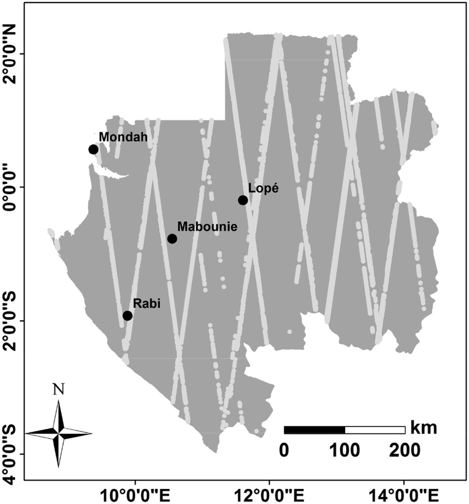
Country of Gabon. Black points represent the location of the four reference AGB maps. The gray points correspond to GLAS footprints.
2.2.2 ALOS/PALSAR data
A 25-m mosaic SAR image in the L-band acquired by the Phased Array Synthetic Aperture Radar (PALSAR) onboard the Advanced Land Observing Satellite (ALOS) was used. The mosaic SAR is dual-polarization (HH and VH). Only the VH polarization was used since it is more sensitive to forest layers than HH (Minh et al., 2014). An L-band SAR image in VH polarization was calibrated to obtain the gamma naught backscattering coefficient:
| (1) |
The original 25-m resolution map was resampled to 50 m (using the mean as the resampling method). Height GLCM (Gray-Level Co-Occurrence Matrix) texture indices were calculated using a 3 × 3 window on the resampled image: mean (SAR_Mean), variance (SAR_Var), homogeneity (SAR_Hom) contrast (SAR_Cont), dissimilarity (SAR_Diss), entropy (SAR_Ent), second moment (SAR_SecM), and correlation (SAR_Corr).
2.2.3 Optical data
In this study, the MODIS EVI product for the year 2010 was used. EVI images have a spatial resolution of 250 m and a revisit time of 16 days. From the 2010 EVI time series, minimum (MIN_EVI), mean (MEAN_EVI) and maximum (MAX_EVI) EVI values were computed, as well as the first seven principal components issued from the principal component analysis of the EVI time series (PC1, PC2, …, PC7). In addition, as for the SAR image, eight GLCM texture indices were calculated using 3 × 3 windows on the MEAN_EVI. The 8 GLCM texture indices were Mean (EVI_Mean), Variance (EVI_Var), Homogeneity (EVI_Hom), Contrast (EVI_Cont), Dissimilarity (EVI_Diss), Entropy (EVI_Ent), Second moment (EVI_SecM), Correlation (EVI_Corr). All EVI-derived layers were resampled to a 50-m resolution.
2.2.4 Digital elevation model data
A Digital Elevation Model (DEM) with a spatial resolution of 30 m was obtained from the Shuttle Radar Topography Mission (SRTM). Four variables were derived from the SRTM DEM: elevation (Elev), slope (θ), terrain index (TI), surface roughness (Roug), and height above nearest drainage (Nobre et al., 2011) (Hand). The TI map was obtained by calculating the difference between the highest and lowest elevations in a 3 × 3 moving window. The surface roughness map was obtained by computing the standard deviation of the elevation in a 3 × 3 moving window. All SRTM-derived variables (θ, TI, Roug, and Hand) were resampled to 50 m using the mean as the resampling method.
2.2.5 Average rainfall map
The rainfall data were obtained from NASA's tropical rainfall measuring mission (TRMM). TRMM data are recorded daily with a spatial resolution of ∼25 km. The average rainfall map was computed by averaging daily TRMM rainfall between 2003 and 2013. The average rainfall map was resampled to 50 m. Rainfall was used in AGB mapping because of the strong relationship between precipitation and biomass (Silvertown et al., 1994; Yan et al., 2015). In this study, the average rainfall variable is referred to as “Prec”.
2.2.6 Land cover maps
Four land cover maps were used in this study to mask out non-forested areas: (1) three ALOS/PALASR forest/non-forest products with a spatial resolution of 25 m for the years of 2007, 2010, and 2015 (http://www.eorc.jaxa.jp/ALOS/en/palsar_fnf/fnf_index.htm), and (2) one ESA (European Space Agency) land cover product with a spatial resolution of 20 m derived from Sentinel-2 images for the year 2016 (https://www.esa-landcover-cci.org/). These four land cover maps are the only available maps at dates close to those of the reference AGB maps (2007, 2011, and 2015).
2.2.7 Spaceborne ICESat/GLAS LiDAR data
In this study, we used satellite LiDAR data that were acquired between 2003 and 2009 by the GLAS sensor onboard the ICESat Satellite. GLAS is a laser sensor operating in the near-infrared wavelength (1064 nm). It illuminates nearly circular footprints with a diameter of approximately 70 m. Spacing between two consecutive footprints in the along-track direction is approximately 172 m. The horizontal geolocation accuracy of the GLAS footprints is 3.7 m (on average) (Carabajal and Harding, 2006; Huang et al., 2011). In this study, only the Level-1A altimetry data (GLA01) and Level-2A (GLA14) products available from GLAS were considered. The GLA01 data include transmitted and received waveforms from the GLAS sensor. The GLA14 data are derived from the GLA01 product and include several useful data for each footprint, such as the cloud flag index, saturation waveform index, land surface elevation from SRTM, centroid elevation derived from the waveform, and background noise.
Several filters were applied to eliminate unreliable GLAS data (i.e. data affected by atmospheric conditions). Variables used for filtering were provided by the GLA14 product. A footprint was removed if: (1) the GLAS-derived centroid elevation is significantly different from that obtained from SRTM (|GLAS − SRTM| > 100 m); (2) the associated waveform has a low signal-to-noise ratio (SNR) (SNR < 15) (Carabajal and Harding, 2006); (3) the associated saturation index indicated a saturated waveform (saturation index satNdx different from 0); and (4) a cloud is present (cloud flag FRir_qaFlag different from 15). In addition, an ALOS/PALSAR-derived forest-non-forest mask for the year 2010 was used to eliminate GLAS footprints located outside forest stands. A total of 33,275 reliable GLAS footprints were located in forested areas (density of 0.13 footprint/km2 across Gabon).
Moreover, metrics were derived from reliable GLAS waveforms provided in the GLA01 product to represent the vertical structure of the canopy. These metrics are as follows.
- (1) Waveform extent (Wext): a noise threshold equal to 4.5 times the standard deviation of the background noise was used to determine the beginning and end of the waveform (Lefsky et al., 2007). The waveform extent is the difference between the signal end and signal start.
- (2) Percentile heights (H) of GLAS waveforms: in this study, the first Gaussian peak was considered the canopy's top peak, and the stronger of the last two Gaussian peaks was selected as the ground peak (Rosette et al., 2008). After identifying the canopy's top and ground peaks, the percentile heights of the GLAS waveforms (10 through 90%) were calculated from the signal's beginning (Fayad et al., 2016).
- (3) Leading Edge (LE): the elevation difference between the signal start and the canopy's peak's center (Hilbert and Schmullius, 2012).
- (4) Trailing Edge (TE): the difference between the signal end and the ground peak's center (Hilbert and Schmullius, 2012).
3 Methodology
Our methodology to map AGB consisted of two main steps (Fig. 2). In the first step, an RF model that relates reference AGB to significant RS variables was calibrated. Then, this calibrated model is applied to produce an RS-derived AGB map with a 50-m spatial resolution. The resampling to 50 m of RS data (ALOS/PALSAR, SRTM, EVI, Precipitation) was performed in order to have RS data with the same spatial resolution as the reference AGB maps. In the second step, the contribution of GLAS-derived AGB (surrogate AGB data) to improve the RS-derived AGB map was investigated. First, the best regression between GLAS waveform-derived metrics and a reference AGB was built. Then, we tried to improve the RS-derived AGB map by adding the kriged residuals (RS-derived AGB map – surrogate AGB data) to the AGB map from the first step (El Hajj et al., 2017; Fayad et al., 2016).
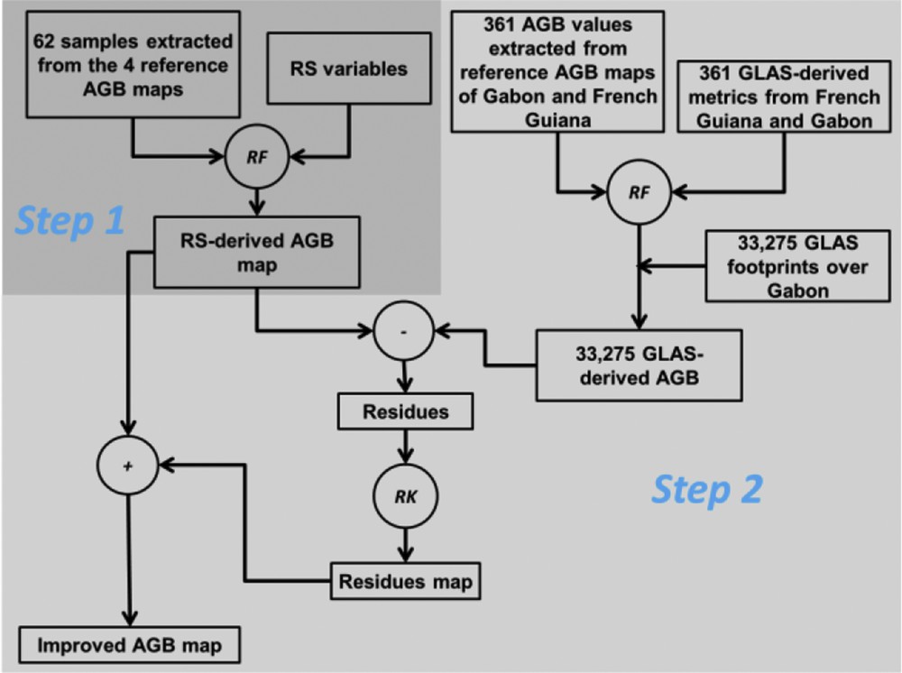
Procedure for AGB mapping.
Over Gabon, GLAS footprints cover only the Mondah region with low (<150 t/ha) AGB values. Therefore, these footprints are not sufficient to build a robust model that relates GLAS-derived metrics to AGB in very dense forests, where AGB can reach up to 600 t/ha. To overcome such limitations, GLAS data available over French Guiana and the AGB map created by Fayad et al. (2016) for French Guiana were used. This AGB map (resolution of 1 km) was elaborated using airborne LiDAR, spatial LiDAR (GLAS), SAR, optical and environmental data, with an accuracy of 50.2 t/ha (Fayad et al., 2016).
Labrière et al. (2018) reported that site-specific models built between AGB and airborne LiDAR-derived metrics for each of two regions in French Guiana and four regions in Gabon give similar AGB estimates as the model developed using data from all these regions together. Thus, the model built using GLAS data and reference AGB available over French Guiana and Gabon is suitable to predict AGB across Gabon at the landscape scale (Labrière et al., 2018).
3.1 Mapping wall-to-wall AGB
To map the AGB, first, 62 samples were drawn on the Gabon reference AGB maps in such a way as to delimit homogenous AGB pixels values (standard deviation lower than 50 t/ha). The 62 samples cover between 8 and 20 pixels of the reference AGB maps and they are taken from the four regions (Lopé, Mabounie, Rabi, and Mondah). The AGB value associated with each sample is the mean of AGB pixels values that the sample covers. These mean values cover the range of AGB values majority encountered in the four regions. Then, the mean of all RS variables were calculated for each of the samples. Third, an RF model that relates the mean AGB of samples to all auxiliary RS variables was adjusted. Fourth, the more significant RS variables were selected, and the RF model was readjusted using only these significant RS variables. The determination of significant variables was conducted by using the increase in the mean square error of the predictions (%IncMSE). Finally, the readjusted RF model was applied to significant RS variables, and an AGB map with a 50-m spatial resolution was obtained.
The RS-derived AGB map was compared to the Gabon reference AGB maps to assess its accuracy. For each reference AGB map, a grid composed of meshes with the size of 200 m × 200 m (16 pixels) was created, and the mean AGB was calculated for each mesh. Then, the mean AGB-values of the reference AGB maps and the AGB-values from the RS-derived AGB map were compared. Meshes containing the 62 samples used to build the RF model were not used to validate the RS-derived AGB map. This procedure was conducted for the 4 airborne-derived reference AGB maps. Finally, the mean values of the RS-derived AGB map and the mean values of reference AGB maps were compared through the Root Mean Square Error (RMSE), bias, and Pearson correlation coefficient (R2).
The RS-derived AGB map refers to the year 2010 since the used SAR and optical RS variables were acquired in 2010. However, the reference AGB maps refer to the years 2007 (Mabounie), 2011 (Mondah), and 2015 (Lopé and Rabi). Four forest/non-forest maps were considered in the validation of the RS-derived AGB map. These maps correspond to ALOS/PALSAR forest/non-forest products for the years of 2007, 2010 (the map for 2011 is not available) and 2015, as well as to the Sentinel-2 land cover product for 2016 (only this year is available). For the years 2015–2016, it was difficult to choose between the ALOS-derived map and the one based on Sentinel-2 data since the analysis of these two products by photointerpretation showed some artifacts. Therefore, to avoid the use of misclassified pixels (forest/non-forest), meshes were eliminated in the validation of the RS-derived AGB map if they contained at least one deforested pixel in the four forest/non-forest maps used in this study. The application of this criterion allows the elimination of 1557 meshes on from a total of 8472 meshes used to validate the AGB map. For non-deforested areas, we hypothesize that the AGB was not considerably changed.
3.2 ICESat/GLAS surrogate AGB data
A RF model that relates the reference AGB from Gabon and French Guiana to GLAS-derived metrics was first built to relate the reference AGB to the GLAS metrics (Wext, LE, TE, H10 through H90 with a 10% step) and DEM variables (slope, TI, and Roug). The database used to build the RF model comprises 68 samples from Gabon and 293 samples from French Guiana. Then, the significant predictive variables were determined based on the %IncMSE. Finally, the RF model was readjusted using only the significant GLAS metrics and DEM variables and applied to obtain the surrogate AGB data, which are AGB values for the 33,275 GLAS footprints throughout forested areas in Gabon.
3.3 Improving the RS-derived AGB map
The contribution of surrogate AGB data through the regression kriging (RK) interpolation technique to improve the RS-derived AGB was investigated in this study (El Hajj et al., 2017; Fayad et al., 2016). Kriging allows the interpolation of residuals, resulting from the difference between RS-derived AGB and surrogate AGB data at each GLAS footprint location. The kriging results from an omnidirectional semivariogram model were inferred from residuals data. The semivariogram describes the spatial dependency between residuals and draws the semivariance as a function of the distance between residual pairs using the following function:
| (2) |
After drawing the empirical semivariogram, an admissible model is fitted to the empirical variogram, determining the semivariogram function parameters. At any spatial location , the RK estimation (known as a Best Linear Unbiased Estimator) is performed using the fitted semivariogram according to the linear equation:
| (3) |
Accordingly, the semivariogram of residuals (RS- derived AGB – surrogate AGB at each GLAS footprint locations) was computed (distance h with a step of 3000 m), and the RK interpolation of residuals was performed to create a gridded residual map. Finally, the RS-derived AGB map and the residuals map are added (RK method) for the potential to improve the obtained RS-derived AGB map.
3.4 Comparing to existing AGB maps
The precision of the final AGB map was compared to that of the most recent and accurate pan-tropical AGB map produced by Avitabile et al. (2016) (Avitabile's AGB map). Avitabile's AGB map represents the AGB values in African forested areas for the period 2007–2008 (Avitabile et al., 2016). Avitabile et al. (2016) developed a fusion model based on the use of ground-based AGB data to combine the global AGB maps of Saatchi et al. (2011) and Baccini et al. (2012) into a pan-tropical AGB map (1 km resolution). The fusion model consists of bias removal and weighted linear averaging of both the Saatchi et al. (2011) and Baccini et al. (2012) AGB maps to produce an AGB map with higher accuracy. Avitabile's AGB map has a spatial resolution of 1 km, whereas our reference AGB maps have a spatial resolution of 50 m. The accuracy of Avitabile's AGB map was computed using our reference AGB maps; first, each set of AGB pixels from our reference AGB maps that fall within each grid of Avitabile's AGB map were averaged. Then, the pixel values from Avitabile's AGB map were compared to the averaged pixel values from the reference AGB maps using statistical indices (bias, RMSE, and R2).
Moreover, we compared the accuracy of our final AGB map and that of the high-resolution (30 m) AGB map produced by Baccini et al. (2017) for the year 2000 (Baccini's AGB map). Baccini's AGB map was derived using mainly GLAS-derived metrics and Landsat data for the year 2000. The accuracy of Baccini's AGB map was computed using our Gabon reference AGB maps following the same evaluation procedure described in Section 3.1.
4 Results
4.1 Mapping wall-to-wall AGB
The 62 samples extracted from the 4 Gabon reference AGB maps are related to the RS variables through the RF model. The significant RS variables that contributed the most to the estimation of AGB were determined by using the increase in the mean square error of the predictions (%IncMSE > 3.5). The use of %IncMSE >3.5 allows reducing the number of predictive variables while keeping accurate the estimation of AGB. The results showed that the significant variables are SAR_Mean, Elev, Hand, TI, Roug, θ, Prec, EVI_max, and PCA1 (Fig. 3). This finding is in line with the results obtained by Fayad et al. (2016).
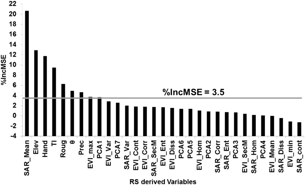
Variables' order of importance for the estimation of reference AGB of Gabon and the French Guiana. The gray horizontal line represents the level of %IncMSE of 3.5.
The RF model estimates the reference AGB samples from significant variables with an R2 of 0.96, an RMSE of 38.6 t/ha, and a bias of 2.1 t/ha (Fig. 4). The calibrated RF model highly overestimates the AGB for AGB values lower than 100 t/ha because the radar wave in the L-band (1.27 GHz) penetrates the vegetation cover, reaches the ground, and generates a backscattered signal with a significant contribution of the soil in addition to the vegetation's contribution.
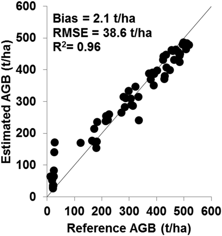
RS-derived AGB against Gabon reference AGB.
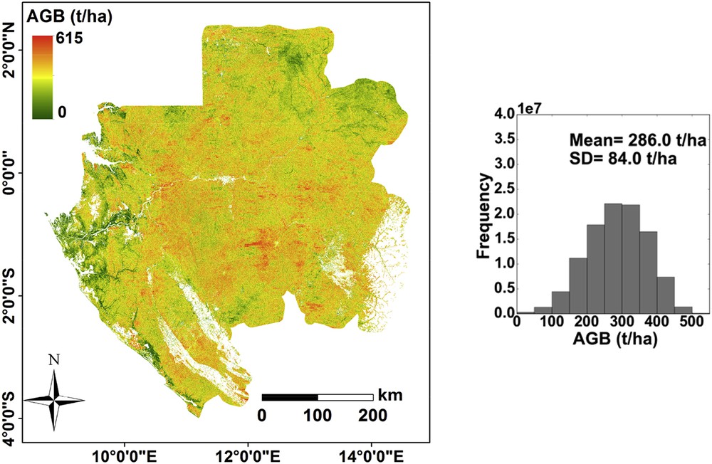
The RF is applied on the significant RS variables, and an AGB map was obtained (Fig. 5). The AGB values range from 50 to 500 t/ha. The mean AGB value is 315.6 t/ha, and the standard deviation (SD) is 82.2 t/ha.

RS-derived AGB map.
4.2 Accuracy of the RS-derived AGB map
For all reference AGB values, the comparison between RS-derived AGB and reference AGB values averaged over meshes with a size of 200 m × 200 m yields an RMSE of 63.3 t/ha, a bias of 19.1 t/ha, and a R2 of 0.53 (Fig. 6). In addition, statistics were calculated separately for reference AGB values lower and higher than 100 t/ha. For AGB values lower than 100 t/ha, the results showed that the RS-derived AGB values overestimate the reference AGB (bias = 89.8 t/ha), with an RMSE of 102.0 t/ha. For AGB higher than 100 t/ha, the RS-derived AGB slightly overestimates the reference AGB values by 15.4 t/ha (RMSE = 60.5 t/ha).
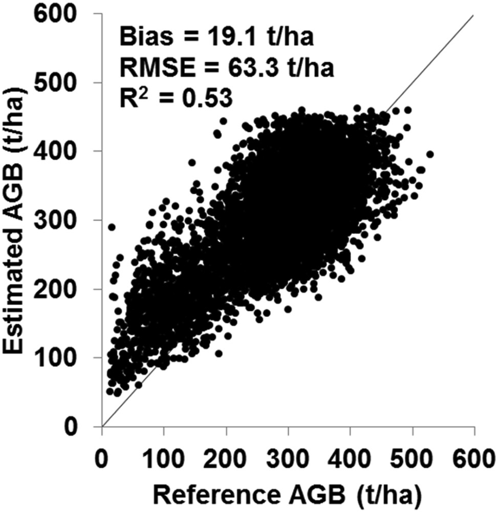
RS-derived AGB against the reference AGB map for the four Gabonese regions. Each point represents averaged AGB pixels values on a mesh of 200 m × 200 m (16 pixels).
4.3 ICESat/GLAS surrogate AGB data
Three hundred and six GLAS footprints located in French Guiana and 55 footprints located in Gabon as well as reference AGB values were used to build an RF model that relates AGB values to GLAS-derive metrics and DEM variables (θ, TI, Roug). The results show that Wext, LE, TE, H10, θ, and TI are the most significant predictive variables for AGB estimates. From these significant variables, the RF allow AGB estimates with good accuracy (RMSE = 25.9 t/ha, bias = −0.1 t/ha and R2 = 0.96) (Fig. 7). Moreover, the accuracy on AGB estimates was computed separately for AGB reference data from Gabon and French Guiana. The RMSE is 30.9 t/ha (bias = 19.5 t/ha) over Gabon and 24.9 t/ha (bias = −3.6 t/ha) over French Guiana. The calibrated AGB was applied to estimate the AGB from the 33,275 GLAS footprints of forested areas in Gabon.
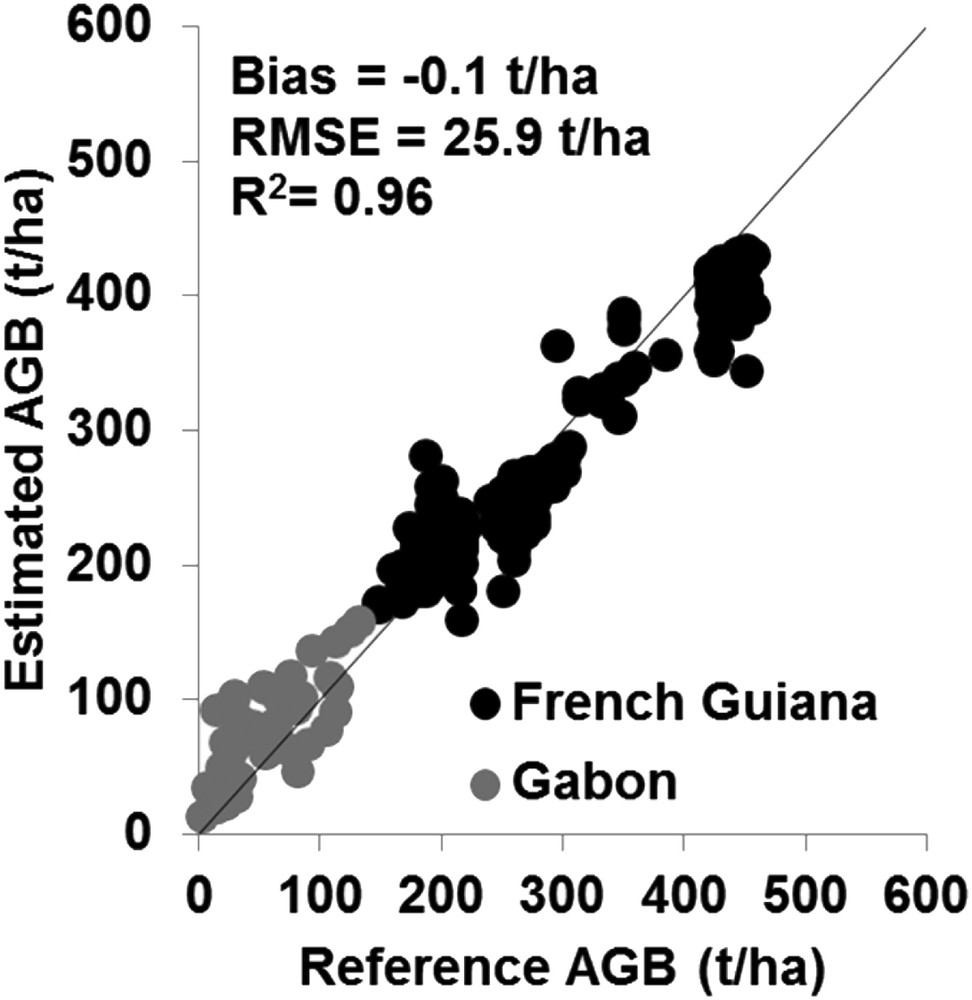
GLAS-derived AGB against the reference AGB from Gabon and the French Guiana.
4.4 Improving the RS-derived AGB map
For a possible improvement in the RS-derived AGB map using the regression kriging (RK) technique, the semivariogram of residuals was estimated and modeled. First, the difference between the RS-derived AGB map and the GLAS surrogate AGB data was computed at the location of each GLAS footprint. Then, the semivariance of the residuals was computed. Fig. 8 shows the semivariogram estimation at distances ranging from zero to 300,000 m (gray points), corresponding to the local semivariance at the extent of Gabon. Later, the semivariance was fitted using two functions, one exponential and one Gaussian. For the exponential function, the partial sill is 992 (t/ha)2 and the range was 3950 (m). For the Gaussian function, the partial sill is 762 (t/ha)2 and the range is 256,050 m (Fig. 8). Semivariance parameters are used to interpolate residuals and obtain a residual map. Later, the RS-derived AGB map and the residual maps were summed to obtain the final AGB map (Fig. 10).
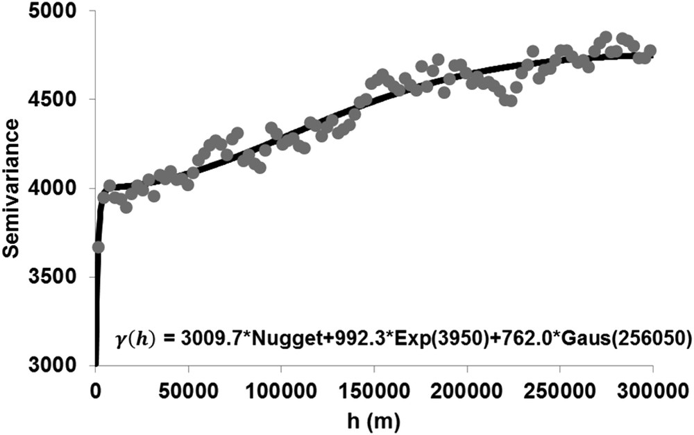
Semivariogram of the residuals. Nugget = 3009 (t/ha)2.
Final AGB map over Gabon.
In addition, the kriging error standard deviation map resulting from the regression kriging of the difference between RS-derived AGB and GLAS-derived AGB was also obtained. This map was added to the spatially homogeneous residual standard deviation resulting from the regression of reference AGB with GLAS metrics (Fig. 7) to obtain the kriging uncertainty map (Fig. 9). Fig. 9 shows that uncertainty low values (about 50 t/ha) are concentrated around GLAS footprints and increase as moving away from GLAS footprint positions to reach 79 t/ha. The kriging uncertainty map reflects the uncertainty on the final AGB map (Fig. 10) resulting from the complex mapping process that mixes GLAS, RS variables, and scarce AGB data.
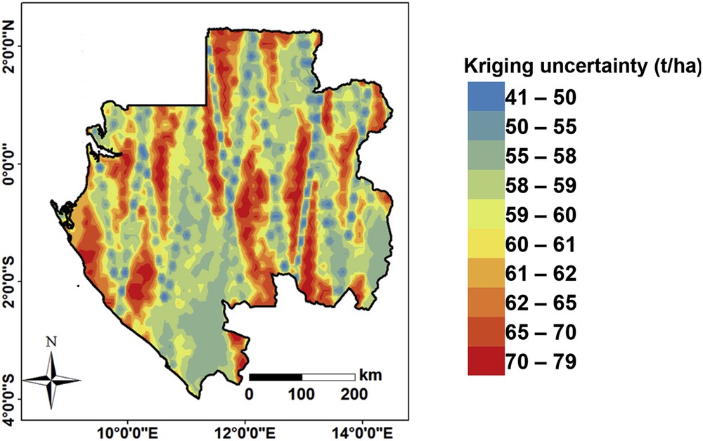
Kriging uncertainty map.
The feasibility of the RK method to improve the RS-derived AGB map was assessed by analyzing the evolution in the accuracy of the RS-derived AGB map after adding the residuals’ map. For the RS-derived AGB map, the precision of the final AGB map was calculated using meshes with a dimension 200 m × 200 m. For all AGB values, the result shows that the final AGB map has an accuracy of 70.2 t/ha (bias = 18.2 t/ha) (Fig. 11). For AGB values lower than 100 t/ha, the final AGB map overestimates the reference AGB values by 75.9 t/ha (RMSE = 92.1 t/ha). For reference AGB values higher than 100 t/ha, the final AGB map slightly overestimates the reference AGB values by 15.2 t/ha (RMSE = 68.8 t/ha). Accordingly, the integration of GLAS surrogate AGB data through the RK method slightly improves the accuracy of AGB estimates only for AGB values < 100 t/ha. Indeed, the final AGB map overestimates the AGB less (bias = 75.9 t/ha) than the RS-derived AGB map (bias = 89.8 t/ha). Moreover, the integration of GLAS surrogate data decreased the RMSE on AGB estimates by 9.9 t/ha for AGB values lower than 100 t/ha; the RMSE of the final AGB map is 92.1 t/ha compared to 102.0 t/ha for the RS-derived AGB map. For AGB values higher than 100 t/ha, the results show that the integration of surrogate AGB data does not improve the accuracy of the RS-derived AGB map; the RMSE of the final AGB map was 68.8 t/ha, compared to 60.5 t/ha for the RS-derived AGB map. Ground-based AGB produced at 1 ha (Labrière et al., 2018) were used to validate the accuracy of the final AGB map. Results showed that the final AGB map estimates the 1-ha ground-based AGB (57 samples) with an RMSE of 102.5 t/ha. The final AGB map is available from the French Land Data Center (https://www.theia-land.fr/en).
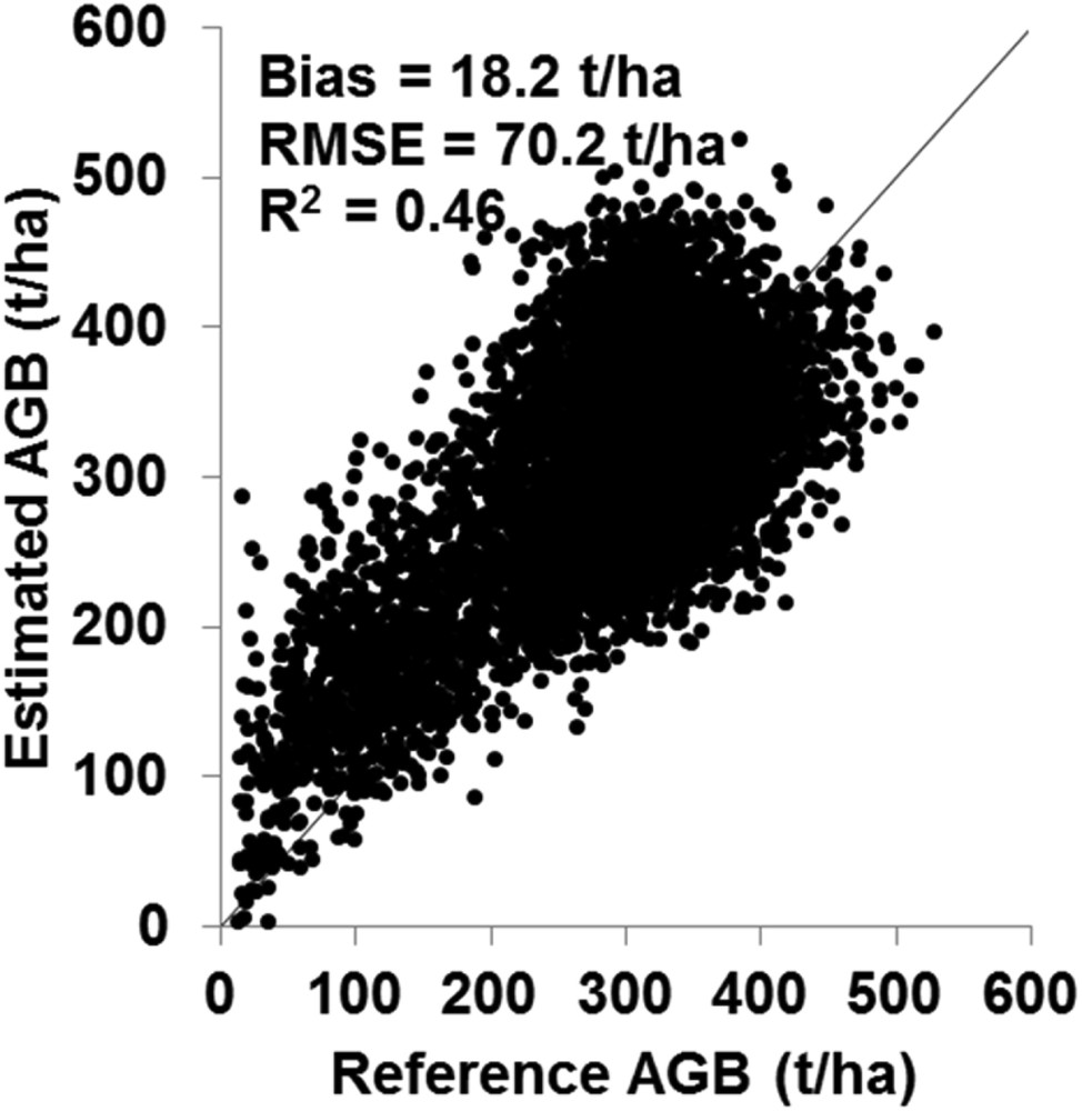
Final AGB map against the reference AGB map for the four Gabonese regions. Each point represents averaged AGB pixels values on a mesh of 200 m × 200 m (16 pixels).
4.5 Comparison between the RS-derived AGB map and existing AGB maps
The accuracy of our final AGB map was compared to that of Avitabile's AGB map (Avitabile et al., 2016). The results show that the accuracy of the Avitabile's AGB map (RMSE = 114 t/ha bias = 51.2 and R2 = 0.01) is much lower than that of our RS-derived AGB map (Figs. 6 and 12). Moreover, the precision of our final AGB map was compared to that of Baccini's high-resolution AGB map for the year 2000 (Fig. 13). For our final AGB map, the reference AGB maps of the 4 regions of Gabon were used to evaluate the accuracy of Baccini's AGB map using mean values computed on meshes of 200 m × 200 m. The results show that the Baccini's AGB map has an accuracy of 92.1 t/ha (bias = 33.2 and R2 = 0.06), which is lower than the accuracy of our RS-derived AGB map (Fig. 13). Particularly, Baccini's AGB map highly overestimates (bias = 208.7 t/ha, RMSE = 212.9 t/ha) the AGB for reference AGB values lower than 100 t/ha.
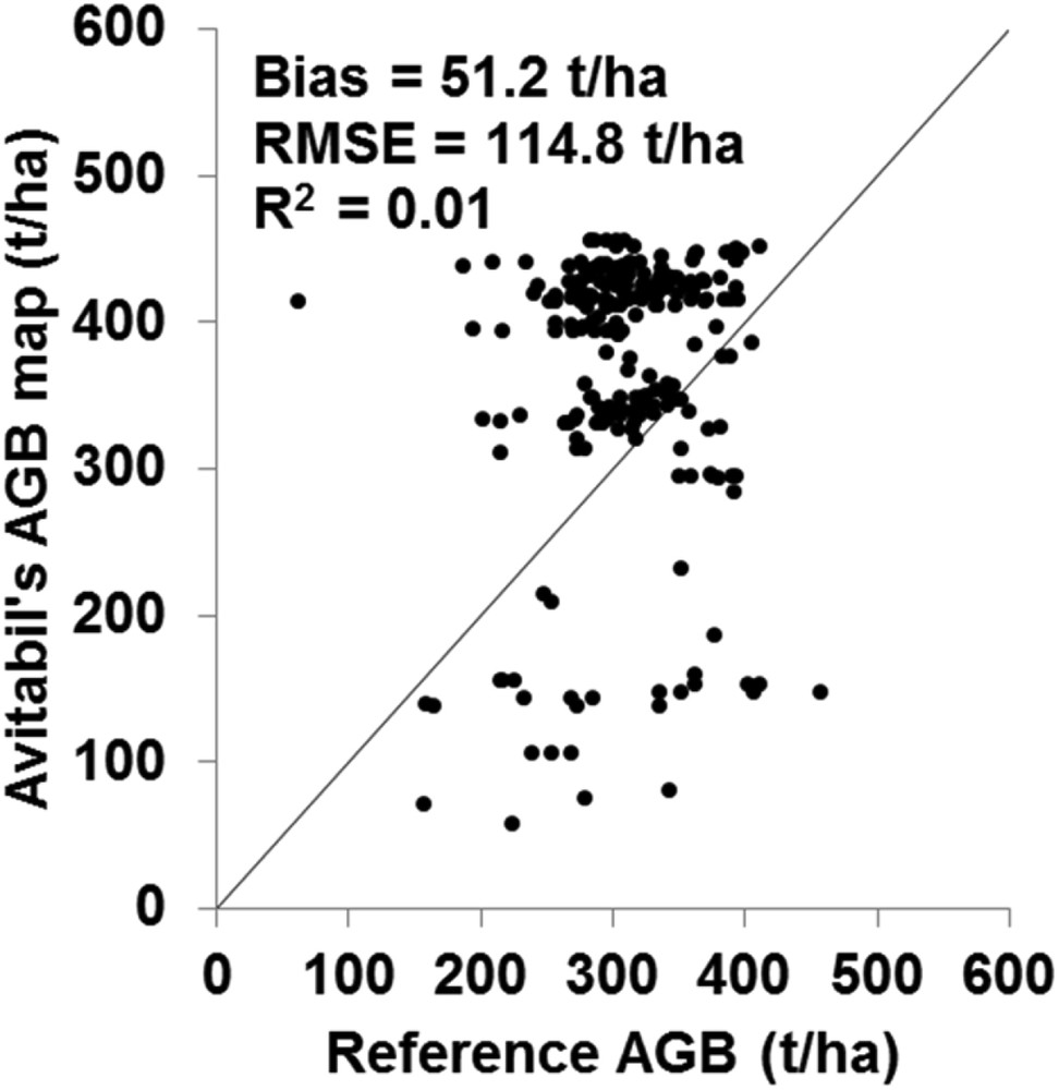
Avitabile's AGB map against the reference AGB maps of the four Gabonese regions.
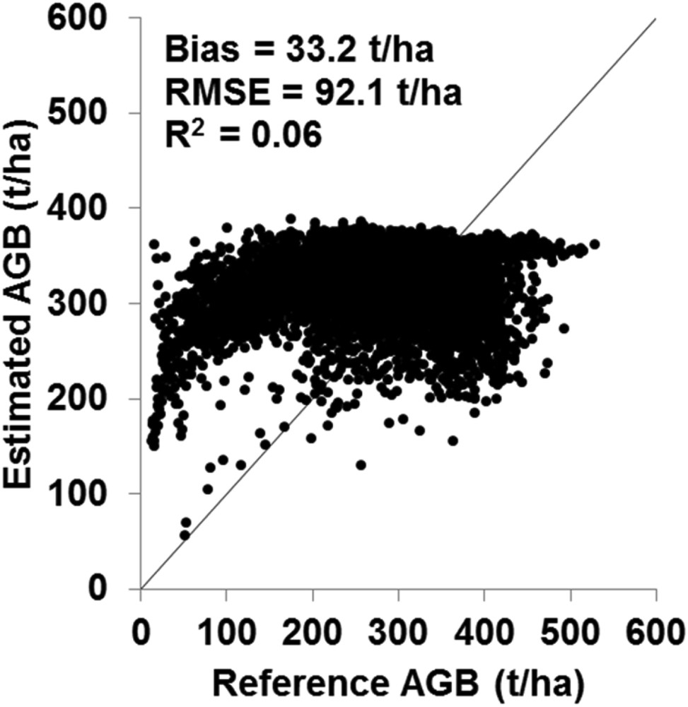
Baccini's AGB map against the reference AGB maps of the four Gabonese regions.
5 Discussion
This study aimed to produce an AGB map for the forested areas in Gabon in 2010. Four reference AGB maps were used to calibrate RS variables to AGB through an RF model. From the RS variables, the most significant predictive variables were the mean of L-band backscattering in VH polarization and the DEM-derived variables (Elev, Hand, TI, Roug, θ). This was expected, since the VH polarization represents the volume scattering and is sensitive to the tree cover. In a recent study, Minh et al. (2018) showed that the ALOS/PALSAR backscattering in VH polarization depends strongly on the AGB of Madagascar forested areas until an AGB of 150 t/ha. In addition, the dependency between DEM-derived variables and AGB was reported in several studies (Fayad et al., 2016; Silvertown et al., 1994; Vieilledent et al., 2016; Yan et al., 2015).
The obtained RS-derived AGB map tends to highly overestimate (89.8 t/ha) the reference AGB for a reference AGB lower than 100 t/ha (Fig. 6). To understand this overestimation, a photointerpretation was performed using optical images. The photo-interpretation reveals that the overestimation of low AGB values (AGB < 100 t/ha) occurred mainly in areas with weakly dense trees (examples shown in Fig. 14). For these areas, it seems that both ground and vegetation parameters contribute to the total backscatter signal in the L-band. Thus, the ALOS/PALSAR backscattered signal does not only depend on the tree cover; it also contains an additive contribution from the ground. This ground additive contribution on the L-band SAR backscattering coefficient (the most significant RS variables in the RF model) induces an overestimation of the RS-derived AGB. The accuracy of the RS-derived AGB map was good, with an RMSE of 60.5 t/ha (bias = 15.4 t/ha) for a reference AGB higher than 100 t/ha.
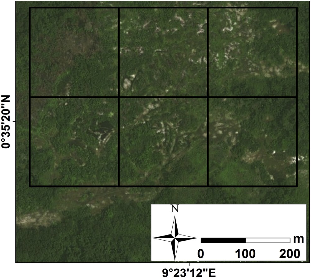
Meshes (black squares with a dimension of 200 m × 200 m), where a high overestimation of AGB values were obtained in our final map. The green color represents the forest cover, white and brown colors represent the bare soils.
In this study, we aimed to improve the RS-derived AGB maps using LiDAR-derived AGB values along with the RK interpolation technique. The results showed that the integration of GLAS surrogate AGB data helps reduce the overestimation of AGB estimates for AGB values lower than 100 t/ha. However, the RK slightly improves the AGB estimates for AGB higher than 100 t/ha. This is mainly due to the low density of GLAS data over forested areas in Gabon (0.13 footprints/km2).
The results showed that the accuracy of our final AGB map was much better than that of the most recent accurate pan-tropical map produced by Avitabile et al. (2016). There are two possible reasons. First, the backscattering coefficients in the L-band were not considered as a predictive variable to estimate the AGB values of the input maps to the fusion method (maps used to generate Avitabile's AGB map) (Avitabile et al., 2016). Second, the reference AGB value used in the study of Avitabile et al. (2016) are issued from different regions with forest types and structures different from those of forested areas in Gabon (El Hajj et al., 2017). The above reasons could also explain the lower accuracy of Baccini's AGB map (Baccini et al., 2017) in comparison to our RS-derived AGB map. Moreover, it should be noted that the temporal mismatch between Baccini's AGB map date (2000) and reference AGB dates (2007, 2011 and 2015) could explain a part of the lower accuracy of Baccini's AGB map.
6 Conclusions
The goal of this study was to map the AGB in Gabon. Four reference AGB maps and RS variables were used. To map the AGB, a RF model that relates the reference AGB map to significant RS-derived variables was first calibrated and then applied. In addition, the possible use of GLAS data through a regression kriging interpolation to improve the RS-derived AGB was investigated. The results showed that the overall RMSE of the RS-derived AGB map was 63.3 t/ha (bias = 19.1, R2 = 0.53). Moreover, the results show that the RS-derived AGB map highly overestimates the reference AGB for a reference AGB lower than 100 t/ha (bias = 89.8 t/ha). This overestimation is potentially related to the soil's contribution to the total backscattered radar signal in L-band. Indeed, the penetration of the SAR signal in the L-band is important, and the emitted signal reaches the ground. For a reference AGB higher than 100 t/ha, the accuracy of the AGB map was good (bias = 15.2 t/ha and RMSE = 60.5 t/ha).
The GLAS data along with the RK interpolation of residuals (RS-derived AGB map – surrogate AGB data) were unable to considerably improve the RS-derived map because of the low density of GLAS footprints over Gabon (0.13 footprints/km2).
The accuracy of the final AGB map was compared to that of Avitabile's and Baccini's AGB maps. The results showed that our final AGB map has better accuracy than both Avitabile's and Baccini's AGB maps.
The arrival of GEDI data in 2019 will allow a significant improvement in AGB estimates thanks to the small footprints (25 m) and the high density of footprints. In addition, the arrival of the P-band radar data with the Biomass mission will also allow an improvement in AGB estimates. Moreover, combing GEDI and P-band data will most likely allow the estimation of AGB with a precision that satisfies the expectations of managers.
Acknowledgement
This research was supported by IRSTEA (National Research Institute of Science and Technology for Environment and Agriculture) and the French Space Study Center (CNES, DAR 2018 TOSCA). The authors wish to thank the ALOS Research and Application Project of EORC, JAXA for kindly providing the ALOS images. Also, we thank the National Center for Scientific and Technical Research (CENAREST), Gabon Parks Agency (ANPN) and the Gabon Space Agency (AGEOS) for authorizing and facilitating fieldwork in the country.