


 CC-BY 4.0
1. Introduction
Roughly twenty years ago, Ghislain de Marsily gave an overview of four decades of inverse problems in hydrogeology [de Marsily et al. 1999]. What is striking when reading this review is that all the methods are aimed at inferring a continuous field of parameter values. The review highlights the evolution of the ideas in this domain and how the initial deterministic and direct methods were progressively replaced by indirect and geostatistical methods. In the epilogue of that paper, Ghislain de Marsily indicates where the research is heading with the emerging category of approaches which consists of generating images of the geologic reality. Indeed, in the last 20 years, a considerable effort has been devoted to developing novel geostatistical simulation methods able to deal with categorical fields representing the spatial distribution of rock types or geological formations [de Marsily et al. 2005]. In a categorical inverse problem, the aim is to identify for every location the rock type or lithology among a discrete and fixed number of possibilities.
Solving the inverse problem in the categorical case while respecting prior geological knowledge has raised new challenges and difficulties [Oliver and Chen 2011; Linde et al. 2015]. In particular, standard optimization techniques based on a gradient or adjoint-based approaches which were used successfully in the continuous case [de Marsily et al. 1984] cannot be directly applied in the categorical case since the concept of “derivative” has no meaning in these situations because the possible changes in parameters are discrete. One had either to find a latent representation of the geology using an underlying continuous representation or to rely on Monte Carlo techniques that are more robust but less efficient. Many of these challenges are still open and the groundwater modeling community is actively pursuing this research. It is however not always clear what are the advantages and limitations of the different approaches. Previous intercomparison exercises [Zimmerman et al. 1998; Hendricks Franssen et al. 2009] did not consider the case of discrete fields with geological prior knowledge.
The aim of this paper is therefore to provide a comparison of three recent inversion methods dedicated to the categorical inverse problem. All those methods are flexible. They are based on different representations of geology that all account for a conceptual prior model and could be applied to different types of geology. They all tackle the inversion problem using a different approach and they have not yet been compared for the same inverse problem to our knowledge.
The first technique is based on a multiple-point statistics (MPS) approach to represent the categorical field. The prior knowledge is given to the algorithm by providing a training image [Journel and Zhang 2006] which can be seen as a training data set or geological analog representing the type of patterns that are expected to occur in the region of interest. The MPS approach respects high-order statistics and allows flexible control of heterogeneities. MPS algorithms have been extensively used in inversion frameworks. Early examples include for example the probability perturbation method [Caers and Hoffman 2006], the blocking moving window algorithm [Alcolea and Renard 2010; Hansen et al. 2012], or the iterative spatial resampling [Mariethoz et al. 2010]. These methods iteratively update MPS realizations by imposing hard or soft conditioning data either in an optimization or Monte Carlo Markov chains perspective. Here, we will use the Posterior Population Expansion (PoPEx) algorithm [Jäggli et al. 2017, 2018]. It is an adaptive importance sampling (AIS) scheme that also uses hard conditioning data to iteratively expand an ensemble of models. PoPEx learns the relation between the state variables and categorical parameter values using conditional probabilities and employs this knowledge to generate new realizations that are progressively more likely to fit the data. An important feature of PoPEx is that it is highly parallelizable. Note that we present a modification in the PoPEx approach in this paper and introduce the notion of tempered weights.
The second technique uses a slightly different MPS representation of the heterogeneity allowing to use a data assimilation method [Evensen 2009] for the parameter identification step. The assimilation approaches are known to be very efficient to infer multi-Gaussian fields from state variables. They were extended to non-Gaussian and categorical examples [Zhou et al. 2014; Oliver and Chen 2018; Kang et al. 2019] but always require a continuous representation of the geology. A recent development in the MPS technology is a multiresolution algorithm [Straubhaar et al. 2020]. The fine-scale geological and categorical fields are upscaled on lower-resolution grids using Gaussian pyramids. An MPS simulation can be conditioned by the values of the Gaussian pyramids, and this allowed Lam et al. [2020] to apply the ensemble smoother with multiple data assimilation (ESMDA) [Emerick and Reynolds 2013] directly to MPS realizations of categorical variables. In this approach, the relation between the underlying continuous variables and the state variables are estimated using covariances.
Finally, the third technique uses a generative adversarial network (GAN) to represent geology. GAN became very popular in recent years [Goodfellow et al. 2014] due to their ability to generate highly realistic images provided a sufficiently large training dataset is available. One of their main interest is their flexibility and their capacity to learn the relation between a relatively low dimensional latent space representation and the final images. The representation of parameters in the latent space (which is often Gaussian) is convenient for Markov chain Monte Carlo inverse algorithms. Here, we used the DREAM-ZS algorithm [Laloy and Vrugt 2012] combined with spatial GAN following the very successful work of Laloy et al. [2018].
In this paper, we first introduce the three different techniques and how they were implemented. Indeed, to ensure a fair comparison, we implemented the three methods using similar tools. The corresponding codes are available online.1 To compare the performances of the three methods, it was important to have access to the reference, and therefore we designed a synthetic pumping test experiment. A geological model was generated and we simulated the pumping test. The data are then used for identifying the geology and the corresponding uncertainty with the three techniques: PoPEx, ESMDA, and DREAM-ZS. Since in practice, it is difficult to identify the proper prior model for the geology (i.e. the right training image), we also tested the inverse methods with the incorrect priors. This allows us to compare not only the performances of the inverse method in the ideal case where the prior is correct but also to check the robustness of the three techniques to incorrect priors.
2. Inversion algorithms
In this section, we provide a description of the three stochastic inversion algorithms and the tools used to generate the discrete random fields. Let us first recall the main notions of the stochastic formulation of the inverse problem. We will use these notations to present the three algorithms. The observed data are stored in a vector of real values , and N is the number of observed data points. Let us consider a model manifold . Any model is supposed to describe fully the physical system. In other words, it provides sufficient input for the forward solver to simulate the data. The forward solver is an operator , mapping from the model manifold to the data space. For example, the observed data can be a time series of hydraulic heads at different locations, or a time series of tracer concentrations. The model space can describe a field of geological facies in the subsurface (discrete model space) or a field of hydraulic properties (continuous model space). The forward operator can be a groundwater flow solver or transport solver. Usually, it solves a set of partial differential equations. The output of the forward solver is deterministic: given the same model, the simulated data are uniquely defined.
The probabilistic solution to the inverse problem is given by Tarantola [2005]:
| (1) |
The characterization of the posterior distribution 𝜎(m) is the goal of the inversion algorithms, and any useful property can be written as a prediction in the following manner:
| (2) |
2.1. PoPEx + MPS
The Posterior Population Expansion (PoPEx) algorithm [Jäggli et al. 2017, 2018] is an adaptive importance sampling (AIS) technique designed for solving inverse problems in the context of categorical geostatistical fields. In this work, we use the parallelized implementation of PoPEx based on asynchronous worker processes [Jäggli et al. 2018], with a modification for computing the weights for generating predictions. We do not use corrected weights as described by Jäggli et al. [2018], but instead, tempered weights, based on tempered likelihood, which is explained below. The motivation to use tempered weights instead of corrected weights is explained by the fact that Jäggli et al. [2018] and Juda and Renard [2021] had to use a subset of tracer test data to allow convergence of PoPEx. For example, Juda and Renard [2021] used 6 out of a total of 276 data points in the tracer concentration curve. This approach had to be used to increase the number of effective weights for prediction, otherwise, too few models were retained for the prediction, and uncertainty was not very well represented. While reducing the dimensionality of data in this way, might be an effective ad hoc solution, it is not generic and arbitrary. Tempered weights aim to solve this issue more generally.
2.1.1. Tempered weights
Tempered weights have been inspired by other solutions to the problem of the peakedness of the likelihood function. Laloy et al. [2018] presented a case of 3-D Transient Hydraulic Tomography, where 1568 data points were used in the inversion using the DREAM-ZS algorithm [Laloy and Vrugt 2012]. The inversion was stopped before reaching the convergence criterion. In that study, tempering of the likelihood function was implemented but limited to the burn-in. It consisted in using an inflated variance term in the likelihood function. A similar technique to tempering is also used in the context of data assimilation. Lam et al. [2020] used ensemble smoother with multiple data assimilation (ESMDA) for discrete inversion, where geostatistical simulation uses pyramids. ESMDA applies Kalman update repeatedly to assimilate data but introduces a factor 𝛼 for reducing the correction term, as the same data is assimilated multiple times [Emerick and Reynolds 2012]. It corresponds to reducing the confidence given to the (noisy) data at every iteration of the data assimilation.
The adaptive importance sampling provides a convenient formula, the self normalized estimator , to approximate integrals like (2) using the following sum [Jäggli et al. 2018]:
| (3) |
| (4) |
To resolve the problem of few significant weights, we suggest an approach based on tempered likelihood function. It is similar to using higher error variance in the likelihood formula. The tempering factor is adapted (optimized) based on the desired number of significant models.
Let us define the family of tempered likelihood function Lt(m;f𝜎):
| (5) |
If we use the soft likelihood in (4), we obtain a parametric formula for tempered weights:
| (6) |
Finally, it leads to the tempered formula for the self-normalized estimator:
| (7) |
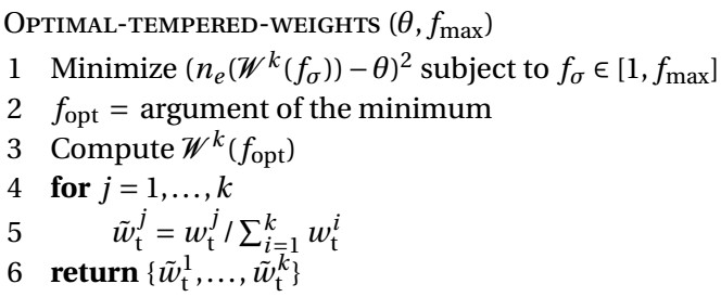
2.1.2. Optimal tempering factor
The tempering factor can be chosen arbitrarily, for example would correspond to taking the average of log-likelihood over N observation points of the mismatch. Instead of fixing a value for f𝜎, we propose a method to adaptively choose optimal f𝜎. It is inspired by the formulation of corrected PoPEx weights.
Let us consider a set of k tempered weights with parameter f𝜎:
| (8) |
| (9) |
Suppose that the target value of the minimal number of effective weights 𝜃 is chosen by the user, who also specifies the value of fmax which will be the max bound for f𝜎. We will define f𝜎 as optimal if it is such that the number of effective weights ne equals at least 𝜃 and f𝜎 ∈ 1,fmax is as small as possible. This can be translated into the following optimization problem:
| (10) |
The tempering framework can be summarized in the form of an algorithm. It takes as input: 𝜃—the target number of effective weights; fmax—the max bound for the tempering factor. The algorithm is as follows:
Once the models are generated (PoPEx stops after a number of steps predefined by the user), PoPEx uses weights for generating predictions. While it is possible to use the tempered likelihood instead of the exact likelihood during PoPEx sampling, we do not use this approach in this study. PoPEx is run with the correct (exact) likelihood for the problem at hand, and the tempered likelihood is only applied for computing predictive weights.
In this study and in previous ones [Jäggli et al. 2017, 2018; Dagasan et al. 2020], PoPEx was coupled with the Direct Sampling (DS) MPS algorithm to generate the categorical fields. More precisely, we use the DeeSse implementation with multi-resolution features [Straubhaar et al. 2020]. The multi-resolution capability (Gaussian pyramids) is a technique allowing for improved reproduction of patterns at different scales.
2.2. ESMDA + DS pyramid
The second inversion method that we will compare is the one proposed by Lam et al. [2020]. It is based on the ensemble smoother with multiple data assimilation (ESMDA) coupled with DS with Gaussian pyramids. ESMDA [Emerick and Reynolds 2013] runs for a predefined number of steps Na (parameter given by the user, also known as number of data assimilations), and at each iteration k ∈{ 1,2,…,Na} the ensemble Ne of models is updated to . We use subscript here for the model index and superscript for the iteration index. The index 1 corresponds to the initial (prior) ensemble, and the ensemble after Na data assimilations will have index Na + 1. We based the algorithmic implementation of the method on the paper by Emerick [2016].
Contrary to PoPEx, in the ESMDA framework, a model is a vector of real values (not discrete) and the described method concerns matching data represented by continuous values. The main novelty of the approach proposed by Lam et al. [2020] is the way of conditioning categorical simulations with continuous variables. Therefore, the ESMDA procedure is a standard one, but the data that is assimilated is used to condition categorical simulations. In this subsection, we will review briefly how it is done. We need two ingredients: a procedure for generating an initial ensemble of models, which is a vector of continuous parameters, and a procedure to generate categorical models based on such a vector.
2.2.1. Coupling DS and ESMDA
The ensemble of models is generated using the following steps.
We use the multi-resolution option of the DeeSse code [Straubhaar et al. 2020] to generate unconditional realizations. The fine-scale realizations are categorical but the DeeSse simulation algorithm starts by generating a pyramid of lower-resolution continuous images over the same grid. The low-resolution continuous images guide the simulation of the higher-resolution categorical images Lam et al. [2020]. The link between the continuous and categorical variables is established on the training image using Gaussian kernels to blur and represent the field at a lower resolution. At the coarse resolution, a fraction f of the total number of cells is sampled to obtain an ensemble of pyramid values (now continuous) at fixed locations , with , where k is the iteration index, i the ensemble member index, and Nm the number of conditioning locations. represents a Gaussian pyramid value at a location with index j. While it would be possible to use directly vectors in the ESMDA procedure, it is not a good idea, because these parameter distributions are not necessarily Gaussian and ESMDA performance will be hindered. Therefore, Lam et al. [2020] suggest using normal score transform, as proposed in the study of Zhou et al. [2011].
The normal score transfer function is constructed for each parameter in the vector and is kept fixed for the entire data assimilation process. Let Fj for all j ∈{ 1,2,…,Nm} be the cumulative distribution function (CDF) deduced from the ensemble . For each pyramid location, j corresponding Fj is computed with its inverse and they are stored. Now the direct normal score transform is defined:
| (11) |
| (12) |
Finally, the vector is obtained from the initial ensemble:
| (13) |
| (14) |
2.3. DREAM-ZS + WGAN
The third inversion method is DREAM-ZS used with a Wasserstein Generative Adversarial Network (WGAN). The approach was initially proposed by Laloy et al. [2018], we use it with only a slight modification: we employ a Wasserstein GAN instead of a Spatial GAN.
2.3.1. DREAM-ZS
DREAM-ZS is a modified Metropolis sampler, sampling multiple chains which exchange information using an archive of past models [Laloy et al. 2018, 2017]. Metropolis samplers generate proposals and accept them if their likelihood is higher, or with a probability if it is lower. In a standard Metropolis sampler, chains would not communicate with each other, which makes it easily parallelizable, but requires removing outlier trajectories; this results in a slower convergence. DREAM-ZS provides a way to allow efficient parallelization and communication between the chains; hence avoiding the necessity of removing outlier chains. Usually, the sampler is run unless a convergence criterion is satisfied [for example Gelman and Rubin 1992] but in practical cases with a large amount of data, the convergence might not be achieved in a reasonable number of iterations [Laloy et al. 2018]. Therefore, we simply run here Nc chains during a predefined number of iterations T and use the two last recorded samples from each chain to form the posterior. Samples are recorded every K iterations. Our implementation uses a Wasserstein GAN (WGAN), instead of a spatial GAN (SGAN) as it was suggested by Laloy et al. [2018], because WGANs are known to be more stable, and easier to train for different training data sets. More details on our WGAN setup are given in the next subsection. The details of our implementation are based on the MT-DREAM-ZS paper Laloy and Vrugt [2012] but we do not use the multiple tries (MT) technique. Our implementation essentially corresponds to MT-DREAM-ZS with one trial. The algorithm for computation of crossover values is based on the work of Vrugt et al. [2009].
The parameter space is the latent space of the GAN, x is the parameter vector of length d: . We will use to denote the archive, which is a collection of past models used to create new proposals in the Markov chain; the archive is updated every K iteration. The posterior should be formed by taking samples from and ignoring initial and burn-in samples. In our setting, we propose to take the last 2Nc samples from , where Nc is the number of chains. It means that the two last archived samples of each chain are conserved for the posterior.
The initial archive is composed of Np (number of prior samples in the archive) random normal vectors:
| (15) |
In each chain i ∈{ 1,2,…,Nc}, for all t < T, (t is the iteration index) a transition from the current point xi to a new point is proposed. There are two ways to generate a proposal point in DREAM-ZS: either by the parallel update or by the snooker update. The snooker update is applied with a certain frequency (fs), otherwise, parallel update is applied. The proposed point is always accepted if its likelihood is higher than L(xi), otherwise it is accepted with probability . If the point is accepted, we set , otherwise, the state of the chain remains unchanged. Every K iterations the archive is updated:
| (16) |
The snooker update was described by ter Braak and Vrugt [2008] and parallel update by Laloy and Vrugt [2012]: Laloy and Vrugt [2012] suggested that every fifth iteration, the jump size 𝛾 is set to 1, in our implementation, it is set every fifth iteration on average.
The final piece of the DREAM-ZS algorithm is the implementation of crossover values, which has two ingredients: determination of CR value for each chain, and the CR distribution improvement. Unlike Vrugt et al. [2009], we improve the CR distribution at every iteration until the end of the DREAM-ZS algorithm.
The determination of CR value for the chain i proceeds as follows. Supposing that we have a probability vector such that pm ∈ [0,1] and . The value vi is drawn from a categorical distribution with possible values {1,2,…,nCR} and corresponding probabilities p. Let us use ℳ({1,2,…,nCR},p) to denote such a categorical distribution. The corresponding CR value is set as: CR = 1∕vi.
Now, we need a way to update the vector p. The initial values of elements for the vector are pm = 1∕nCR for m ∈{ 1,2,…,nCR} and these values are recalculated after each DREAM-ZS iteration. Let v ∈{ 1,2,…,nCR}N c be the vector with the sampled CR values for each chain. Let us define vectors , initialized with zero vectors, whose elements are updated as follows:
| (17) |
| (18) |
2.3.2. WGAN
Generative adversarial neural networks (GAN) can learn a complex mapping between a latent space and the space of two-dimensional images [Goodfellow et al. 2016]. In this work, we decided to use the Wasserstein GAN [Arjovsky et al. 2017] with gradient penalty term, which is claimed to be robust for changing architecture of the network [Gulrajani et al. 2017]. GANs are composed of two neural networks: a critic (discriminator) and a generator. The generator maps the latent space vectors to the image space. The critic is fed by the output from the generator or real images (the images from the training set) and predicts if the images are fake (generated images) or not. The goal of the generator is to deceive the critic so that it cannot distinguish the generated images from the images of the training set. Typically, for an epoch (GAN training iteration), the critic is optimized several times after a single generator training.
In our case, the latent space has d dimensions and the images represent the geology. While the generated images (GAN output) have values between [−1,1], they can be converted to binary images by applying a threshold (0). However, the threshold is not applied when evaluating the likelihood of the model. Instead, the physical parameters are linearly transformed from the pixel values, with − 1 and 1 corresponding to the exact values according to facies. The training set contains all the possible extractions from the TI of the size 128 × 128. The training batch size is 64, the learning rate 1 × 10⁻⁴, the ADAM optimizer was used with beta parameters: 0.5 and 0.999. There are 5 critic iterations per generator iteration, and the lambda term for the gradient penalty was set to 10. The architectures of the generator and the critic are shown in Tables 1 and 2, respectively.
Layers of the convolutional neural network used for generator
| Layer type | Kernel | Stride | Padding | Output shape |
|---|---|---|---|---|
| Input | 50 | |||
| 2D transp. conv. | 4 × 4 | 1 × 1 | 0 × 0 | |
| Batch norm, ReLU | 1024 × 4 × 4 | |||
| 2D transp. conv. | 4 × 4 | 2 × 2 | 1 × 1 | |
| Batch norm, ReLU | 512 × 8 × 8 | |||
| 2D transp. conv. | 4 × 4 | 2 × 2 | 1 × 1 | |
| Batch norm, ReLU | 256 × 16 × 16 | |||
| 2D transp. conv. | 4 × 4 | 2 × 2 | 1 × 1 | |
| Batch norm, ReLU | 128 × 32 × 32 | |||
| 2D transp. conv. | 4 × 4 | 2 × 2 | 1 × 1 | |
| Batch norm, ReLU | 64 × 64 × 64 | |||
| 2D transp. conv. | 4 × 4 | 2 × 2 | 1 × 1 | 1 × 128 × 128 |
| Tanh | 1 × 128 × 128 |
Layers of the convolutional neural network used for critic
| Layer type | Kernel | Stride | Padding | Output shape |
|---|---|---|---|---|
| Input | 1 × 128 × 128 | |||
| 2D conv. | 4 × 4 | 2 × 2 | 1 × 1 | |
| Instance norm, leakyReLU | 64 × 64 × 64 | |||
| 2D conv. | 4 × 4 | 2 × 2 | 1 × 1 | |
| Instance norm, leakyReLU | 128 × 32 × 32 | |||
| 2D conv. | 4 × 4 | 2 × 2 | 1 × 1 | |
| Instance norm, leakyReLU | 256 × 16 × 16 | |||
| 2D conv. | 4 × 4 | 2 × 2 | 1 × 1 | |
| Instance norm, leakyReLU | 512 × 8 × 8 | |||
| 2D conv. | 4 × 4 | 2 × 2 | 1 × 1 | |
| Instance norm, leakyReLU | 1024 × 4 × 4 | |||
| 2D conv. | 4 × 4 | 1 × 1 | 0 × 0 | 1 |
3. Test case
3.1. The inverse problem
We consider a pumping test in a confined aquifer of thickness 10 m. At the beginning of the test, the hydraulic heads are uniform and constant at 0 m. Water is pumped with a constant discharge rate of 0.08 m3∕s during 2 h. The hydraulic heads are recorded in the pumping well and nine piezometers in the vicinity of the pumping well (Figure 1 and Table 3). The hydraulic heads are recorded every 100 s, so that 72 measurements are available at each of the 10 locations, which makes up for a total of N = 720 measurement points (Figure 2).
Position of the pumping well (W) and nine piezometers (A–I) in the pumping test.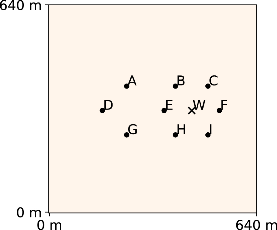
Time series of hydraulic heads recorded at nine piezometers (A–I) and the pumping well (W).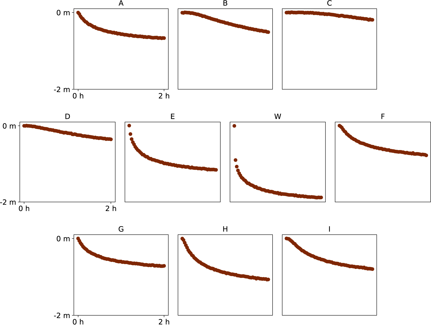
Positions of piezometers (x, y coordinates), corresponding columns and row indexes, and labels
| x (m) | y (m) | Column index | Row index | Label |
|---|---|---|---|---|
| 242.5 | 392.5 | 48 | 78 | A |
| 392.5 | 392.5 | 78 | 78 | B |
| 492.5 | 392.5 | 98 | 78 | C |
| 167.5 | 317.5 | 33 | 63 | D |
| 357.5 | 317.5 | 71 | 63 | E |
| 442.5 | 317.5 | 88 | 63 | W |
| 527.5 | 317.5 | 105 | 63 | F |
| 242.5 | 242.5 | 48 | 48 | G |
| 392.5 | 242.5 | 78 | 48 | H |
| 492.5 | 242.5 | 98 | 48 | I |
3.2. The reference set-up
The data presented in the previous section were obtained from a synthetic setup. We will refer to it as the reference. It is not the solution to the inverse problem framed in a probabilistic manner. It is rather a model which has a very high likelihood, given the data. The domain has an extension of 640 m by 640 m. The petrophysical parameters are modeled using a categorical 2D field with two geological facies: a permeable (channels or ellipsoidal deposits, labeled with 1) and a less permeable matrix (labeled with 0). The area is discretized using a regular grid with cells of size 5 m by 5 m, thus the grid contains 128 by 128 cells. The two geological facies have constant hydrogeological parameters (Table 4). The boundary conditions are constant head values at all edges, equal to 0 m, and at the beginning of the pumping test, hydraulic charge equals to 0 m everywhere in the domain. The reference field was created using the DeeSse software, which is an implementation of Direct Sampling algorithm with pyramids [Straubhaar et al. 2020]. An extended image of a channelized aquifer was used as the training image (Figure 3). We chose to run the DeeSse in the Direct Sampling Best Candidate (DSBC) mode, which boils down to choosing a threshold of 0 in the standard Direct Sampling, or very small, close to 0, if the software does not allow for non-positive input. The maximal scan fraction was set to 0.01 and the number of neighboring nodes to 40. Two pyramid levels were used, with the reduction by 2 in each direction at every level. The groundwater flow was simulated using the FloPy python package [Bakker et al. 2016], which is a wrapper for the MODFLOW software [Hughes et al. 2017]. To emulate the measurement error, the obtained values of hydraulic heads were corrupted with Gaussian noise with mean 0 m and standard deviation 0.005 m. These data will be used as input for the different inversion procedures.
Hydrogeological parameters of different geological facies considered in the study
| Less permeable (0) | More permeable (1) | |
|---|---|---|
| Hydraulic conductivity (m/s) | 1 × 10⁻⁴ | 1 × 10⁻² |
| Specific storage (m−1) | 5 × 10⁻⁴ | 5 × 10⁻⁵ |
| Porosity | 0.4 | 0.3 |
Reference (true) training image, used to generate the reference (“true”) field. Data from Zahner et al. [2016].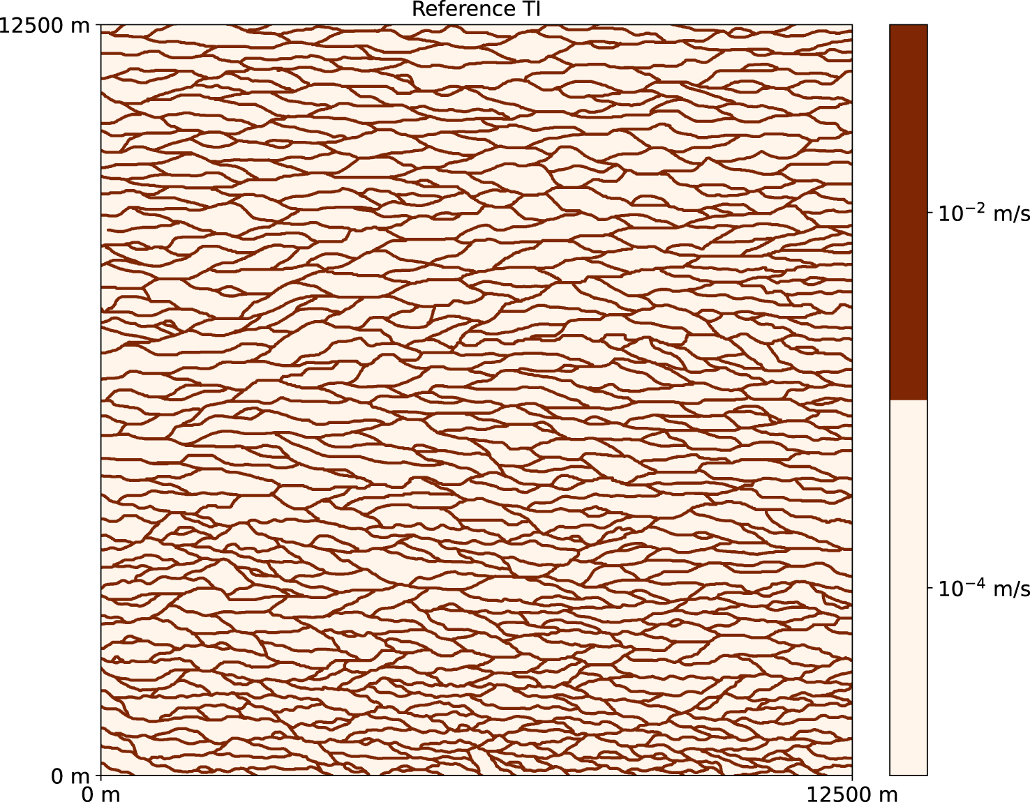
To evaluate the quality of the inversion methods, we use in addition a prediction problem. The prediction data will not be used by the inversion algorithms. Here we consider, the prediction of the 10-day groundwater protection zone, it is also referred to as the 10-day capture zone [van Leeuwen et al. 1998]. It is calculated in a slightly different setup but with the same geological model and its properties. The boundary conditions are prescribed heads equal to 1 m on the left boundary, 0 m on the right boundary and interpolated between those two values on the upper and the lower boundaries. A constant pumping rate of 0.04 m3∕s is imposed at the well and forward particle tracing is performed on the steady-state solution of groundwater flow. The 10-day zone contains each location (pixel), from where groundwater reaches the pumping well in less than 10 days.
The reference field (A) used as the synthetic reality (considered unknown) and the corresponding 10-day groundwater protection zone (B).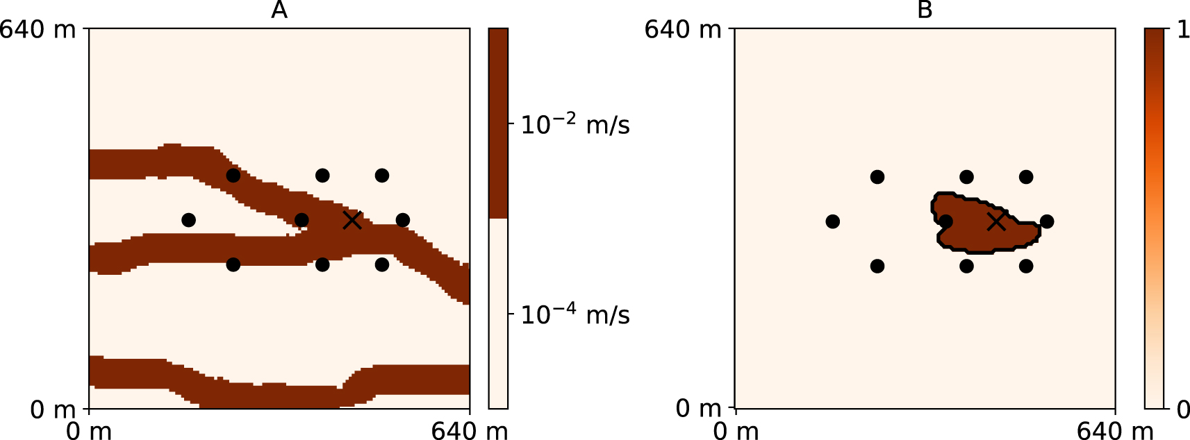
3.3. Inversion set-up
We will perform the inversion three times for each method. Every time, we use a different training image. The baseline case uses the reference TI, the two other cases use a different one. In this way, the robustness of the inversion methods can be tested. The two other training images were generated with the TI generator tool [Maharaja 2008] in the AR2GEMS software. Their size is identical to the one of the original TI. The first is a channelized medium with disjoint channels, and the second represents ellipsoidal deposits. TIs have the same proportion of facies as the original TI. We will refer to them as “Channels TI” (Figure 5) and “Ellipses TI” (Figure 6).
“Channels TI”, an alternative training image.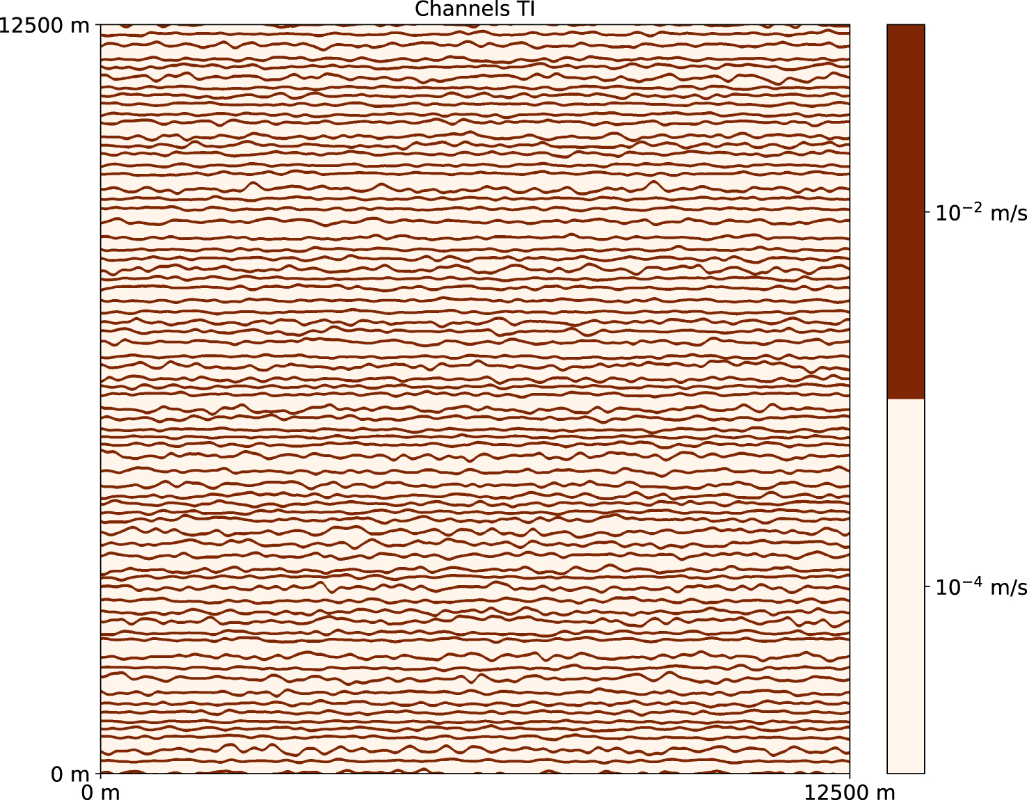
“Ellipses TI”, an alternative training image.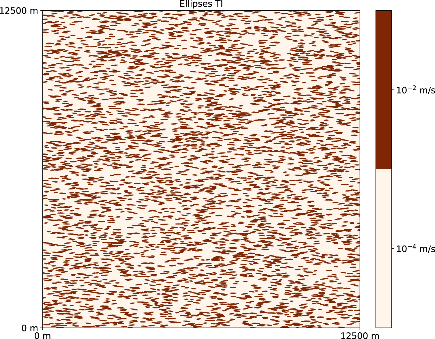
Both PoPEx and ESMDA benefit from the same geostatistical engine as the original reference; it means that the same DeeSse parameters are used in PoPEx + MPS and in ESMDA + MPS to generate the reference. In theory, it is possible (but highly unlikely) that PoPEx samples the same model as the reference. It might not be the case for ESMDA, as it imposes dense conditioning on a coarse grid, but very similar models can be produced. The fact that PoPEx and ESMDA use DeeSse, gives them an edge compared to DREAM-ZS+GAN, as the reference is a realization generated by DeeSse (therefore not present in the TI). GAN is trained on images cut from the TI and learns to develop similar realizations, but it does not have access to samples simulated with MPS.
It is important to note that the three inverse methods identify a different number of unknowns. For PoPEx, the number of unknowns is simply the number of grid cells in the domain, i.e. (128 × 128) = 16,384. For ESMDA, the number of unknowns is reduced, as compared to PoPEx, because they are the continuous values on the low-resolution map used to constrain the MPS realizations. In the example, two pyramid levels are added, each one being obtained by dividing by 2 the number of cells along each axis, and 20% of the cells in the coarse level are updated by the procedure, which results in a total of 0.2 × (128 × 128)∕(4 × 4) ≈ 204 unknowns. Finally, for DREAM-ZS+GAN, the number of unknowns is the size of the latent Gaussian vector used as input to the GAN (Table 1), and it is only 50. However, note that the above calculation omits the fact that, for the two first approaches, the values in the grid cells are correlated via the MPS statistics, and it is therefore difficult to estimate the actual dimension of the underlying parameter space.
PoPEx was run with the following parameters: 32 parallel processes, and for a total of 50,000 iterations (50,000 forward runs), the maximal number of conditioning points is 10. The choice of the number of parallel processes depends on available computing resources, in our case it was adjusted to the number of cores in a computing node. The number of forward runs and conditioning points are similar to values suggested in the paper introducing the parallel PoPEx algorithm [Jäggli et al. 2018], where the problem size was of comparable dimensions. ESMDA was run for 16 iterations (16 data assimilations), the size of ensemble is 128 (a total of 2048 forward runs) and number of parallel processes 32. The chosen parameters are again close to those used in the paper which introduced the method Lam [2019], which also suggested that using larger number of iterations would not lead to better results. DREAM-ZS was run for total T = 5000 iterations with 32 parallel chains (160,000 forward runs). The initial archive size is set to 500. The size of the latent vector is d = 50. Frequency of snooker update is 0.1, 𝛿max = 1, and nCR = 3, according to recommendations for standard parameters. To study the convergence, we set a fairly low value for K, equal to 10, but the value 100 should be sufficient for the chosen number of iterations. Moreover, we set b = 0.05 and b⋆ = 1 × 10⁻⁶. These parameters have been tested in the paper presenting the DREAM-ZS with GAN for a hydrogeological problem [Laloy et al. 2018]. For practical reasons, to avoid too long computing times, we chose a smaller size of the latent vector and set a limit on the number of iterations.
4. Comparing the results
Since our numerical experiments involve a large number of results, we need to use summary statistics to compare the different methods efficiently. For that purpose, we will use three metrics for comparing the quality of the results:
- The first metric indicates how well the measurements are reproduced by the simulation ensemble. Each continuous measured value will be compared with the ensemble of simulated values. A score that allows for such a comparison is the continuous ranked probability score (CRPS) used to assess probabilistic forecasts [Gneiting et al. 2007; Gneiting and Raftery 2007].
- The second metric indicates how well the protection zone is predicted. In this case, a discrete (categorical) value is compared with a probability for each point using a quadratic score [Gneiting et al. 2007].
- Finally, the third metric indicates how well the geology is identified. For that purpose, we use the average of pixel-by-pixel quadratic scores of predicted facies.
Below, we recall the definition of the CRPS and quadratic (Brier) scores.
4.1. CRPS score
The continuous ranked probability score (CRPS) is given by:
| (19) |
In our context, the crps score will be averaged for all measurement points:
| (20) |
4.2. Quadratic (Brier) score
The quadratic score was first introduced by Brier [1950] to quantify forecasts of categorical variables expressed in terms of probabilities. The quadratic (aka Brier) scoring rule is given by:
| (21) |
In our context, we will average the Brier score over all locations where it is predicted if that location is in the groundwater protection zone. Let pk be a probabilistic forecast if point k is in groundwater protection zone, and lk true category (in this case binary) of point k. The average Brier score is then given by:
| (22) |
5. Results
For each of the methods and for each of the TIs, we report prior data coverage and posterior data match, and corresponding prior and posterior probability maps (groundwater protection zone, facies) with examples of realizations. We also compare the convergence of the methods with respect to the number of forward calls.
5.1. Prior distributions
The prior groundwater protection zones are essentially circular (Figure 7), as the most probable event is that the well is placed in the less impermeable facies. Such a configuration results in a large (and unrealistic) drawdown. If we look more closely at the prior groundwater protection zone maps, we can see a second mode, which is an ellipse. This occurs when the pumping well intersects a channel. Such a zone shape is visible for the Channels TIs (Figure 7).
Prior probability distributions obtained with the Channels TI for the groundwater protection zone (left column), and the channel occurrence (middle column). The black contours correspond to the reference. The right column shows one example of realization. The top row shows results obtained with PoPEx, the middle row shows results obtained with ESMDA, and the bottom row shows results obtained with DREAM-ZS. The colormap is the same as for Figure 4B.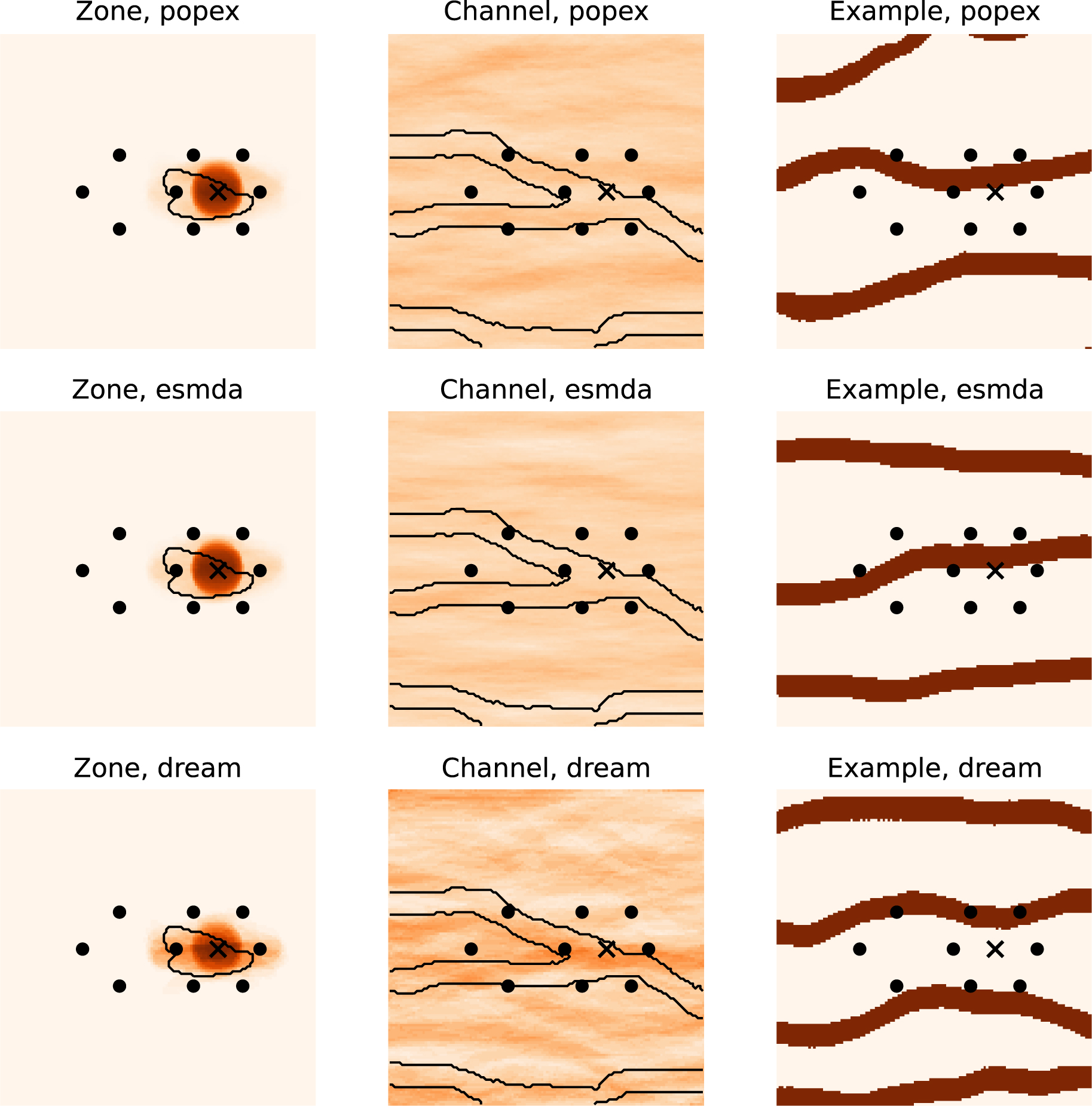
The channel prior probability maps are roughly homogeneous for all the simulation methods and training images (for example, see Figure 7). This is expected as we did not impose any prior conditioning data, the prior probability of a channel corresponds then to the proportion of channels in the training image.
For the drawdown curves in the piezometers and pumping well, the prior distribution shows wide confidence intervals, as can be seen for DREAM-ZS and Ellipses TI for example (Figure 10). The true data are usually within the 95% confidence intervals, but there are some exceptions, and it happens that some head data lie outside of this range.
5.2. Posterior distributions
The confidence intervals for the drawdown curves are very much reduced, and they mostly match the data well (Figures 8–10).
Prior and posterior distributions of the drawdown curves obtained with PoPEx and the Ellipses TI at the nine piezometers (A–I) and pumping well (W). The observed data is marked with thick brown dots, the median of the posterior distribution with thin black line, the 95% confidence intervals of the posterior are shown as dark shaded region, and those of the prior distribution are shown as the light shaded region.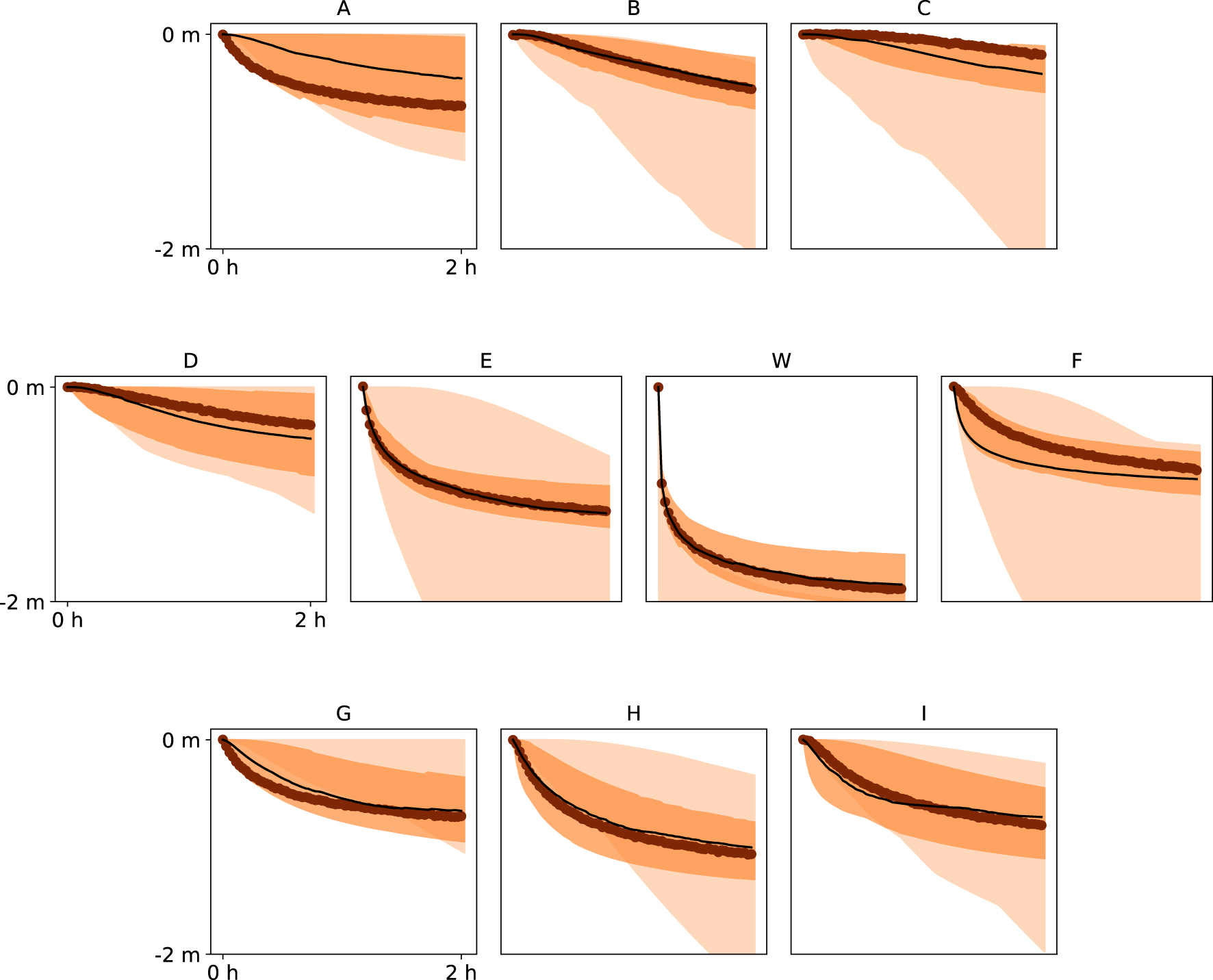
Prior and posterior distributions of the drawdown curves obtained with ESMDA and the Ellipses TI at the nine piezometers (A–I) and pumping well (W). The observed data is marked with thick brown dots, the median of the posterior distribution with thin black line, the 95% confidence intervals of the posterior are shown as dark shaded region, and those of the prior distribution are shown as the light shaded region.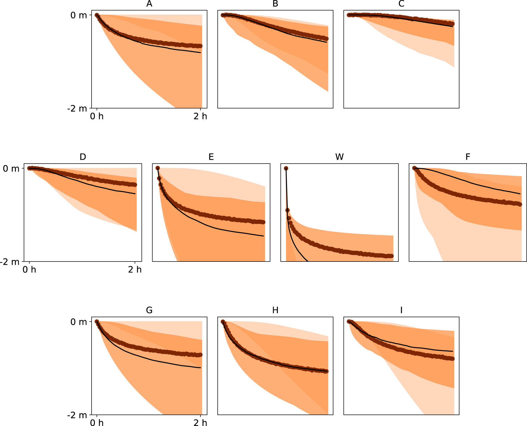
Prior and posterior distributions of the drawdown curves obtained with DREAM-ZS and the Ellipses TI at the nine piezometers (A–I) and pumping well (W). The observed data is marked with thick brown dots, the median of the posterior distribution with thin black line, the 95% confidence intervals of the posterior are shown as dark shaded region, and those of the prior distribution are shown as the light shaded region.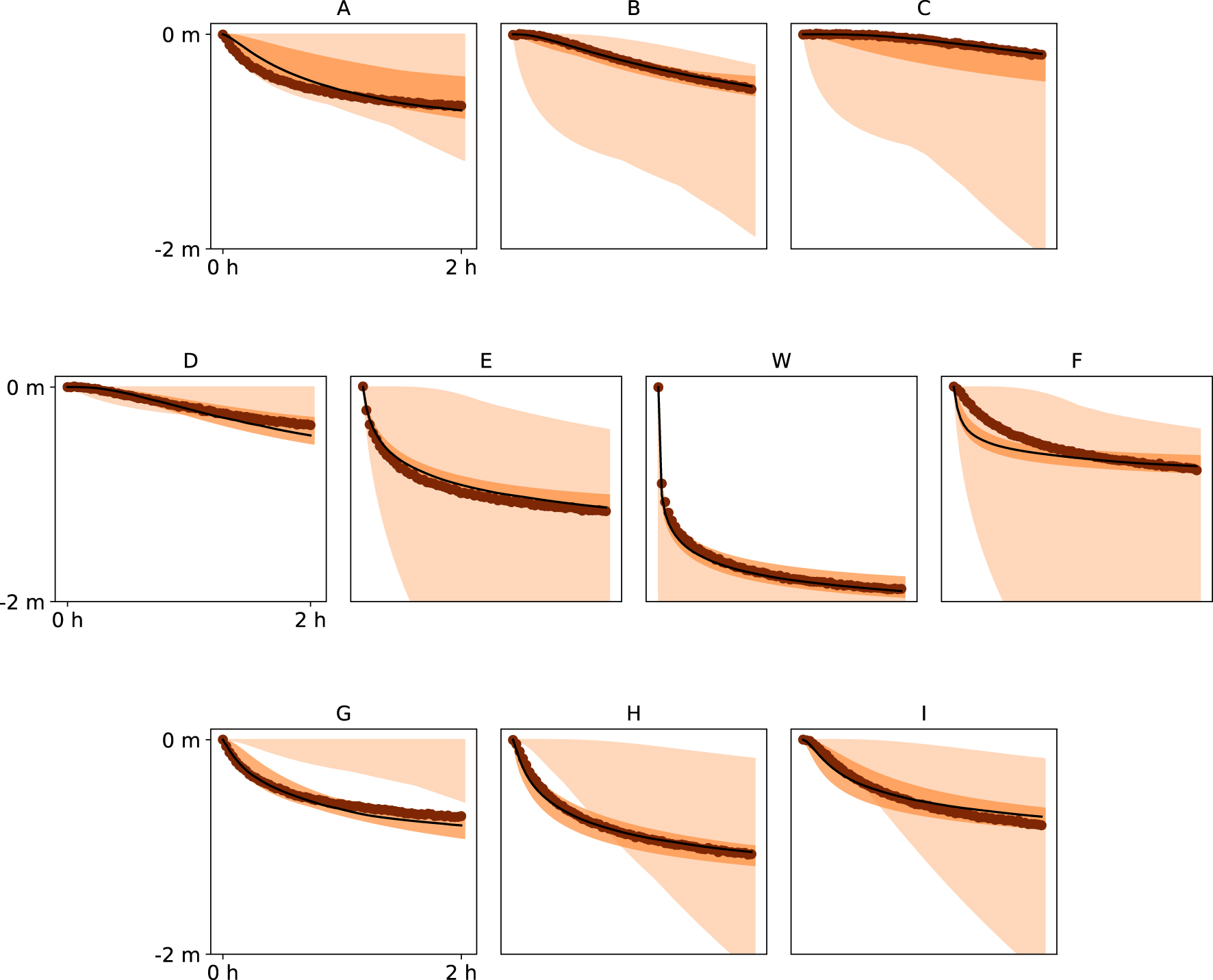
Even if we do not show the figures here for the sake of brevity, the posterior distribution computed using the reference TI with all the methods achieved a satisfactory data fit, with DREAM-ZS and PoPEx producing very narrow confidence intervals and an excellent match and ESDMA producing wider confidence intervals.
With the Channels TI, PoPEx produced wider confidence intervals, and some piezometric data (A, F, H, I) are not matched perfectly, but the fit is reasonable. ESMDA achieved slightly worse piezometer data fit, but the well data is reproduced poorly, giving a high probability of the well placement in (or close to) the less permeable region. DREAM-ZS achieves a very close fit and provides narrow confidence intervals.
The Ellipses TI is the most difficult one. PoPEx does not match the data well for some piezometers (A,C,F) and produces quite wide confidence intervals (Figure 8). ESMDA produces wide confidence intervals, and the head data in the pumping well are poorly represented (Figure 9). DREAM-ZS produced very narrow confidence intervals, but the data are sometimes not very well matched (Figure 10F).
In terms of posterior probability maps, all methods solved reasonably well the inverse problem in the reference case. The protection zone probability maps are very close to the reference protection zone for all methods (Figure 11). The permeable facies probability maps were able to represent the bifurcation. We note however some general trends to predict with over-confidence certain geological features. For PoPEx, on the right side of the map, the channel goes straight with a high probability, while in the reference it goes slightly to the bottom. For the ESMDA algorithm, the posterior probability map suggests some “eye” feature to the left of the bifurcation. This pattern is not suggested by PoPEx. For DREAM-ZS, the “eye” structure is even more pronounced and the same map indicates with high probability a channel at the bottom, which only partially coincides with the channel in the reference realization. These rather high posterior probabilities of the presence of certain geological features that are not present in the reference seem to correspond to some artifacts of the methods and not to features suggested by the statistics of the TI.
Posterior probability maps obtained with the true TI for the groundwater protection zone (left column), and the channel occurrence (middle column). The black contours correspond to the reference. The right column shows one example realization. The colormap is the same as for Figure 4B.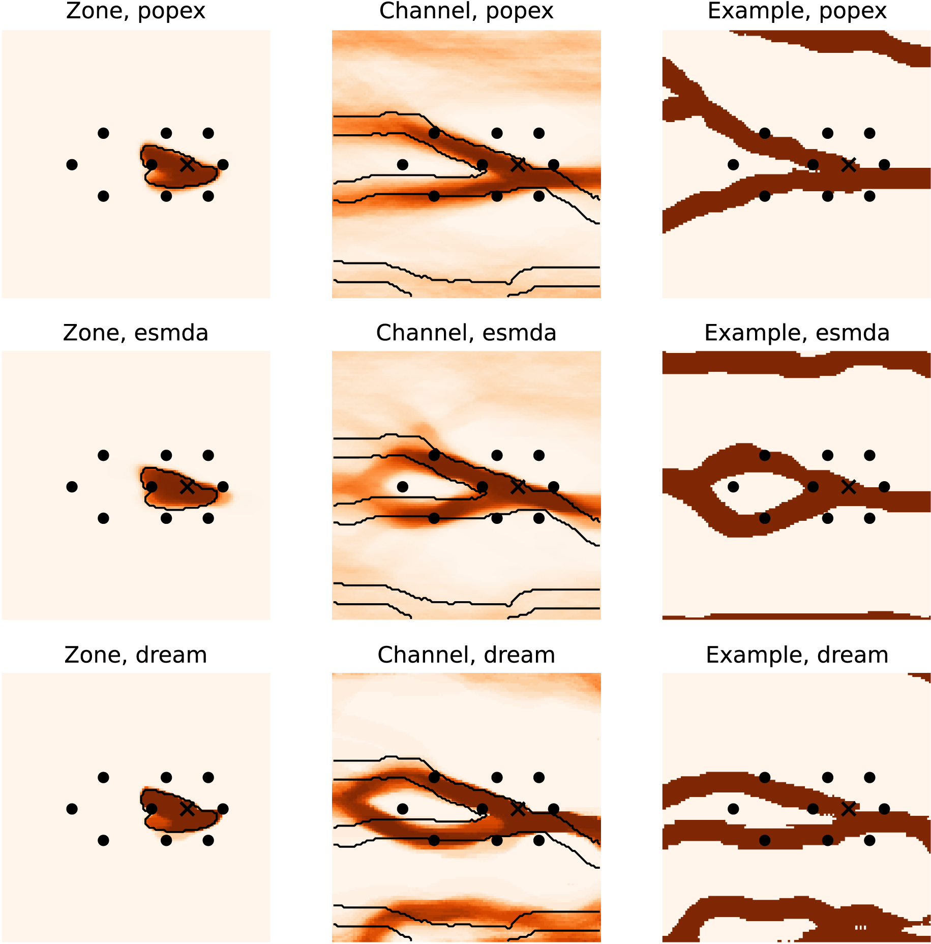
The case of the Channels TI (Figure 12) posed more challenges for the inversion algorithms. The protection zone was only very well represented by the DREAM-ZS method. The zone obtained with PoPEx is more elongated and less influenced by the bifurcation. Indeed, PoPEx indicates a higher probability of channel only in the lower branch. Due to this TI with disjoint channels, it had difficulties in reproducing the branching of channels. ESMDA did not attribute a high probability of permeable facies near the pumping well. However, it managed to find the double channel on the left side of the field. DREAM-ZS performed best in reproducing the bifurcation, but it also displays channel artifacts in the upper part of the image.
Posterior probability maps obtained and example realizations with the Channels TI.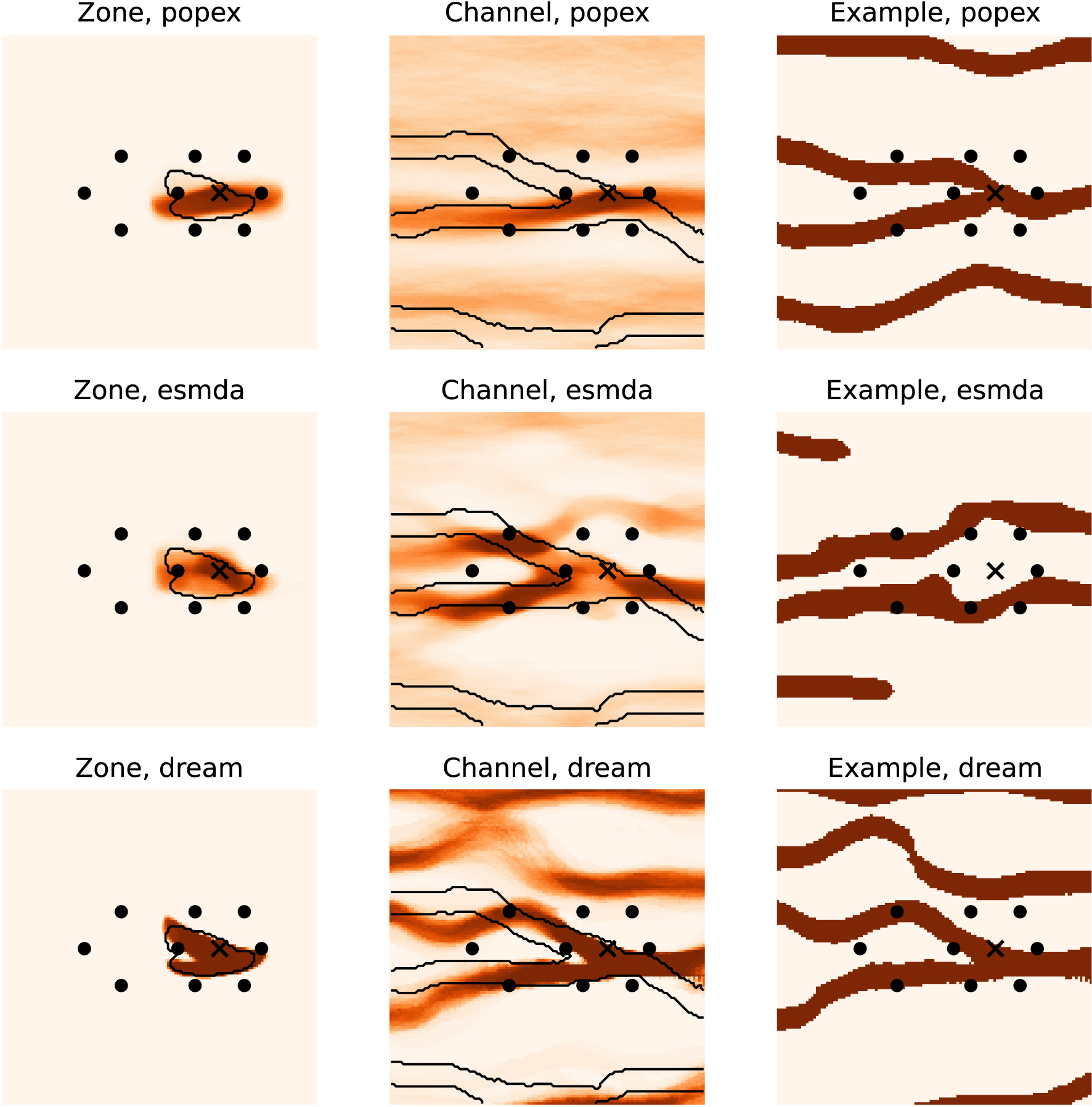
The Ellipses TI can be considered as the hardest case, due to the disconnected nature of the high permeability features (the ellipses). The solution provided by PoPEx can be thought of as the most conservative, as it only places a blurred region of higher channel probabilities around the pumping well (Figure 13). The advantage of this solution is the absence of a high probability of channels in spurious zones. Nevertheless, the protection zone is not accurately reproduced. ESMDA placed a smaller protection zone than it should be and indicated with high certainty the presence of channels in regions where they should not be. DREAM-ZS provides the most contrasted probability maps and places incorrect geological features in the whole area.
Posterior probability maps and example realizations obtained with the Ellipses TI.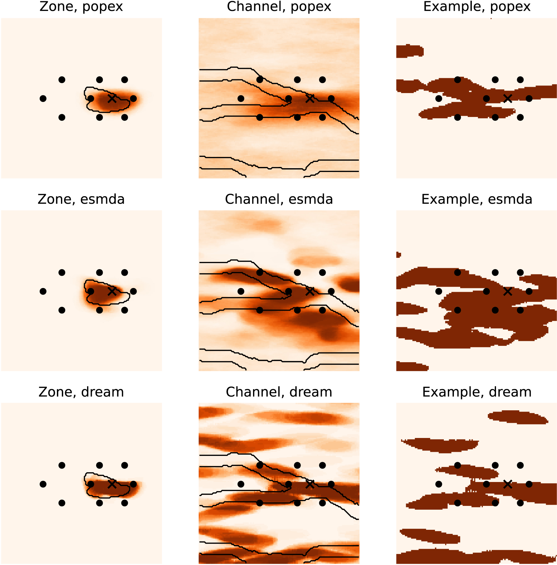
5.3. Convergence and quality metrics
The previous comparison of the posterior distributions shows that it is not simple to compare visually the results. Therefore, in this section, we compare the convergence of three quality metrics to get a better understanding of the performances of the methods. We grouped the convergence plots by methods in Figure 14. The quality metrics are plotted as a function of the number of forward model runs since these runs constitute the most expensive computational cost during the inversion.
Convergence of the posterior predictions, as measured by different scores (columns) for every method (rows). Each plot compares the curves for different TIs.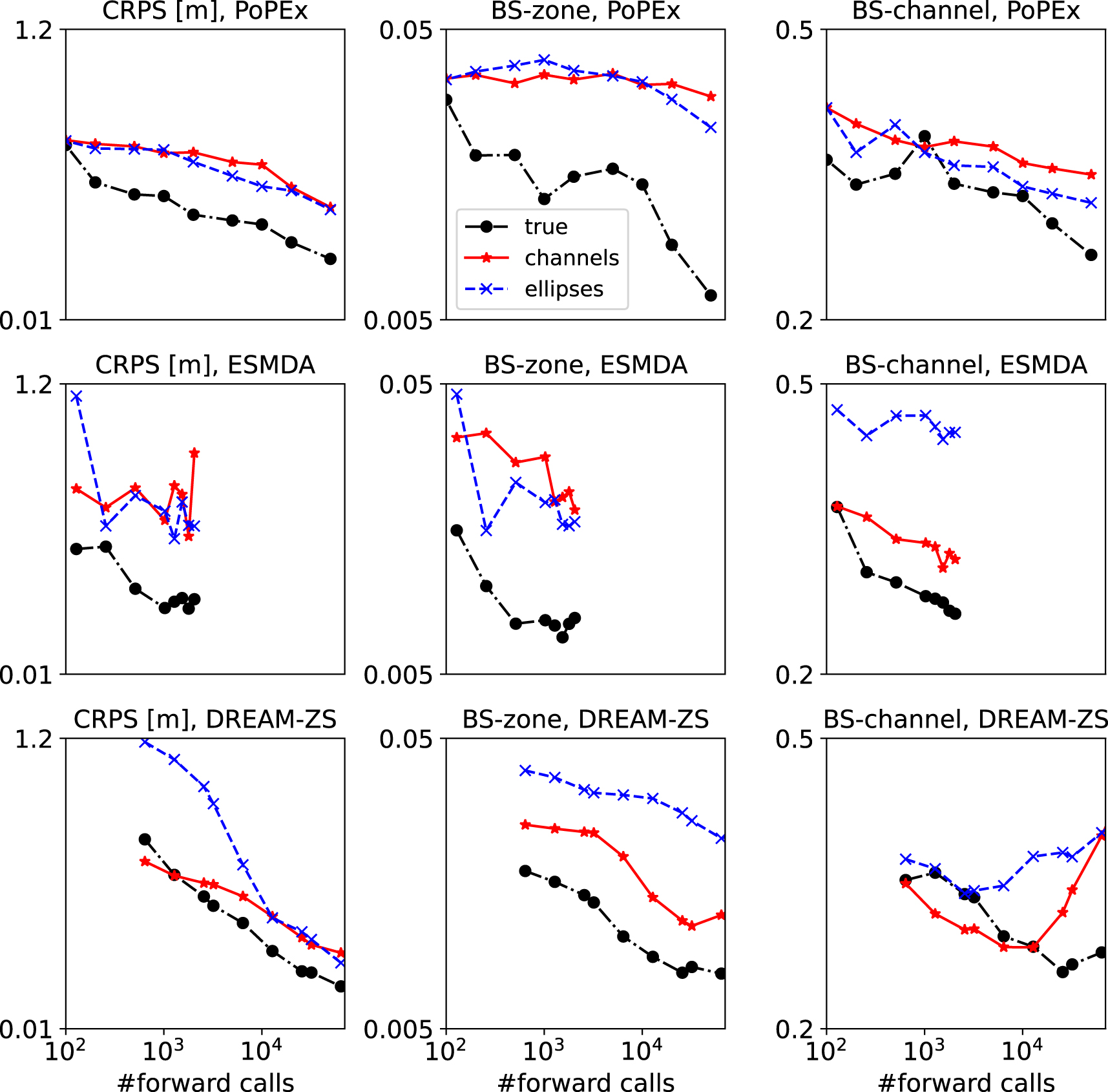
Figure 14 shows that all the methods produced the best results (smaller values of the quality indicators) for the true training image. The methods also converge, i.e. the errors diminish, with the number of forward calls (iterations) for the true training image. Generally, the scores are similar or better for the channel TI than for the Ellipses TI. While different scores show similar trends for the same case, a good CRPS score does not necessarily imply a good Brier score. The most notable example of the lack of correlation is the case of the DREAM-ZS algorithm. The CRPS score goes down for all TIs rather fast, and the scores for Channels TI and Ellipses TI are close. However, when comparing the BS-zone scores, the Ellipses TI results become significantly worse than those with the Channels TI. Moreover, the BS-channel score increases after 1 × 10⁴ forward calls. It seems that the realizations collapse on a very similar (and not fully correct) model realization, and produce geological artifacts which are highlighted by this score, while the CRPS score on data match remains low.
When comparing the different methods for the same TIs, we note that ESMDA exhibits a very fast convergence at the beginning and then reaches a plateau. The method stops after relatively few forward runs (as compared to the other methods), and this is related to the choice of the parameter governing the number of data assimilations. Here, the default value of 16 is used [Lam et al. 2020] and is based on recommendations of Emerick and Reynolds [2013]. In a sense, it is the least computationally expensive method, but the achievable quality is limited. Other methods can provide results of better quality, but they need more iterations. DREAM-ZS shows the best convergence for the data match and protection zone reproduction for the Channels TI, but the error diverges for BS-channel and becomes larger than those of PoPEx and ESMDA for the largest number of iterations. We note a slow but steady convergence of PoPEx when using the Ellipses TI, as opposed to ESMDA, which stagnates after the first iterations, and DREAM-ZS, which matches the piezometric data very well but has slow convergence on the BS-zone and even diverges on the estimation of the geological features (BS-channel).
In summary, PoPEX is the method that seems to be the most robust. It converges steadily with the number of forward model calls, and rather fast when the proper training image is given but slowly if a wrong training image is provided. On the contrary, ESMDA always improves the solution very fast for the first iterations even with a wrong training image, but it stagnates rapidly after a few iterations. DREAM-ZS has an intermediate behavior, it can be faster than PoPEx and continues to improve the results when ESMDA stagnates even with a wrong TI. But there are cases where the DREAM-ZS method diverges and the error increases with additional iterations.
6. Conclusions
In this study, we compared three recent stochastic inversion methods capable of inverting categorical fields: Posterior Population Expansion (PoPEx) with multiple-point statistics (MPS), Ensemble Smoother Multiple Data Assimilation (ESMDA) with MPS pyramids, and DREAM-ZS with Wasserstein Generative Adversarial Network (WGAN). A synthetic test case with hydrogeological data (time series of hydraulic heads) was used, and two geological facies were considered. The results were analyzed both for the inversion and for a prediction of the 10-day groundwater protection zone. The quality indicators took into account the reference solution (ground truth represented by the reference solutions) with probability forecasts.
Our main finding is that when the methods were given the correct prior information (represented by a training image), they all achieved reasonable convergence. Even with the wrong priors, some acceptable solutions were obtained. However, the choice of the prior is essential. The convergence was negatively affected when the TI with lenticular deposits was used. The TI with disjoint channels (as opposed to the original TI with bifurcating channels) provided slightly better results than ellipsoidal deposits, but the two wrong TIs deteriorated the results and introduced artifacts. As previously discussed in the inter-comparison exercise of Zimmerman et al. [1998], we also observed that none of the methods performed systematically better than the others for all the criteria that we studied.
The advantage of PoPEx is that it presented the most steady convergence compared with ESMDA and DREAM-ZS, whose scores fluctuated (ESMDA) or even increased (DREAM-ZS) with the number of iterations. PoPEx can also be thought of as the most “conservative”, as it does not introduce “artifacts”, e.g. geological features which are unlikely (outside the informed zone). However, this “conservative” approach leads to poorer data fit and worse predictions of the protection zone in certain cases. In the case of a wrong prior, it rarely performed better than the other methods.
The advantage of ESMDA is its fast convergence. It was able to reasonably identify the permeable zones between the piezometers even with wrong priors, producing patterns not present in the TI, which was needed to match the data. But it also indicated with high certainty some permeability patterns outside this zone that were incorrect. A surprising point, and drawback of the method, is that it did not always place the well in the permeable zone when a wrong prior was used. It resulted in overestimated confidence interval for the well data.
DREAM-ZS often matched the data the best and provided very good protection zone estimates. It was able to generate realizations that had bifurcation patterns without seeing them in the training set. Outside the informed zone, it was often overconfident in placing geological patterns, even to a greater extent than ESMDA. However, the good performance of DREAM-ZS is remarkable, as the reference data was generated using the MPS tool employed by PoPEx and ESMDA. Identifying these geometries should be easier for these methods than for DREAM-ZS. For a fairer comparison, an additional reference realization generated with GAN could be added, but it would require repeating the whole study.
Note that, this study might be extended by including other methods coupling ESMDA with GAN [Bao et al. 2020; Canchumuni et al. 2021], which would be interesting to compare especially with ESMDA + MPS and DREAM-ZS + GAN. Another point is that the results are compared to a single reference field, and not to a probabilistic reference solution, as for example done by Jäggli et al. [2017]. However, such a probabilistic reference solution requires a very large ensemble of unconditional realizations and depends on the simulation technique and the prior. Since we are modifying the prior in our tests, it would be necessary to consider several probabilistic reference solutions to make the comparisons, implying an even higher computational cost.
More generally, the application of these methods to real case studies still needs to be explored before we could give recommendations to the practitioners. First, one needs to extend the methods to the multi-categorical case. PoPEx is capable of handling it, adapting GAN should be straightforward, but ESMDA + MPS must be adapted to account for multiple Gaussian pyramids. In a practical application, identifying the prior or priors requires geological exploration and testing the different priors using for example K-fold cross-validation strategies as shown in Juda et al. [2020]. This is feasible in theory, but may not always be possible because of limited time. Another important unknown is how these different methods would behave when adding borehole data. Making such a comparison was not possible, because the WGAN that we used is not able to generate geological simulations conditioned by borehole data. Finding ways to condition efficiently the GAN is still a research topic. We also did not evaluate how the different methods perform when the quantity of information varies. All these questions show that research on categorical inverse problems is still very open.
To conclude, the approaches presented and compared in this paper include a statistical and spatial model of a categorical field and a stochastic technique for generating or identifying a set of realizations that could match the head data. This is directly inspired by the philosophy that Ghislain de Marsily taught us (see companion paper by White and Lavenue [2022]). We are still pursuing this track with passion, but the road is bumpy and the destination is far from sight.
Conflicts of interest
The authors declare no competing financial interest.
Acknowledgments
The authors thank Augustin Gouy for the preliminary study that he conducted and for sharing his synthetic inversion set-up, which inspired the test case presented in this article.