


 CC-BY 4.0
1. Introduction
As soon as anyone is tempted to find the causes of some observations, an inverse problem emerges. We face inverse problems daily and most of the time, without being fully aware of this. A quite general definition of an inverse problem is finding the causes of observations, while the direct (or the forward) problem would be to assess the effects of some causes. One of the most popular successes in inverse problems is probably the discovery of Neptune by Le Verrier [1846]. His manuscript started with “Je me propose … d’étudier la nature des irrégularités du movement d’Uranus; et de remonter à leurs causes” (I propose ... to study the nature of the irregularities of the movement of Uranus, and to retrieve their causes). Based on observations of unexplained trajectories of Uranus, Le Verrier applied two inverse methods: (i) a parameter estimation trying to find the best parameter set for the mathematical model calculating the interactions between Uranus, Saturn, Jupiter, and the Sun; (ii) a change in the model by adding a new planet (Neptune) and finding its position and mass. He also questioned the uncertainty of existing data and their potential impact on his conclusions. In his quest to explain why Uranus had irregular unexplained trajectories, he expressed the two basic issues arising when formulating an inverse problem: to find parameters for a given model (parameter estimation), and to find both the model and its parameters (model identification).
Most inverse problems are considered as ill-posed in that they contradict, to some extent, the principles of a well-posed problem in the sense of Hadamard [1902]:
- for all admissible data, a solution exists;
- for all admissible data, the solution is unique;
- the solution depends continuously on data.
It can be noticed that these criteria lack mathematical rigor. What is “admissible”? What kind of continuity is required? Even worse, in Geosciences, a unique and stable solution does not need to be a good representation of reality. This might be one of the reasons why inverse methods have been mostly initiated by intuitive reasoning rather than grounded in mathematically sound deductions. In fact, an ill-posed problem should lead to its reformulation. However, some problems can be considered as “morally ill-posed” [Jaynes 1984] due to practical difficulties such as determining the subsurface structure from surface seismic data, or because of small sensitivities such as determining the transmissivity variability from piezometric heads in groundwater modeling, or because of the complexity (chaotic character, i.e., instability) of interactions between individuals or groups such as the mechanics of billiard balls. Many ill-posed problems are thoroughly described in Bertrand [1889]. In hydrogeology, we know that a solution usually exists, but whether it depends continuously on data or is unique has been the topic of many research activities over the last seventy years. The outcome was that the well-posed character of a problem greatly depends on how the problem is formulated.
The first attempt of parameter identification through an inverse method in hydrogeology can be attributed to Bennett and Meyzer [1952] who used a flow net approach to estimate transmissivity. Stallman [1956] developed the first numerical model for parameter estimation by relying upon this flow net approach. This type of approach continued during the 1960s, until Emsellem and de Marsily [1971] showed that the method led to non-unique (arbitrary, as we will see) and unstable solutions. They realized that a well-posed problem was needed for regularization, and that extra information was required to render the solution realistic. These issues were formalized in the GdM’s “thèse d’Etat” [1978], which led to formulating the inverse problem as an optimization procedure minimizing an objective function that penalizes discrepancies between observations and model outputs. However, regularization was still needed.
The goal of regularization is to improve the conditioning of the inverse problem. Numerous approaches can be adopted. But, to add realism beyond conditioning, they should integrate prior information (i.e., a knowledge about model parameters stemming from sources other than head data). The incorporation of prior information was initially introduced by restricting the size of the domain in the parameter space where the solution was supposed to be (i.e., constraints on the parameter values). However, this led to parameters fluctuating spatially between their bounds, which inclined Neuman [1973] to propose an additional “plausibility criterion”. Tihonov [1963a, b] had shown that by simply adding the quadratic norm of the parameters to the objective function, linear regression could become well-posed. Even though this added criterion did not include prior information, it opened the way of using metrics accounting for priors. Note that strict Tikhonov regularization simply promotes smoothness. Carrera and Neuman [1986b] argue that this limitation is fictitious because Tikhonov’s regularization can be used with any appropriate formulation i.e., Tikhonov’s results are valid if the regularization term penalizes any norm of the parameter departures with respect to the prior information. See Engl et al. [1996] for a general overview of Tikhonov regularization.
Part of the instability problem results from trying to estimate too many parameters from a limited amount of data. Therefore, another line of research has been trying to represent permeability fields with a limited number of unknown parameters. This is called parameterization, which can also be seen as a particular regularization method, in the sense that it improves the conditioning of the inverse problem by reducing the number of degrees of freedom (i.e., the number of parameters to estimate). In fact, an adequate parameterization allows for incorporating prior information, both in terms of parameter values and their statistical and spatial distributions. Parameterization can compile “hard” information such as measured parameter values and subjective knowledge (“soft” information) coming from the investigations of different disciplines including geology, geophysics, and hydrology. This “soft” information may also be the result of field works (geologic maps, drilling logs, pumping tests, geophysical surveys) that may provide a reasonably good insight into the acceptable range of parameters and their spatial distribution. Again, words like “reasonably” and “acceptable” cover subjective notions which allow for a lot of creativity. As we will see, this may have been the most lasting contribution of GdM.
The aim of this paper is not to review parameter estimation by inverse methods. Numerous excellent reviews targeting the inverse problem in hydrogeology can be found in Yeh [1986], Carrera [1988], Ginn and Cushman [1990], de Marsilyet al. [2000], Carrera et al. [2005], McLaughlin and Townley [1996], Kitanidis [2007], Oliver and Chen [2010], Zhou et al. [2014], Yeh [2015]. Instead, our goal is to highlight the contributions of GdM in solving the above-mentioned problems (proper formulation, regularization, and parameterization), which are keys for model calibration and predictive uncertainty [Cui et al. 2021].
The paper is organized along two lines. First, we outline the evolution of the formulation of the problem. Second, we review the four main parameterization strategies: zonation, interpolation such as pilot points, embedding geophysical information, and lithological information from modeling. For each strategy, we start from GdM’s work and provide a short review of how his ideas percolated until today. For simplicity (for the readers and the authors), we will only focus on the identification of hydraulic transmissivity or conductivity.
2. Formulation of the inverse problem: early attempts and stability issues
Early modelers of groundwater flow recognized the need for inversion [Stallman 1956]. The solution to the inverse problem was initially posed as obtaining transmissivity, given hydraulic heads, assumed as known everywhere. In the steady-state case, this leads to a Cauchy problem [Nelson 1960], as outlined in Figure 1. As mentioned in the introduction, Hadamard [1902] had stated that, for a problem to be well-posed, its solution should exist, be unique and stable. Emsellem and de Marsily [1971] showed in a very simple way that the last two conditions might not be met in the estimation of transmissivities by considering a simple steady-state flow problem, governed by
| (1) |
| (2) |
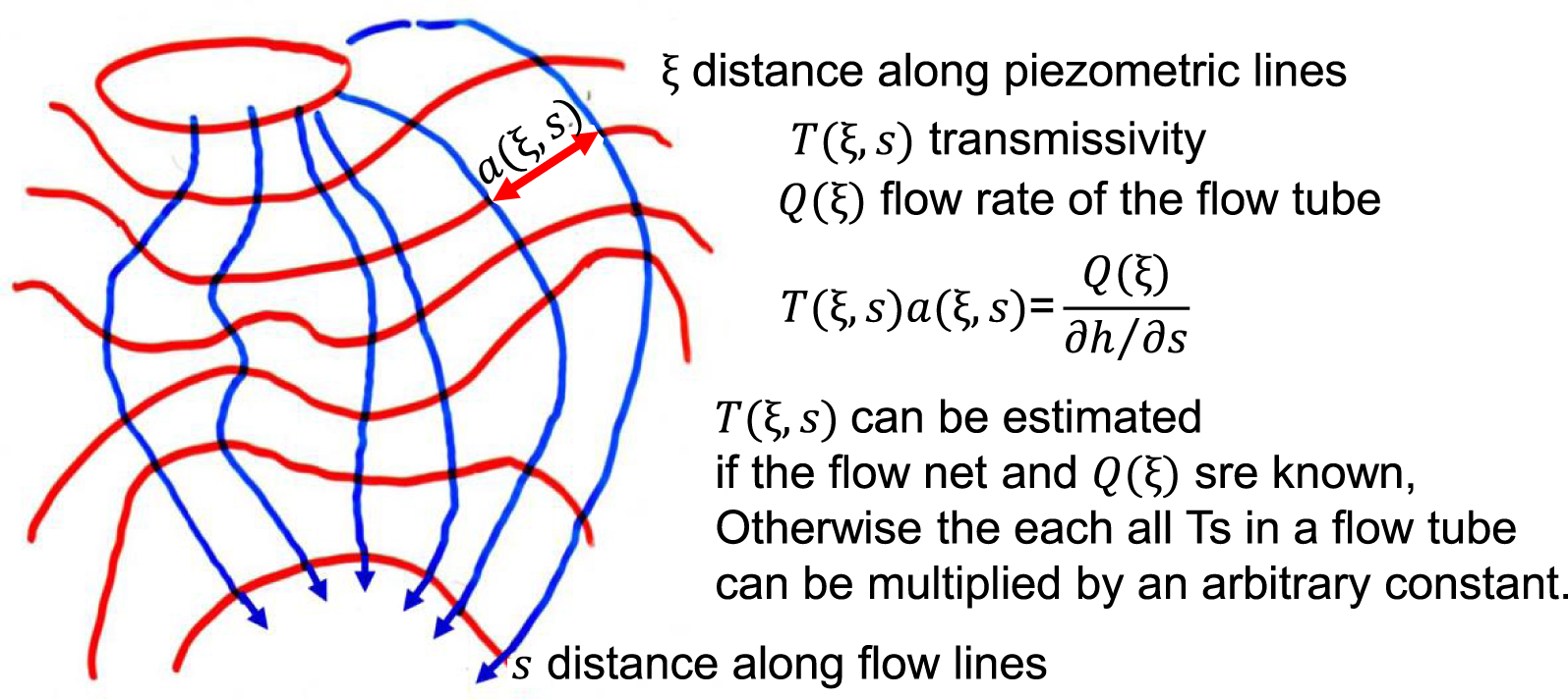
Early formulation of the inverse problem as integration of the flow equation along streamlines (picture taken from a lecture of GdM on the topic).
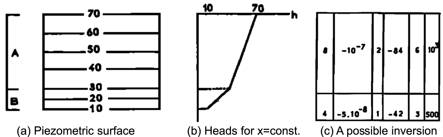
Example of Emsellem and de Marsily [1971] to illustrate the non-uniqueness of the inverse problem: (a) a medium with homogeneous T zones A and B (A twice as transmissive as B), will yield a piezometric surface with (b) twice head gradient in B than in A. Any T field as in (c), with along vertical lines TA = 2TB, will reproduce heads exactly [modified from Emsellem and de Marsily 1971].
To overcome these difficulties, Emsellem and de Marsily [1971] raised and then did three things that would mark future developments:
- The need for regularization. Since the solution can lead to arbitrary jumps, one should adopt a “smoothing” criterion to reduce arbitrariness, while ensuring existence and stability of the solution (i.e., regularization).
- The need for data other than heads to ensure resemblance to the actual aquifer i.e., prior information and adequate parameterization.
- To propose a general solution method based on minimizing mass balance errors when selecting the T field. While their method still required a full knowledge of heads, it was generalized in that it could be applied to transient problems with internal sinks and sources (even if uncertain). The full knowledge of heads may sound arbitrary nowadays, but one must bear in mind that automatic interpolation was not a standard tool in the 1960s. Therefore, hydrogeologists were used to draw piezometric surfaces with hydrogeological criteria, so that a good deal of conceptual understanding went into these maps.
These concepts marked future developments. The need for regularization was explicitly incorporated by Neuman [1973], who did two things. First, he formulated the problem in terms of head errors (minimizing the sum of squared errors on heads), which he termed the indirect formulation of the inverse problem [see also Yeh 1975]. Second, he formalized the smoothing criterion so that inversion became a multi-objective problem, with a model error criterion (e.g., the sum of squared errors) and a plausibility criterion incorporating prior information. The work of many others followed this path. Statistical formulations of the inverse problem were the immediate next step [Neuman 1980; Kitanidis and Vomvoris 1983; Carrera and Neuman 1986a; Rubin and Dagan 1987, and many others]. These formulations allowed formalizing the regularization requirement as a statistical problem. The issues of existence and identifiability were formalized by Carrera and Neuman [1986b].
Still, the instability problem remained. To the point that the inverse problem of groundwater hydrology was purported to be intrinsically unstable [Yakowitz and Duckstein 1980], i.e., a “morally ill-posed” problem. A large part of the problem rested on trying to estimate T everywhere. The discussions above (and the examples in Figures 1 and 2) make it clear that trying to estimate T(x) for all locations x within the domain will lead to an ill-posed problem, even if h(x) is accurately known everywhere. Since flow through permeable media is essentially dissipative, heads do not contain sufficient information about the small scale variability patterns of hydraulic conductivity. This feature motivated regularization methods, which initially were seeking smoothness. Obviously, nature is not necessarily smooth and a smooth solution does not need to resemble natural variability, which may become essential to other problems (notably, solute transport). Additional information on the nature of spatial variability is needed. Therefore, Emsellem and de Marsily [1971] sought expressing T(x) in terms of a number of parameters, while resembling natural variability. Note that, in doing so, the inverse problem moves from parameter estimation to model identification.
3. Parameterization
The problem of expressing the complete transmissivity field in terms of a (hopefully small) number of scalars is termed parameterization. The immediate option is to divide the aquifer into “zones” based on geological understanding. And this is still a basic option. However, this approach encounters numerous difficulties, from both theoretical and practical points of view. Geology is usually ambiguous, so it is not easy to define geological units accurately. Even if this was possible, geological units are not homogeneous.
A proper framework to study spatial variability is geostatistics, the study of random fields, which was introduced by Matheron [1967]. Two geostatistical tools are relevant to our problem. The first one, kriging, solves the problem of estimating a random function at a location, given measurements elsewhere. Since T(x) is generally assumed to be log-normally distributed, it is best to work with Y (x) = lnT(x). Then, the estimate of Y (x) at a location x, assuming that its values Yi are known at a set of measurement points xi is:
| (3) |
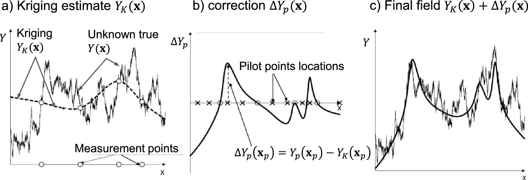
Schematic description on the pilot points method (PPM). (a) Kriging honors measurements but not variability away from measurements. (b) The PPM can be viewed as a correction of kriging estimation that can yield (c) adequate large scale variability (conditional simulation, instead of kriging, can be used for small scale variability).
3.1. Zonation parameterization
Zonation was the first parameterization strategy used for parameter estimation. It consists in partitioning the complete domain into zones where the parameter variability can be described by the same model (uniform value, statistical properties, etc.). The most common zonation for parameters is based on uniform values over a given subarea, but varying between diverse subareas. Pioneer works on zonation can be found in Jacquard and Jain [1965], and Jahns [1966]. In the work by Jahns, the inverse problem was solved using a regression problem (minimization of an objective function with a Gauss–Newton algorithm) based on a cost function as the quadratic norm of the vector of residuals (i.e., the squared difference between computed and measured heads). The number of zones was increased during the identification procedure and the reliability of the parameters was discussed in detail, addressing non-uniqueness due to Lorentz reciprocity in flow [see, e.g., Delay et al. 2011; Marinoni et al. 2016] and correlations between parameters. Jahns [1966] provided also computation times: 20 min for the estimation of 10 parameters with a 20 × 20 grid and 25 time steps.
Emsellem and de Marsily [1971] suggested adding a regularization term to the objective function by introducing a “smoothing” term in the minimization procedure to reduce the number of possible solutions. Adaptive parameterization was also described by successive refinements of the initial zonation. To our knowledge, for the first time, parameterization was embedded in the minimization procedure by adding to the cost function the quadratic norm of the transmissivity vector multiplied by a weighting coefficient. In this way, the parameterization was automatically accounted for in the inversion through the minimization procedure. Zonation can also be different for the same inverse problem, according to the type of sought parameters. For example, Zhang et al. [2014] proposed two different zonations for transmissivity and for elastic and inelastic specific storage parameters.
The main drawback of a raw zonation technique is the prior definition of the number of zones and their shape. The number of zones can be increased step-wise as suggested by Jahns [1966] and Emsellem and de Marsily [1971]. Carrera and Neuman [1986a], and Sun et al. [1998] also suggested some metrics to estimate the potential benefits of increasing the number of zones. These metrics were also used by Tung and Tan [2005] with a zonation based on Voronoï diagrams.
Several methods have been developed during the last twenty years to adapt the shape of the zones and the parameter values. Ben Ameur et al. [2002], Grimstad et al. [2003], and Hayek and Ackerer [2006] suggested the calculation of refinement indicators for the definition of the shape and the number of zones. Transmissivity is assumed to be a piecewise constant space function and unknowns are both the transmissivity values and the shape of the zones. The shape of each zone is adapted by relying upon refinement indicators easily computed from the gradient of the cost function. These refinement indicators define where to split a zone, rendering then the largest reduction in the cost function after the corresponding estimation. Level-set corrections were suggested by Lu and Robinson [2006] and Berre et al. [2007], for example, to deform the boundaries between zones to obtain a better zonation. The local deformation of the boundaries is proportional to the permeability contrast between the two sides of a boundary, the sensitivity of heads to transmissivity, and the residual between the simulated and observed heads.
3.2. Pilot points parametrization
Kriging represents the BLUE (Best Linear Unbiased Estimator) of Y (x). Therefore, a natural parameterization consists of extending the kriging equations (3) beyond the original set of measurement points, xi, by adding a set of pilot points, xp. The kriging estimate becomes:
| (4) |
A second difficulty in the original form was that pilot point estimates were not regularized, which caused instability and led modelers to emphasize both a “prudent” increase in the number of pilot points, and to bound the values of estimated Yp. Doherty [2003] included a regularization criterion penalizing non-homogeneity of the model parameters, while not using prior information [see details by Doherty et al. 2010]. Neglecting prior information results from viewing regularization in a “strict” Tikhonov sense (recall discussion on Tikhonov regularization in the introduction). As a consequence, limiting the number of pilot points remained a barrier and, for a while, it seemed that the method of choice was the self-calibration approach of Capilla et al. [1998] and Gómez-Hernández et al. [1997], which was able to reproduce quite accurately complex fields. The problem with the traditional formulation of the PPM was that direct measurements were used for the first term of (4), but were disregarded during the inversion process. Alcolea et al. [2006] overcame this problem by formulating the PPM in a fully geostatistical form. They explicitly acknowledged that pilot point estimates were part of the random field, which led naturally to a regularization term without any additional assumption. This formulation also allowed demonstrating that a stable inversion was possible, regardless of the number of pilot points, provided that a rigorous statistical formulation was adopted. In fact, Kitanidis and Vomvoris [1983] had already shown, via linearized co-kriging, that the number of parameters is not the real issue, but consistent geostatistics is. An additional advantage of the geostatistical formulation of the PPM is that it leads naturally to conditional simulation techniques, which is advantageous when one is interested in reproducing small scale variability [Lavenue et al. 1995].
A great advantage of the PPM is the ease with which complex problems can be addressed, which coupled with the flexibility of PEST software [Doherty et al. 2010], has allowed an explosion of the method in several directions. The PPM has been used with all kinds of equations and phenomena beyond groundwater flow [e.g., Vesselinov et al. 2001]. It has also been used in moments equation inversion [Hernandez et al. 2003], for fractured media [Lavenue and De Marsily 2001], or for multi-point geostatistics [Gravey and Mariethoz 2020; Ma 2018]. In short, the PPM has become the standard for non-linear geostatistical inversion. More details about PPM can be found in White and Lavenue [2022].
Nevertheless, a practical problem with the traditional PPM lies on its reliance on the geostatistical assumptions. It is clear that the PPM can lead to fully consistent and stable solutions. The question is whether the usual geostatistical assumptions provide good representations of geological variability. For example, the traditional multi-Gaussian paradigm was challenged by Gómez-Hernández and Wen [1998], who suggested that high transmissivity regions tend to be connected, which has repeatedly proven right. For example, Pool et al. [2015] compared the PPM (assuming stationary multi-Gaussian) to zonation on the basis of a simple geological model (paleo channels connectivity). They found that, while the PPM led to better calibrations (smaller calibration errors), geological zonation was better at predicting seawater intrusion. The implication is that traditional geostatistics is not sufficient and that proper incorporation of geological understanding is needed.
3.3. Parameterization based on geophysics
The use of geophysical methods such as electrical resistance tomography (ERT), seismic and radar transmission are expected to provide complementary data related to both the hydraulic parameter values in the subsurface and their spatial distribution. Measurements are done from the soil surface and are cheaper than traditional hydrological measurements such as pumping tests, which require “intruding” in the subsurface via wellbores. Furthermore, the acquisition of geophysical signals can be fairly well extended over the whole aquifer, which may prove helpful in tackling two main problems plaguing parameter identification for hydrogeological models:
- The representative volume of the measured transmissivity. This volume ranges from laboratory scale to pumping tests scale in hydrology. It is rarely consistent with the elementary modeling scale at which data should be estimated to document the cell/element scale of the model grid;
- The improvement of parameterization. The geophysical investigations should provide numerous images/patterns/values of geophysical parameters, assumed to be somehow correlated to hydrological parameters.
In short, the additional information from geophysics is expected to reduce the number of possible solutions, or at least permit sorting the “hydraulic” solutions that are in good stands with the subsurface structure evidenced by geophysics.
De Marsily and co-workers nicely highlighted the contribution of electric resistance measurements to the estimation of transmissivity. Ahmed et al. [1988] used the co-kriging of measured transmissivity, specific capacity, and electrical resistivity to elaborate transmissivity maps. They underlined that the contribution of electrical resistivity to transmissivity evaluation was important, but the diverse variables should be measured at a significant number of common locations to infer reliable cross-variograms.
The use of geophysical data in hydraulic parameter estimation was also addressed by Rubin et al. [1992], who combined head and hydraulic conductivity measurements at wells with a well-known seismic velocity field. Following the same approach, Copty et al. [1993] analyzed, in hydraulic parameter estimations, the effects of measurement errors concealed in the seismic velocity values. In their parameter estimation procedure, Dam and Christensen [2003] included the parameters involved in the relationships (state equations) between hydraulic conductivity and geophysical properties. They also used PPM for parameterization of both geophysical and hydrological parameters.
For these three approaches, the relationships between geophysical data and hydraulic conductivity were supposed to be known, although these relationships can be complex, often highly non-linear, and varying over space. Hyndman et al. [1994] circumvented this downside by using seismic data to delineate the geometry of lithologic zones. The hydrodynamic parameter values were then estimated for each lithologic zone by minimizing the sum of squared residuals between measured and computed tracer concentrations.
Haber and Oldenburg [1997] developed the joint inversion as a generic approach to invert two data sets when the underlying models are linked by the same structural (geological) heterogeneity. The main advantage of this approach is that it does not need any assumption about the relationship between the two data sets. Cardiff and Kitanidis [2009] showed the interest of the joint inversion via an adaptive zonation approach based on the level-set method. Finsterle and Kowalsky [2008] performed the joint inversion of ground penetrating radar (GPR) travel times and hydrological data collected during a simulated ponded infiltration experiment. Joint inversion is nowadays widely studied in hydrogeophysics [see Linde and Doetsch 2016, for a review].
In the field of hydraulic parameter estimation partly relying on geophysical data, the work of de Marsily and co-workers can be considered as seminal in initiating a promising research field leading to a new discipline, hydrogeophysics.
3.4. Parameterization based on lithological models
Solving the groundwater flow inverse problem has also been applicable in pre-conditioning the inversion by prior guess on the structure of the heterogeneity in the subsurface. When the structure is that of the spatial distribution of hydraulic parameters, for example, a correlated random field, the preconditioning is similar to a regularization technique, prescribing an overall distribution of hydraulic conductivities. Inversion and post-conditioning onto hydrological data can be carried out to add a perturbation to the prior parameter field [e.g., Ramarao et al. 1995].
However, there exist many geological contexts, in which a smooth field of parameters is not likely to represent the subsurface geological heterogeneity. In these contexts, the simulations of diverse “facies” distributions have revealed a better option. Geostatistical techniques contributed to this task by relying upon truncated Gaussian simulations [e.g., Matheron et al. 1987] or indicator sequential simulations [e.g., Schafmeister and de Marsily 1994]. In short, both techniques come down to calculate the probability of occurrence of a given geological facies at each location of the modeled domain. Nevertheless, the two-point covariance used to simulate the distribution of these probabilities and to avoid building a fully random “salt and pepper” image, still renders relatively continuous representations. These representations would not match the forecasts of geologists for complex systems such as fracture fields or sedimentary facies distributions in the subsurface of river floodplains. However, it is worth noting that improving the geostatistical methods, especially in developing truncated multi-Gaussian simulations and non-stationary random functions, renders to this day more realistic images [e.g., Beucher and Renard 2016].
In answer to the question of modeling with less pain the complex heterogeneity of the subsurface compartment in floodplains, G de Marsily and his co-workers elected models of sedimentation, in the form of a “genesis” model. Those are geared towards simulating the mechanisms that sequentially occur over time to build the floodplain. Tetzlaff and Harbaugh [1989] produced, via simplified equations of flow and transport, a model simulating river floodplains and deltas. This model was amended by Kolterman and Gorelick [1996], and employed to produce a reference work simulating the sedimentation over 600,000 years occurring at the east coast of the San Fransisco bay. The exercise was conditioned by a detailed history of climate forcing and needed very heavy computations.
The genesis model built by de Marsily and co-workers [de Marsily et al. 1998; Teles et al. 2001, 2004] relies upon empirical rules to move, as random walkers over a grid, elementary parcels of sediments. The rules are inherited from the literature in fluvial geomorphology, and adapted as a function of the successive dynamic episodes that construct the floodplain, mainly: braided systems, meandering, and channel incision. These episodes, even though not well documented for precise hydrodynamic conditions, can be detected and dated along the history of the river by log samples and geomorphological considerations. Parcels of sediments are of regular parallelepiped shape, the size of which depends on the type of sediment conveyed. The variety of sediments encountered in floodplains is simplified into a few classes, e.g., gravels, sands, and loam, to keep some relative continuity in the deposited sedimentary bodies, and avoid complex images that sometimes could resemble patchworks.
The genesis model was used to reconstruct parts of sedimentary floodplains of the Rhône and the Aube rivers (France). In the application to the Aube river, the structure modeled by the genesis model was compared to a model of facies build via the sequential simulation of indicators. For both models, facies were assigned hydraulic parameters values and forward simulations of flow and solute transport were performed. Regarding flow, both methods render very similar results in terms of hydraulic head distributions. It is worth noting that the flow scenario in the system is strongly conditioned by boundary conditions, and that piezometric heads are “robust” to parameters in the sense: it needs an important variation of hydraulic conductivity (or hydraulic diffusivity) to generate a small variation in heads. As both models, genesis and indicators, generate very different patterns of hydraulic conductivity distributions, the results pose the question of the identification of conductivities on the basis of heads only. Regarding transport results, simulations from both models do not match up at all. Transport (advection), is very sensitive to the flow patterns, both in terms of paths followed by the solute and concentration arrival times. The genesis model with its tortuous channels of high conductivity, guides transport through a few rapid pathways. For its part, the indicator model distributes more evenly the hydraulic conductivity values, with a consequence on transport of more widespread (diffuse) pathways with slower velocities.
In view of the above results, it goes without saying that parameterizations of the inverse problem inheriting from the geological structure of the subsurface are worth a try. Inferring or conjecturing this geological structure can be carried out via near subsurface geophysical investigations, process-imitating models (genesis models) and/or structure-imitating models (geomodels). At least, “geo-modeling” in its broad sense could open the equally probable solutions to an inverse flow problem, to solutions more convincing regarding the structure of the subsurface. To date, applications of geomodels find their way in engineering geology [Fookes et al. 2015]. With regard to hydrogeology, regional aquifers in sedimentary basins are often targeted [e.g., Ross et al. 2005], in almost the same way as for oil reservoirs or subsurface repositories. The geological model is usually aggregated at a scale rendering flow calculations tractable, and in this up-scaling process, the geological facies are directly transformed into a prior guess on hydraulic parameters. Along this line, the procedure looks like a pre-conditioning of inversion exercises on the basis of geological information.
It must be acknowledged that “genesis” models, including one developed by de Marsily and co-workers, did not receive much attention from the hydrological community. Nonetheless, modeling the floodplain construction continued to evolve, mainly for the purpose of simulating and predicting the geomorphological evolution of fluvial corridors [Williams et al. 2016]. Models mimicking either meandering [e.g., Pittaluga et al. 2009] or braided morphodynamics [e.g., Williams et al. 2016] continue to rely upon both a physically-based approach, solving flow and transport [e.g., Sun et al. 2015; Olson 2021], or on conditioned empirical rules [for example, automata cellular, e.g., Coulthard et al. 2007]. With the easier access to high-performance computing resources, the physically based models tend to overshadow models based on empirical rules.
4. Conclusions
Inverse modeling is widely used today. Regularization, incorporation of prior information, and parameterization in inverse methods are an art required for philosophy and a lot of conjectures, i.e., mathematical statements that are accepted as valid, but whose validity have never been proven or disproven. These conjectures are supported by plausible reasoning [Polya 1954] based on skills, training, and imitation. The most popular conjecture in inverse methods has often been: “Simplex sigillum veri”—simplicity is the sign of truth. This conjecture is now heavily discussed because inverse methods are nowadays not only developed for parameter estimation but also for improving model predictions by quantifying model uncertainty. With the increasing complexity of models, inversion strategies should focus not only on the number of parameters, but also on the smallest possible uncertainty, and in that case, the principle of parsimony may not hold [Gómez-Hernández 2006].
When applying inverse methods for parameter identification, several problems come up:
- The existing data sets can be complex and include measures of different support volumes, of different nature, with data spanning a broad range of numerical values, and that are more or less “hard” or “soft”, more or less “certain” or “uncertain”. Properly handling these data becomes an important step in the definition of the model concepts (physical processes taken into account, initial and boundary conditions, sink/source terms, etc.) and linked to the objectives of the model.
- The general design of the inverse procedure can be either deterministic or stochastic (Gaussian, multi-Gaussian) or both [Pool et al. 2015].
- Additional information (also called multiple source information) on the forecasted parameter structure inheriting from geological and geophysical data should be used as model constraints. This structure may be adapted (automatically or not) during joint inversion.
- The parameterization should be consistent with the design and the information on the parameter structure. It should limit the number of parameters (degrees of freedom) to be identified by using discrete locations (nodes, pilot points, master points). These locations should be defined in an “appropriate way” and their number increased during the inversion procedure, while keeping in mind that there exist techniques and indicators limiting useless parameterization [Hassane et al. 2017].
- Parsimony “as simple as possible, but not simplistic” is a good criterion to calibrate the model for specific situations i.e. when the variables lack sensitivity to the parameters (transmissivity estimation for a 2D flow model for example). However, it is not sufficient to address model uncertainty. Addressing model uncertainty, often quantified by parameter distributions and variances, needs the exploration of the ensemble of the plausible solutions [Moore and Doherty 2005; Ackerer and Delay 2010; Schöniger et al. 2012].
Research activity tackling the above-mentioned key features has concentrated on how to address regularization and to include prior information as a way to reduce instability of the inverse problem, including: geostatistical or deterministic methods to address spatial variability, and variants of PPM to parameterize this variability. Parameterization is now conditioned by geophysical data and/or lithology coming from field observations or lithology modeling. All these topics were introduced or addressed in the hydrogeological literature by Ghislain de Marsily. As in many other hydrogeological topics, he did not quite solve them (no one did it!), but, as “Tom Thumb”, he marked the path that many of us still continue to follow.
Conflicts of interest
Authors have no conflict of interest to declare.
Acknowledgments
Dr. Ackerer and Prof. Delay gratefully acknowledge the guidance of the young, yet wise, Prof. Carrera. Prof. Carrera thanks the co-authors for their contribution that will pave his future research during at least the next 20 years.