


 CC-BY 4.0
1. Introduction
The temperature of groundwater is a potential tracer of circulation that can provide insights into the dynamics of hydro-geological processes. When the pattern of the groundwater flow is diffuse, either through small pores of the rock matrix or through multiple fractures, the concept of representative elementary volume (REV) in porous media offers a conceptual framework for describing the heat and mass flow [de Marsily 1995, p. 12, p. 42]. In such a REV, the water fluxes are described by an average quantity (the specific discharge or Darcy velocity) and the thermal state of the rock-water system is characterized by a single temperature. In sedimentary basins, heat transfer in porous media explains satisfactorily the temperature field associated with large scale groundwater flow [Toth 1963; Smith and Chapman 1983]. Inversely, very deep temperature data, obtained in oil exploration boreholes for instance [Deming et al. 1992; Vasseur and Demongodin 1995; Reiter 2001; Pimentel and Hamza 2012; Tavares et al. 2014], are currently used to constrain the large scale underground flow in deep aquifers or to derive the field of permeability [Saar 2011]. In area of high geothermal potential, such as the Snake River Plain (USA), temperature profiles in boreholes and temperature gradients are useful to decipher the underground flow pattern and to infer its geothermal potential [McLing et al. 2016; Lachmar et al. 2017]. Alternatively, they can be used to estimate the area of the recharge [e.g. Ingebritsen et al. 1989].
In contrast with diffuse type water flow, in karstic aquifers, heat (and fluid) transfer cannot be described simply by transfer in porous media because a major component of the porosity is composed of very large pores and open channels. These conduits are focusing the initial slow water flow of the surrounding fractured medium and present very active flow following the laws of hydraulics. In fact, the surrounding rocks which provide the water recharge toward the localized conduit flow [Atkinson 1977], can generally be modelled as a porous medium; but inside the conduits, the water fluxes are best modelled by a network of pipes embedded in a porous rock matrix. Hybrid models have been used to simulate the transport of heat and reactive solute transport in coupled porous media and conduits [Liedl and Sauter 1998; Liedl et al. 2003; Birk et al. 2006; Covington et al. 2011] using mathematical and numerical models.
Many observations show that, when observed elsewhere than directly in karst intersections, the vertical gradient of temperature in karstic areas is generally much lower than expected [Mathey 1974; Luetscher and Jeannin 2004]. This suggests that a large proportion of the regional geothermal heat flow may be captured by the water flow and eventually warms the out-flowing waters. Quantitative studies of heat flow processes within the saturated zone of karst systems are available [Benderitter et al. 1993; Lismonde 2010; Badino 2005]; these studies are mainly based on the temperature of the karstic conduit whereas the quantitative understanding of the physical interaction between the water flow and the heat flow requires to account not only for the temperature within the conduit, but also for the temperature field inside the surrounding rocks.
This study develops an analytic model describing the temperature field in a system based on the conceptual model of fluvio-karst described by White [2002, 2006]. This model is applied to the actual karstic zone of the Lez spring where a series of thermal data are available. The underground system of the Lez spring, located about 15 km North of the city of Montpellier, is a classical example of “karst barré” [or “damed karst”, Bakalowicz 2005]; it gives birth to the Lez river which ends southward in the Mediterranean sea (28 km length). The watershed area feeding this spring has had relatively low structural deformation: the geometry of the corresponding underground karstic system is not directly known but it is likely to be relatively horizontal as is the general stratification. The Lez karstic network may thus be considered as a convenient example of underground sub-horizontal conduit.
The generic hydrological model used is illustrated on Figure 1 and is inspired from Ewers and Quinlan [1985]: rain infiltrates in the fractured medium, then merges toward a horizontal open conduit thereby contributing to the horizontal flux toward the natural outlet. Several simplifying assumptions are used: an idealized geometry is assumed and composed of a porous/fractured matrix connected to a horizontal conduit flow bounded by two horizontal planes as illustrated farther by Figure 8. The transverse dimensions of the conduit are small enough so that their internal temperature is nearly homogeneous. Following Bovardsson [1969] and Ziagos and Blackwell [1986] for open fractures—but also Vasseur et al. [2002] and Burns et al. [2016] for a thin horizontal aquifer instead of open conduit—the presence of such a horizontal concentrated flow can be accounted for through a specific boundary condition. This boundary condition, based on the energy and mass budget of the fluid system, is imposed on the limits of the porous medium. Only the steady state temperature is considered which implies that the actual recharge is simplified to an average constant rain. Moreover the porous medium is saturated and the fluid inside the conduit is assumed to be well mixed—or even turbulent—so that it is characterized by a single temperature. Using several other assumptions (mainly a very simple geometry of the flow and a negligible horizontal component of thermal conduction), it is possible to obtain simple analytical functions relating available hydrothermal data to a few hydrogeological parameters. This model is then applied to available observations of the Lez spring to obtain a better understanding of the interaction between the geothermal heat flow and the hydrological system.
Block-diagram inspired by Ewers and Quinlan [1985] showing the underground flow of water in karstic districts. The two types of water flow are illustrated in blue: slow infiltration in fractured rocks and relatively rapid flow in concentrated conduits.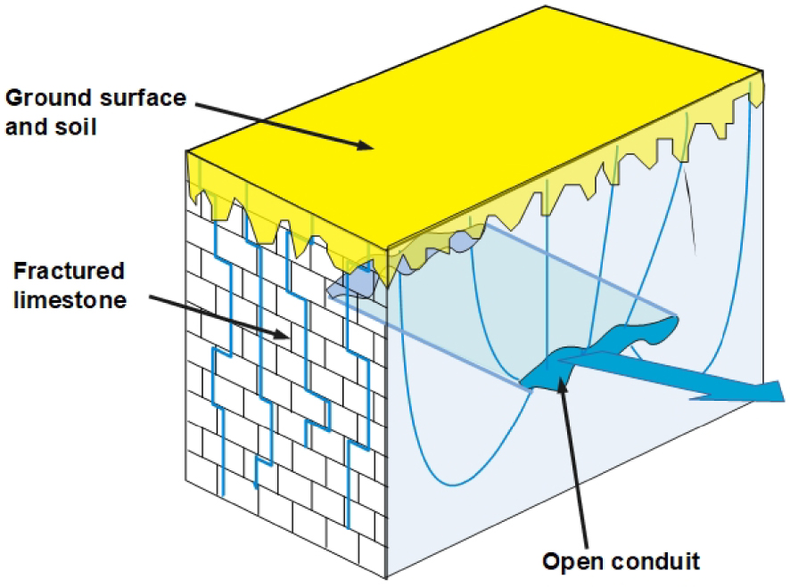
2. Presentation of the Lez spring system and of its geothermal context
The general context of the Lez spring system has been intensively investigated because it has been for a long time and is still the main source of drinking water for the urban agglomeration of Montpellier [Drogue 1969, 1985; Lacas 1976; Avias 1992, 1995; Guilbot 1975; Uil 1978; Bérard 1983; Botton 1984; Touet 1985; Karam 1989; Malard and Chapuis 1995; Dausse 2015].
2.1. General presentation of the system
The Lez karstic system belongs to the Mesozoic carbonate series of Languedoc which were deposited from Lias to Cretaceous on the north-western margin of the Tethyan Ocean, controlled by N-E trending faults such as the Cevennes fault (CF on Figure 2) and the Nimes fault (NF on Figure 2) [Husson 2013]. During Cenozoic times, several geological events have imprinted the area: the Eocene Pyrenean orogeny followed by the Oligocene rifting of the gulf of Lion imposed a drainage system flowing southward and a reactivation of fault systems oriented North-East. The result is a system of large faults (mainly normal to strike slip) in the North to North-East direction as well as thrusts trending in the East–West direction located North of the Montpellier city. The last transgression occurred during early Miocene followed by an uplift during which the base level falls of 1500 m. These episodes have sculpted a large karstic system in such a way as to adapt the drainage hydro-geological flow from mountains North of the Cevennes fault toward the Mediterranean sea to the topographic evolution [Avias 1992; Bakalowicz 2005; Husson 2013].
Simplified hydrogeologic map of the Languedoc karstic area with coordinates in km (Lambert 2 projection). The background illustrates the simplified geology: pre-Jurassic (basement to Lias) in pink, Jurassic in blue, Cretaceous in green and Cenozoic (Oligocene to Quaternary) in yellow. The thick lines are the main tectonic accidents: strike slip faults (FC for Cevennes fault, FM for Matelles fault and FN for Nimes fault) and overthrust faults are toothed black lines. The heavy blue lines show the main rivers (Hérault, Lez, Vidourle). The Lez spring is the red star and its recharge basin is shown by a dotted red line. The green square is for the Montpellier town, the symbol “v” for the Valflaunes meteorological station. The horizontal and the vertical orange scale bars present the limits in the EW and NS directions of the studied zone (restricted zone of Figures 3 and 5).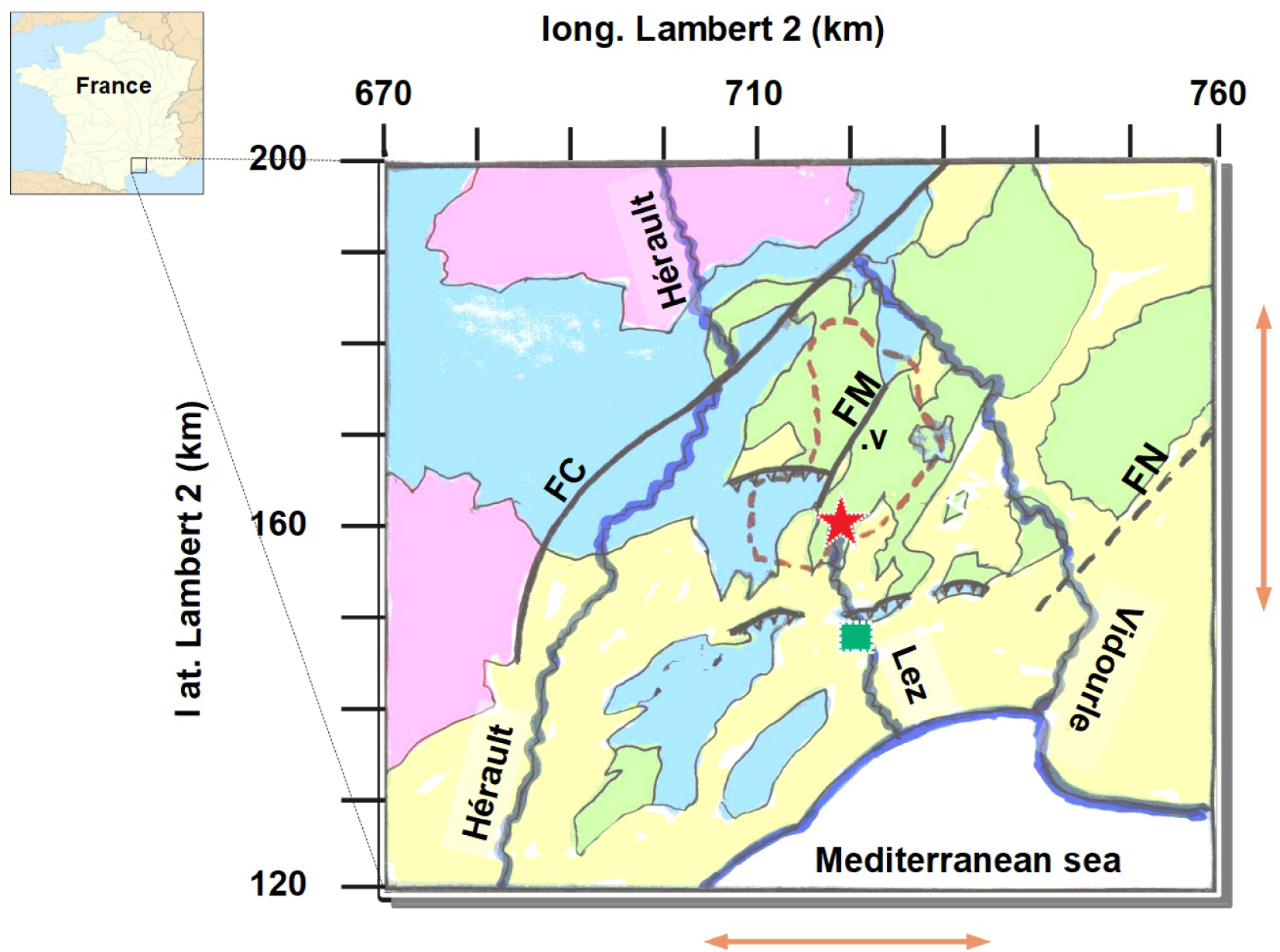
Location of the deep exploration boreholes in the western part of the South Provence basin where BHT temperature measurements are available. The green square is the town of Montpellier, the red star is the Lez spring and the red curve bounds its surface recharge. A restricted 35 × 30 km2 area around this recharge area is shown by a rectangular inset and corresponds to the range illustrated by orange arrows of Figure 2.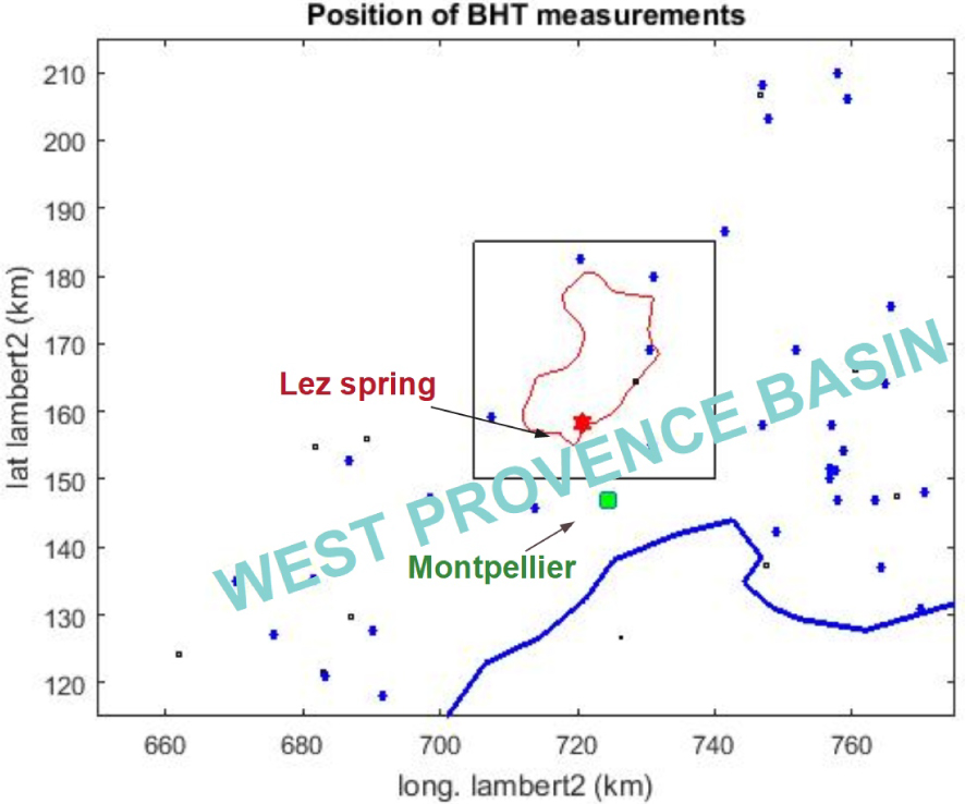
The watershed of the Lez spring is part of the karstic hydrogeological system called the North Montpellier Garrigue unit, delimited by the Hérault river (to the West) and the Vidourle river (to the North and East). The geological setting and the major tectonic structures characterizing this unit are illustrated in Figure 2 from CERGH [1978]. The karstic aquifer layer has an estimated thickness of 650 to 800 m within the Upper Jurassic layers on both sides of the Matelles Fault (MF on Figure 2) with a thick succession of Lower Valanginian (Lower Cretaceous) marls and marly limestones; the aquifer itself straddles in the Upper Jurassic and the Berriasian (Lower Cretaceous). The karstic conduit has been recognized by diving with a cross sectional width of a few meters at a depth of about 100 m, and was explored only in the vicinity of the spring; the general geometry of the network remains speculative as largely deduced from geological observations and hydrological measurements such as dye, piezometer, chemistry…. [Marechal et al. 2014]. Following a proposition by Dubois [1964] and using hydro-dynamical observations, Karam [1989] speculates on the existence of a single major karstic conduit running from North to South, along the major fault of “les Matelles” (“FM” on Figure 2). The major hydrogeological characteristics of the system have been summarized in Avias [1995]: with a natural overflow lying at 65 m (asl), the Lez spring is the main outlet of a large hydrogeological catchment; its area—illustrated on Figure 2—is estimated around 250 km2, based on geology, dye tracings, and groundwater level dynamics in the network of observation boreholes during the draw down [Ladouche et al. 2014; Thiery et al. 1983; Dausse 2015; Marechal et al. 2014]. Its recharge zones include (i) the Jurassic limestone outcrop (between 80 and 100 km2), (ii) the Cretaceous marly limestone formations through leakage toward the underlying Jurassic. Tertiary formations are generally impervious and contribute insignificantly to the karst aquifer recharge.
For more than 200 years, the Lez spring has been the main supply of drinking water for the city of Montpellier but the equipment for collecting the spring has evolved. Prior to 1968, the resource was exploited through spring overflow collection between 25 and 600 l/s [Paloc 1979], then from 1968 to 1982, through pumping in the pan hole at a rate of some 800 l/s. Following this period, a so-called “active management” of the Lez karst system was undertaken with pumping rates in the summer periods exceeding the natural discharge; from 1982, deep wells were drilled into the main karst conduit upstream of the spring in order to reach a maximum yield of 2000 l/s [Avias 1995] through pumping units.
2.2. Estimate of the average volumetric and energetic discharge
The natural volumetric discharge of the karst system is not directly observed, because the Lez spring has been tapped since 1854. However, its pumping rate has been measured since 1974 and the spring’s residual overflow discharges were reliably measured between 1987 and 2007. From these observations, the yearly flow is about 62 × 106 m3⋅y−1 which corresponds to a mean of about 2 m3⋅s−1. In fact, during floods, the instantaneous flow rate may exceed 10 m3⋅s−1; analyses of time series of water precipitation, flow rate and hydraulic head [Ladouche et al. 2014] emphasize the relatively inert behaviour of the system with respect to the infiltration of rain, since its characteristic time constant is on the order of 100 days.
A few records of the water temperature at the end of the spring (i.e. in the conduit itself) are available before the development of the underground pumping factory in 1982 [Lacas 1976]: the average temperature was around 15 °C with a slight seasonal variation: the temperature was nearing 17 °C during low-water summer and tending toward lower values of about 14.5 °C following strong rain episodes. With the new technical development of the spring tapping and pumping system, hourly records of the pumped water are now available from 2006 on; it appears that the temperature of the pumped water does still vary between 14.5 °C and 17 °C and is clearly anti-correlated with the pumped flow rate. For the present study, possible artificial effects associated with the recent technical developments are ignored and the period around 1980 is chosen as reference one, when most of the present data were acquired. For this time, the mean annual temperature of the discharging spring is estimated to 15.75 °C.
In order to obtain an energy budget of the karstic system, it is also necessary to assess the input temperature of the rain water. Meteorological observations are available at several locations of the watershed area [Thiery et al. 1983] providing monthly averages of precipitation and temperature. The average annual surface temperature is somewhat dependent on the altitude of the station varying from 14 °C in its lower part (altitude 65 m) to 12.5 °C in its upper one (altitude 200 m). The Valflaunes meteorologic station (altitude 135 m, station labelled “v” on Figure 2) located in the centre of the watershed has an average annual surface temperature of 13.5 °C. Taking into account the fact that most rainy events occur during equinoxes, the average temperature of the rain is assumed to be equal to that of this later representative station (i.e. 13.5 °C). Another argument in favour of this choice is obtained from vertical profiles of temperature obtained in near surface boreholes of the area: as shown by Touet [1985], when vertical temperature profiles in the 30–100 m depth range can be extrapolated toward the ground surface, the extrapolated ground surface temperatures lies in the range (12.75 °C–13.8 °C). A value of 13.5 °C is therefore assumed to be the average temperature of the ground surface (soil + water).
In conclusion, the average discharge temperature of the spring Tdisch = 15.75 °C is 2.25 °C higher than the assumed rain temperature (average Tinput = 13.5 °C). Taking into account the average flow rate of the spring (q = 2 m3⋅s−1), this implies that during its underground path the water flow has been receiving a mean energetic input Espring given in watts (W) by: Espring = (𝜌C)q(Tdisch − Tinput) = 4.18 × 106∗2.25∗2 W = 18.8 × 10⁶ W = 18.8 MW, where (𝜌C) is the volumetric heat capacity of water. It is reasonable to assume that this heat exchange process occurs at steady state. Obviously this energetic contribution is mainly provided by the geothermal heat flux.
2.3. Deep regional geothermal heat flow
Over continents, heat flow data are generally obtained from temperature profiles measured in boreholes with a few hundreds of m depth; in particular, heat flow maps of France [Lucazeau and Vasseur 1982; Bonte and Guillou-Frottier 2006] show that the area of southern Languedoc is characterized by a regional heat flow of 80 to 90 mW⋅m−2. An essential condition for obtaining significant heat flow data is to avoid areas where heat convection occurs through active water flow; this precludes the use of such temperature profiles in karstic areas. However in most sedimentary basins, the oil industry has been drilling very deep boreholes for hydrocarbon exploration, reaching depths (several km) where active hydraulic fluxes are certainly much smaller; bottom hole temperatures (BHT) are recorded during well-log acquisition, being imposed more by technical purposes than by scientific ones. These rough BHT data suffer of biases reaching 5 to 15 °C due to thermal perturbations during the drilling operations but these data can be corrected leading to a set of un-biased but noisy temperatures [Vasseur et al. 1985].
A recent compilation of these data pertaining to the Provence basin (South-East of France) has been published showing a relatively consistent pattern of the deep temperature field [Garibaldi et al. 2010; Garibaldi 2010]. For the present study, the analysis is focused on the western part of the Provence basin, i.e. west of 5 °E longitude and illustrated in Figure 3. The location of used wells (111 BHT data of which 89 at depth larger that 1000 m) is shown on Figure 3 together with a scatter plot of obtained temperatures versus depth on Figure 4. There is a clear linear increase of the temperature as a function of depth. The standard deviation (SD) of the departures between the linear fit and the data reach about 14 °C. The coefficients of the best square linear fit, with their SD writes as:
| (1) |
Plot of the measured BHT temperature versus their measurement depth (z) and best linear fitting lines. The left plot is for the whole area of Figure 3 and the blue line for best fit has equation T(z) = 13.5 °C + 0.0318z. The right plot deals with the restricted area of the inset of Figure 3 and the fitting line T(z) = 2 °C + 0.0.0304z, in red, is compared with the previous one of the whole area, in blue.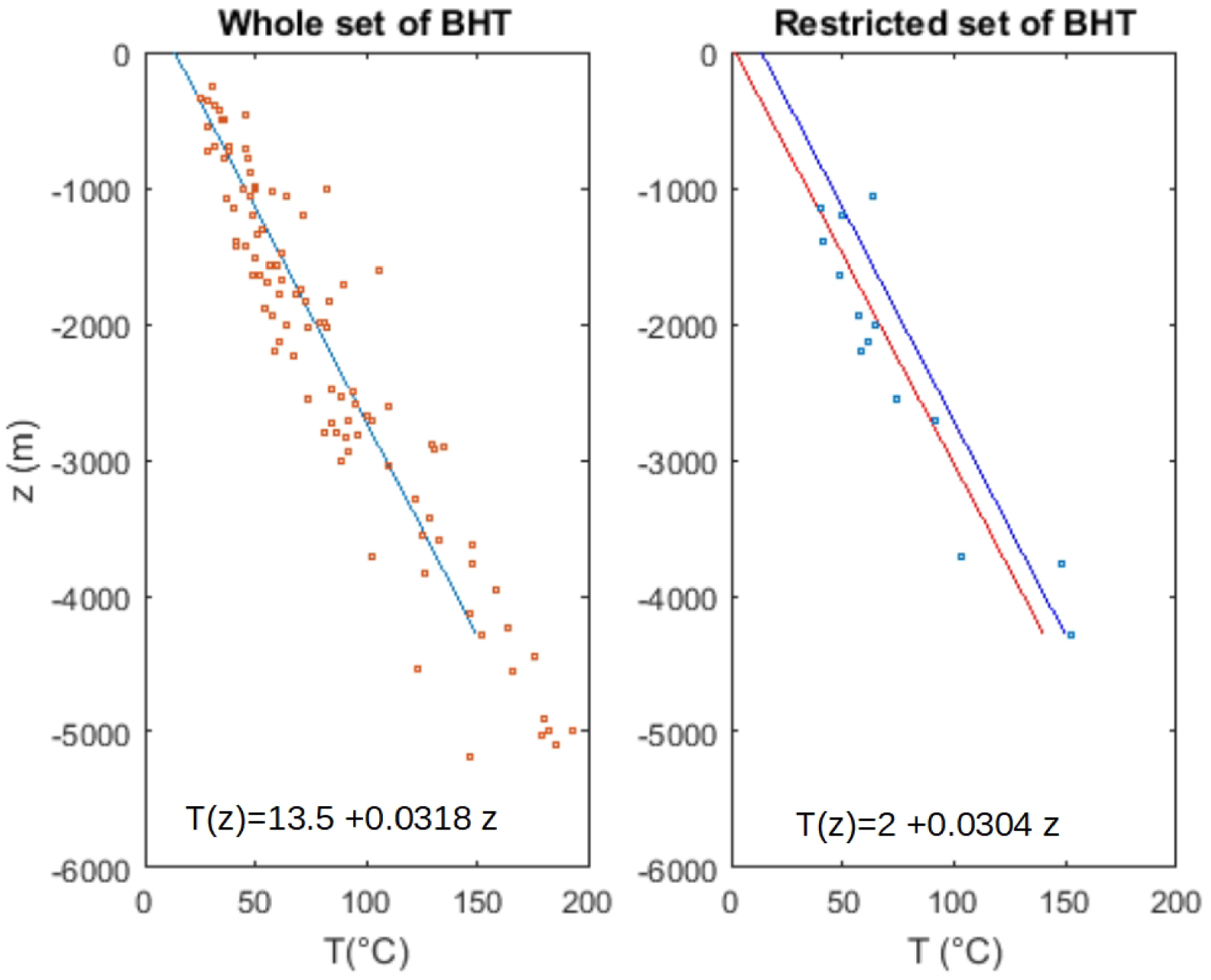
The value at the earth surface (13.5 ± 0.9 °C) agrees with the one previously estimated.
Figure 4 also presents the temperature versus depth plot for a more localized area covering the immediate vicinity of the catchment zone and implying a smaller number of data (14 BHT). When compared to the previous linear trend, most data plot at a significantly lower temperature; indeed the regression of these data gives the following linear trend:
| (2) |
It is clear that a mean regional gradient (𝛾= dT∕dz) of 0.031 °C⋅m−1 (or in practical units 3.1 °C/100 m) applies to deep temperatures in the zone of interest. With such a gradient, the regional basal heat flow—based on the assumption that conduction is dominating at great depth—can be evaluated as KdT∕dz where K is the average thermal conductivity. The formations encountered in the various boreholes are mainly composed of carbonates and dolomites of Jurassic and Cretaceous age. The thermal conductivity K of such rocks can be evaluated from its composition and porosity; following Brigaud and Vasseur [1989] a value K = 2.75 ± 0.5 W⋅°C−1⋅m−1 is assessed. Assuming that conduction dominates at depth at this regional scale, these values imply a regional heat flow KdT∕dz of about 85 × 10−3 W⋅m−2 in agreement with available heat flow maps of France [Lucazeau and Vasseur 1982; Bonte and Guillou-Frottier 2006].
Over the catchment area (∼250 km2), the integrated energy from this geothermal flux is:
| (3) |
To within experimental errors, this is very close to the mean energy Espring needed for heating the spring which was estimated above from independent data. Assuming steady state conditions, everything happens as if the geothermal flux was completely absorbed for heating the water flowing in the upper crust of the Earth and emerging at the Lez spring. This absorption can indeed be verified experimentally through available temperature profiles observed in shallow wells.
2.4. Shallow temperature gradients at basin scale
Many temperature profiles in relatively shallow boreholes of the studied area have been obtained in the 80s: Uil [1978], then Botton [1984] and Drogue [1985] obtained measurements in several boreholes 60 m deep located in the immediate vicinity of the spring. A wide survey at large scale was provided by Touet [1985] from high precision temperature profiles in several superficial boreholes 50 to 200 m deep located in various parts of the catchment. Most of these profiles have reached the homo-thermic zone (where seasonal effects are very small) and many of them present a clear linear trend as a function of depth. However some of these temperature profiles reflect local disturbances due to local fluid flow such as spikes due to occasional fast fluid flow across boreholes that are easily recognizable, or to flow along boreholes between two levels that is more difficult to detect.
A careful examination of these profiles allows sorting out those temperature profiles which present a regular linear trend versus depth—excluding profiles with spikes indicating lateral water arrival [Ge 1998; Vasseur et al. 2002]. Moreover these profiles should exhibit an extrapolated ground surface consistent with meteorological data. About 17 thermal profiles have been retained, the location of which is illustrated on Figure 5 together with their geological background and two interpreted seismic cross sections of the area. Figure 6 displays seven of these profiles obtained in 1983 by Touet [1985]. The temperature gradients are all lower than 3 °C/100 m (from 0 to 2.9 °C/100 m) with a mean value on the order of 1.2 °C/100 m; from their geographic distribution, it seems that smaller values (less that 0.9 °C/100 m) are obtained toward the centre and western part of the catchment whereas higher values (near 2 °C/100 m or above) are observed toward its northern, eastern and southern edges. A trend analysis of these data, fitted with a polynomial of second degree in x and y as shown on Figure 7 confirms this trend: a zone of depleted gradient occurs toward the centre of the recharge zone.
(a) Location of near surface thermal gradient data [Touet 1985] in their geological context [CERGH 1978]. The colour code is the same as for Figure 2. The Lez spring and the limit of the basin are shown in red and the dots represent the location of individual thermal gradients with their label. Open symbol are for thermal gradient <1 °C/100 m and filled ones for >1 °C/100 m. The triangle T is the location of Terrieu. Orange lines a–a′ and b–b′ correspond to available seismic profiles. (b) Two cross sections along approximate NS and EW directions obtained from migrated seismic data as interpreted by Husson [2013].
Illustration of seven typical near surface thermal profiles with corresponding thermal gradient 𝛾 = dT∕dz in °C/100 m. The profiles measured in 1983 are redrawn in red from Touet [1985]. The ordinate is the depth from the ground surface; the level of the water table is shown as a blue line and the number in square inset correspond to the label located on Figure 5.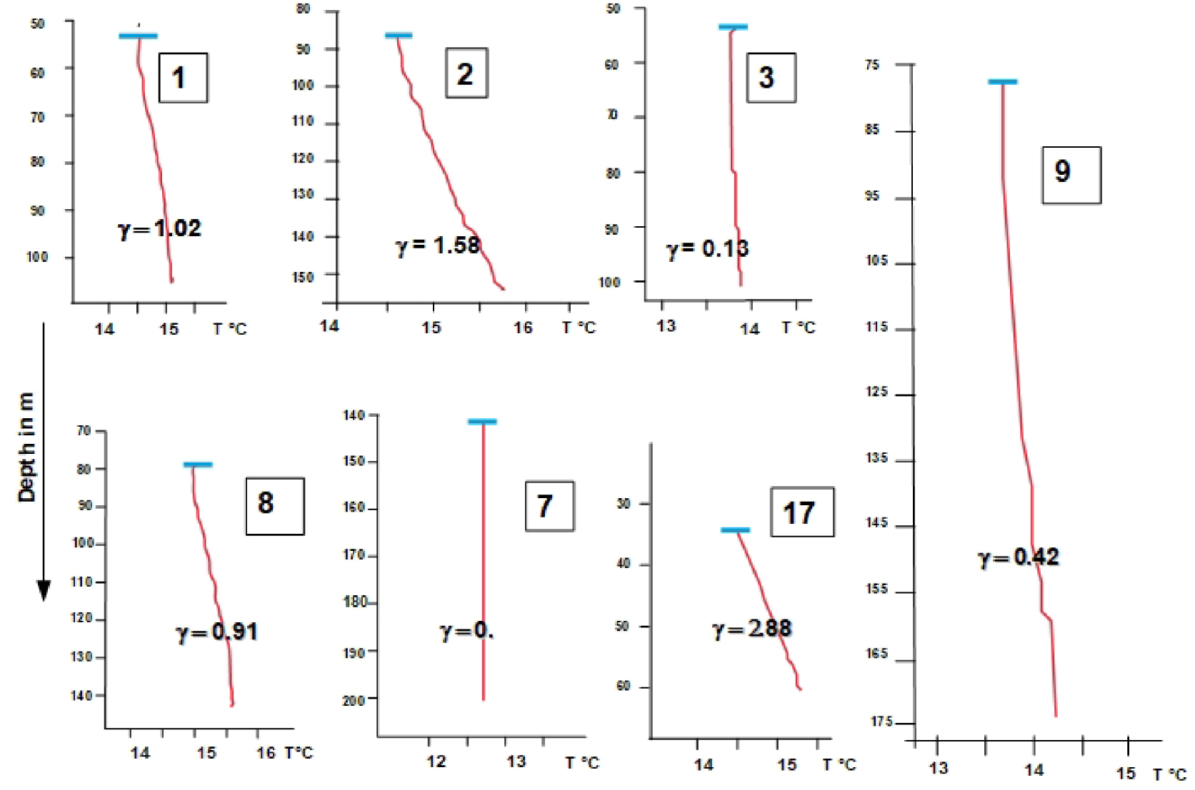
The large scale trend of the surface thermal gradient fitted by a polynomial surface of second degree in latitude–longitude on the same area as Figure 6. The values are in °C/100 m and the position of individual data is illustrated by dots. The size of dots is proportional to their value according to the bottom right legend (in °C/100 m).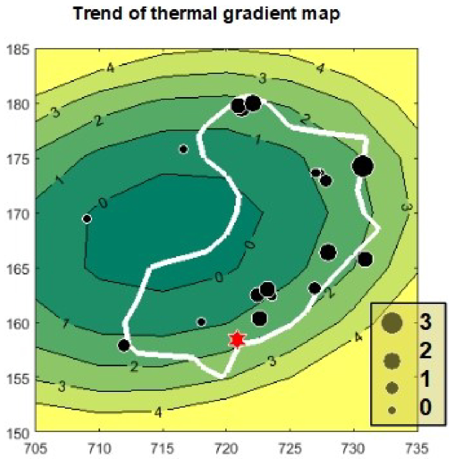
3. A simplified model of karst circulation
Based on the scheme described on Figure 1, a simplified model is designed where the karstic conduit, simulated by a horizontal fracture, is embedded in a porous medium simulating the fractured medium. This model, illustrated by Figure 8, reduces the problem to a pseudo 2-dimensional one and allows a simple analytical solution. Notations are summarized in Table 1.
Simplified geometry of the model used; the reference frame is Oxyz, Oz being the downward vertical, Oxy the ground plane (yellow) and Ox the direction of the conduit flow. The conduit is a thin horizontal fault of thickness 𝜀 at z = h. The water fluxes, illustrated by blue arrows, are vertical in the surrounding porous medium; they converge into the conduit to follow the Ox direction.
List of used symbols
| Symbol | Significance | Unit |
|---|---|---|
| C | Heat capacity of the water per unit mass | J⋅kg−1⋅°C−1 |
| E | Energy output | W |
| EE | Function defined by EE(u) = erfc(u)exp(u2) | |
| FS | Conductive heat flow at the ground surface | W⋅m−2 |
| G = g∕C | Thermal gradient associated with gravitational potential dissipation | °C⋅m−1 |
| H | Hydraulic head = p∕(𝜌g) − z | m |
| K | Thermal conductivity of porous medium | W⋅m−1⋅°C−1 |
| L | Length of the conduit (x direction) | m |
| Pe | Peclet number | |
| R | Radius of a horizontal disk | m |
| Sf | Shape factor | m |
| T(x,z),T+,T− | Temperature field in the porous medium, above h, below h | °C |
| T0,Tground,Textrap | Temperature in the conduit of the ground and extrapolated | °C |
| V | Specific discharge in z direction. Eventually vector (Darcy vel.). | m⋅s−1 |
| e | Specific enthalpy e = CT + p∕𝜌 | J⋅kg−1 |
| g | Acceleration of gravity (g = 9.81) | m⋅s−2 |
| h | Depth of the conduit | m |
| q | Horizontal flux in the x direction per unit y | m2⋅s−1 |
| x | Horizontal coordinate along the flow | m |
| y | Horizontal coordinate perpendicular to x | m |
| t | Time | s |
| z | Vertical coordinate orientated downward | m |
| 𝛼 | Vertical gradient of H | m/m |
| 𝛽 | Horizontal gradient of H | m/m |
| 𝜀 | Thickness of the conduit | m |
| 𝛾 | Geothermal gradient | °C⋅m−1 |
| 𝜌 | Density of water | kg⋅m−3 |
| 𝜅 | Diffusivity of the porous medium (𝜌C)r∕K | m2⋅s−1 |
| 𝜃 | Specific methalpy 𝜃 = e − gz | J⋅kg−1 |
| (𝜌C) | Volumetric specific heat of water | J⋅kg−1⋅°C−1 |
| (𝜌C)r | Volumetric specific heat of medium, of water | J⋅kg−1⋅°C−1 |
| 𝜏diff, 𝜏conv | Time constant for diffusion, convection | s |
3.1. Basic assumptions
The reference frame illustrated on Figure 8 is such that Oxy is the ground surface assimilated to the water table, Oz the downward vertical, and Ox the horizontal direction parallel to that of the water flow inside the conduit. In the porous rock matrix (0 < z < h), the porous water flow is characterized by the downward component of the specific discharge and its temperature T is in equilibrium with that of the rock.
The thermal energy is transported by conduction in the porous medium with an energy flux given by—K grad T (K being the thermal conductivity of the porous medium) and also by convection of the moving fluid. The total energy per unit mass transported by this moving fluid is composed of its thermal energy written as CT (C the heat capacity per unit mass) plus other types of energy: internal fluid pressure, kinetic energy and potential energy. The necessary introduction of gravity potential in the total energy budget of porous flow has been pointed out in several theoretical studies [Sposito and Chu 1981; Hassanizadeh and Gray 1980]. More recently Stauffer et al. [2014]—see also Burns et al. [2016]—have enlightened the subject in practical applications; following Stauffer et al. [2014], the methalpy 𝜃 sums up the specific enthalpy e = CT + p∕𝜌 (p being the fluid pressure, 𝜌 its density) plus its kinetic energy V2∕2 (in fact negligible in porous media) and finally its potential energy due to its evolution in the gravity potential i.e. −gz (z being directed downward). The methalpy is defined by:
| (4) |
| (5) |
| (6) |
Therefore, in the whole porous domain, the energy conservation in steady state conditions is expressed as:
| (7) |
| (8) |
At depth z = h, as shown on Figure 8, lies a conduit assimilated to a “horizontal feature” with vertical thickness 𝜀 (𝜀≪h). This feature is in fact associated with a hydraulically conductive structure which is stretched in the x,y directions. It could even be a thin aquifer much more conductive that the overlying medium; in the following it is referred to as “plane conduit”. Inside this conduit, the horizontal water flow q(x) is the cumulative result from the downward flow occurring in the overlying porous medium (vertical component V along coordinates z). At steady state, mass conservation imposes that the vertical specific discharge (Darcy velocity) is related to the increase along x of the water flow rate q (in m2⋅s−1 i.e. per unit length in the y direction) so that q and V are related by:
| (9) |
In the porous medium located above the conduit (z < h), the temperature field indexed as T+(x,z) is submitted to the downward water flow and from (7) satisfies the following equation:
| (10) |
| (11) |
Classical boundary conditions include imposed temperature at the ground surface (arbitrarily set to 0) and imposed vertical gradient 𝛾 (or given geothermal heat flux 𝜑geoth = K𝛾) at great depth, so that:
∙ at z = 0
| (12) |
| (13) |
At the level z = h, two specific boundary conditions are required: one accounts for the continuity of the temperature and the other for a possible discontinuity of its derivatives accounting for the energy conservation in the conduit. Since the thickness 𝜀 is very small, the temperature above and below are continuous (but not their vertical derivatives) so that:
∙ at z = h
| (14) |
∙ at z = h
| (15) |
Budget of mass and heat transfer in an elementary cell of the conduit illustrating the various components: the water fluxes are shown in light blue, the convective fluxes of heat content (𝜌C)T and gravity-head potential 𝜌gH in dark blue and the conducting fluxes in red.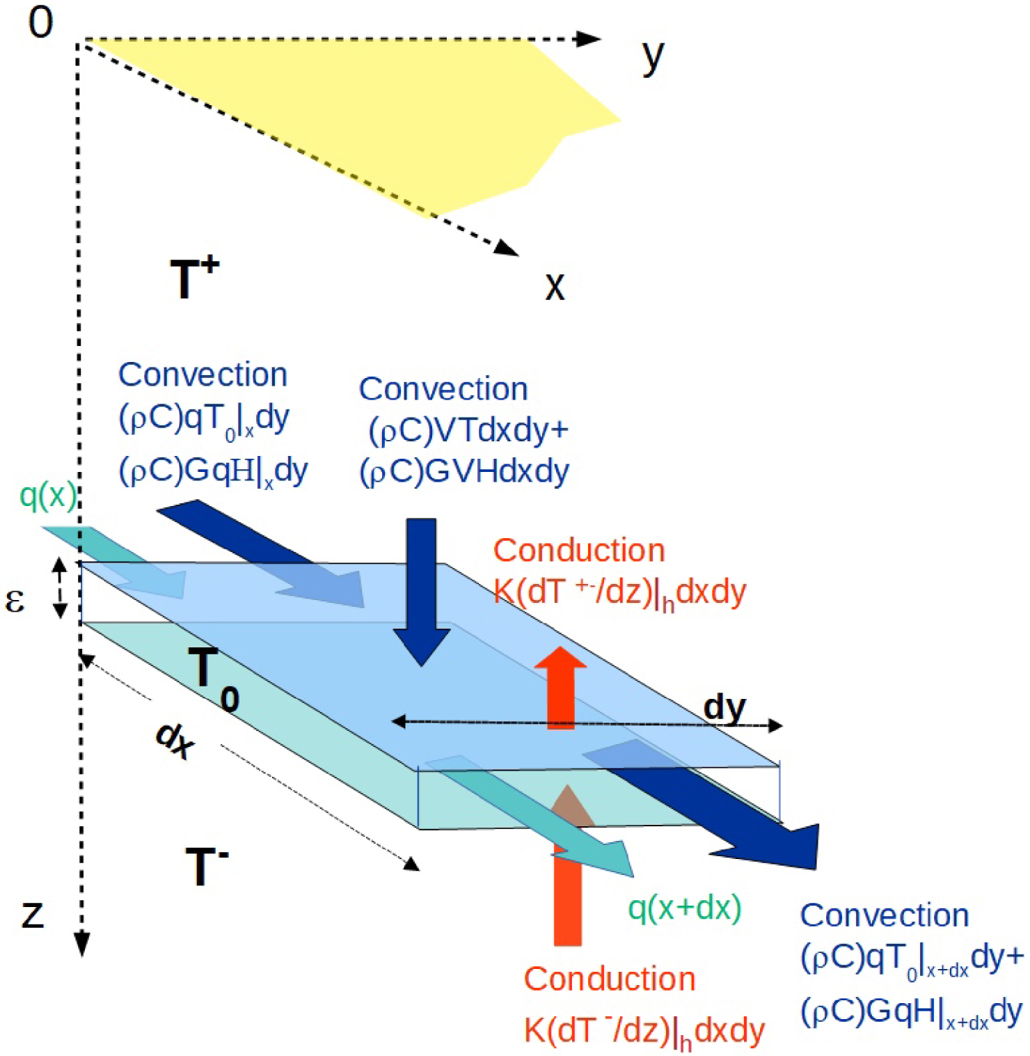
Since steady state is assumed, the energy budget of the conduit element equal to 0 provides the fourth boundary condition as (15). This boundary condition seems quite similar to the one stated by Bovardsson [1969], Lowell [1975], Ziagos and Blackwell [1986] for the case of a horizontal aquifer. In fact it differs because the energy contains more than internal heat as already stated by Burns et al. [2016]. But the main difference is that horizontal water flux q(x) is not constant with x: it is accumulating the water flux supplied vertically by the porous flow.
In the next paragraphs useful analytical solutions are obtained for cases where the parameters 𝛼 = −dH∕dz in the porous medium, and 𝛽 = −dH∕dx in the horizontal conduit are assumed to be constant on the whole domain. Both parameters 𝛼, 𝛽 are related the dynamics of the underground water flow along the path. Since the flow is orientated downward and toward the spring, 𝛼 and 𝛽 are strictly positive; This implies that −dH∕ds (i.e. 𝛼, 𝛽) acts as a positive energy contribution in (15). Moreover they belong to the range [0,1]; whenever 𝛼 or 𝛽 are very small, the variations of fluid pressure p are nearly compensating those of the gravity potential 𝜌gz; H is then nearly constant along the water flow lines i.e. hydraulic equilibrium is nearly satisfied and the head contribution to the energy budget vanishes. On the contrary, when 𝛼 increases toward 1, the gradient of fluid pressure decreases with respect to that of the gravity potential (then constant and =1) and its contribution to the energy budget is then maximum.
The Equation (10) with conditions given by (11)–(13) can be solved with z as a function of the parameter T0(x). It is of common practice to introduce a local Peclet number, which characterizes the importance of convection with respect to conduction as defined by:
| (16) |
| (17) |
| (18) |
| (19) |
| (20) |
| (21) |
| (22) |
| (23) |
3.2. Pe(x) is ≫1 in the entire domain of infiltration
Now, consider that the domain where vertical infiltration occurs is limited from x = 0 to x = L so that q(0) = 0 and q(L) is the final outflow rate. Let assume that in this range of x value, Pe(x) is large enough so that e−Pe(x)≪1 (in practice Pe > 3), then the lhs of (23) can be modified to highlight a primitive:
| (24) |
| (25) |
| (26) |
| (27) |
3.3. Pe(x) remains constant in the entire domain of infiltration
Assuming that V (and so Pe) remains constant with x (without restriction on its value), the first order differential equation has a particular solution which writes:
| (28) |
| (29) |
| (30) |
The resulting solution T(x,z) is illustrated in non-dimension units (T∕𝛾h and z∕h) on Figure 10a omitting its linear variation in x (i.e. 𝛽 = 0): vertical profiles of temperature are presented for various values of Pe. A comparison of T(⋅,z) profiles obtained with 𝛼 = 0 with those obtained with 𝛼 = 0.5 illustrates the relatively small but substantial effect of this last parameter. The profile bending at z = h can be characterized by the intercept of the linear trend of the deep temperature T−(x,z) when extrapolated at z = 0:
| (31) |
| (32) |
| (33) |
(a) Normalized temperature (T∕𝛾h) versus normalized depth (z∕h) for the plane conduit model in the established regime for various values of Pe and 2 values of 𝛼. For emphasizing the effect of gravity-head potential, a strong value of 𝛼 (0.5) is chosen. Continuous lines are for 𝛼 = 0 and dotted ones for 𝛼 = 0.5 (i.e. G𝛼∕𝛾 = 0.039). (b) Corresponding value of the normalized conduit temperature T0 (T0∕𝛾h) and of the normalized surface heat flow FS (dT∕dz∕𝛾). Continuous lines are for 𝛼 = 0 and dotted ones for 𝛼 = 0.5 (i.e. G𝛼∕𝛾 = 0.039).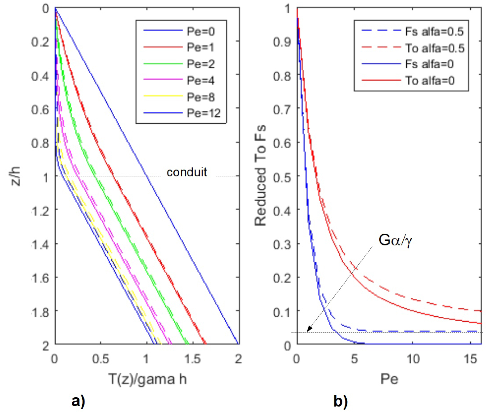
3.4. Case of a recharge window (Pe = Cst for 0 < x < L and Pe = 0 elsewhere)
General solutions of (23) are now investigated for the case of a recharge window (V ≠0) limited to the range x = 0 to L as illustrated by Figure 11a. Only the case 𝛽 = 0 is considered for sake of simplicity.
- for x < 0, V = 0 and the conduit is not recharged so that q(x) = 0; thus the standard conductive equilibrium T(x,z) =𝛾 z applies;
- for 0 < x < L, water infiltration with constant V occurs; it is supplying the conduit flow resulting in a flow rate increasing linearly according to q(x) = Vx;
- for x > L, V = 0; for x > L, q(x) is now constant and becomes q(x) = Vx.
For x < 0, the assumed initial conduit temperature is just Toini =𝛾 h.
Cross section along x direction showing the effect of a limited infiltration (0 < x < L = 20 h) recharging the conduit. (a) Represents the evolution of the water flux q(z) in the conduit and (b) plots the normalized conduit temperature T0(x) for several Pe values. The dotted lines show the numerical value and the full lines the approximation of (36) of Section 3.4.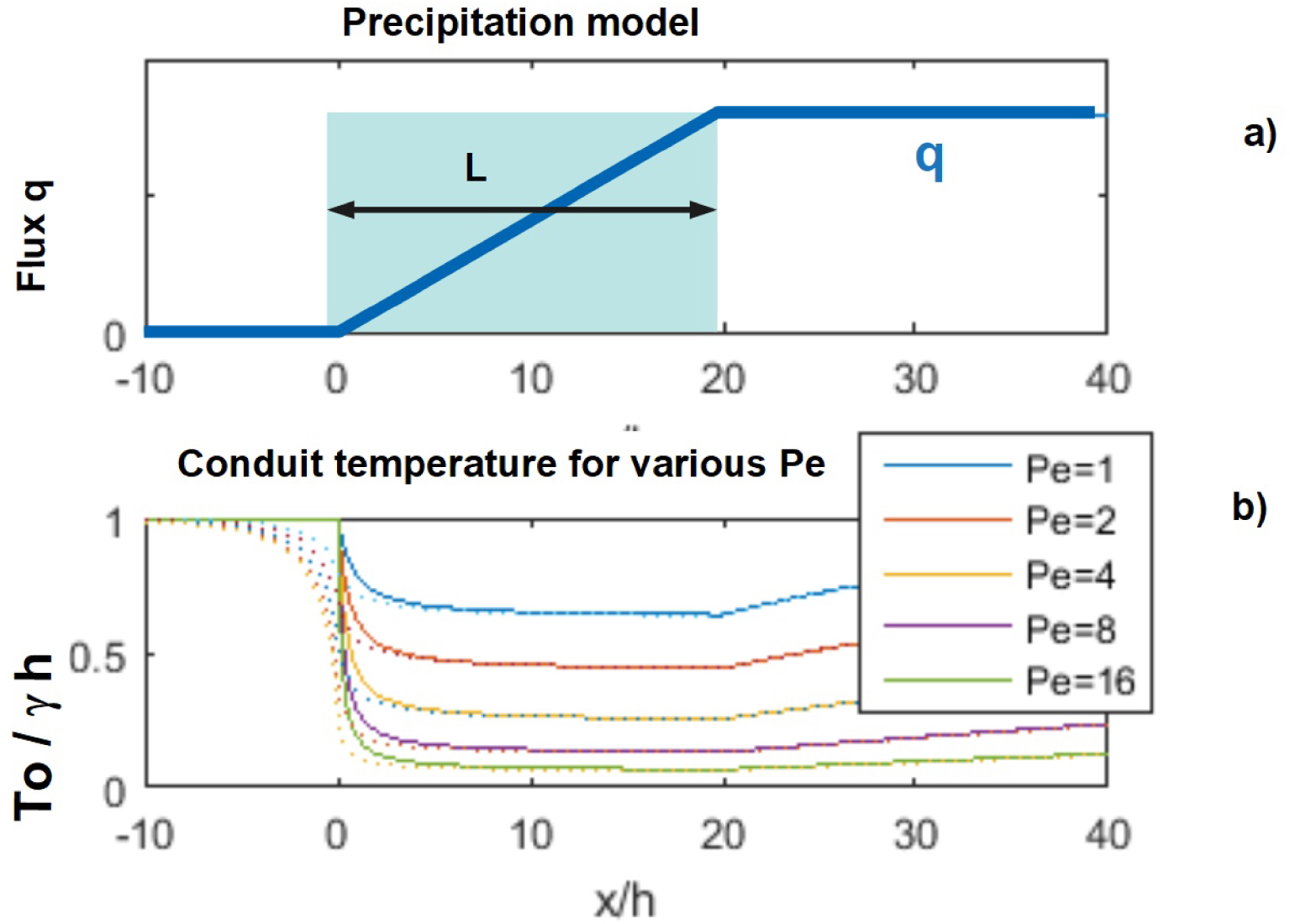
For 0 < x < L, T0(x) is solution of:
| (34) |
| (35) |
It is possible to avoid the singularity of the solution (35) at x = 0 by adding into (34) a dissipating term in the energy budget; this dissipating term accounts for horizontal conduction along x limited to a horizontal strip of half thickness h∕2 around the conduit. The boundary condition now applies: after a few development detailed in Appendix A, for large Pe, the solution of the modified equation is now:
| (36) |
When for z > L, the recharge is stopped; q(x) remains constant and equal to VL but the model has to be adapted. This is because, in this case, Equation (10) becomes simply ∂2 T+∕∂z2 = 0: the vertical temperature profile is simply linear above and below the conduit. But, at the level z = h, the slopes of these two linear segments are different in order to compensate for the horizontal decay of the convective heat flow in the conduit. The heat budget of the conduit writes:
| (37) |
| (38) |
| (39) |
The final result of this study is that, when infiltration supplying the conduit flow occurs abruptly in x, the established regime is rapidly dominant in x except in a narrow range of x values (on the order of ). Also when the supply is suppressed for x > L, T0 decreases exponentially with a characteristic length PeL so that this decrease in x is very slow. Furthermore the integral solution described above allows to generalize these results for varying Pe, Pe being replaced by its arithmetic average. Since in the actual case h≪L and Pe > 1, the practical conclusion is that the actual thermal data of T0 can be directly compared to the prevision of the model through (26)–(28). These analytical results can now be compared to actual thermal data.
4. Application of the model to Lez data; results and discussion
The available thermal data are: (1) the temperature of the Lez spring which is identified to T0 at the output of the system, (2) the near surface temperature gradients in shallow boreholes (Fs∕K) and (3) the deep temperature trend extrapolated onto the ground surface (Textrap) from oil exploration data extrapolation. Some parameters are well known constants such as (𝜌C) = 4.18 × 10⁶ W⋅°C−1⋅m−3, G = 0.23 °C/100 m; others apply to the site (cf Section 2) such as rock conductivity K = 2.75 W⋅m−1⋅°C−1, deep geothermal gradient 𝛾 = 3.1 °C/100, length of the system L = 15,000 m.
However the head gradients along the vertical path 𝛼 = −dH∕dz and along the horizontal paths 𝛽 = −dH∕dx also need to be defined; in the following, their value is speculated on the basis of available piezometric data. Water level has been continuously monitored in about 20 piezometers beginning in the 1980s [Avias 1995]. The observed difference of water levels between the upper part of the watershed and the spring is on the order of some tens of m and rarely exceeds 100 m [Karam 1989; Avias 1995]. This decrease of H along the water path is associated partly with the downward infiltration path (coefficient 𝛼) and partly with the horizontal path in the conduit (coefficient 𝛽); none of them is available from actual data. In order to appreciate the importance of the gravity-head potential term on the result, two extreme assumptions will be made:
- either 𝛼, 𝛽 are both 0 or at least very small i.e. a quasi hydraulic equilibrium occurs along the path; this implies no contribution to the energy transport since the gravity potential effect is fully compensated by that of the water pressure;
- or a head decrease on the order of 𝛿H = 100 m is occurring between the ground level and the spring; half of this decrease is assigned to the vertical path (𝛼 = 0.1 m/m for a vertical depth around 500 m as obtained below) and the other half to the horizontal one (𝛽 = 0.0067 m/m for a horizontal length around 15 km). The fact that 𝛼 >𝛽 reflects the fact that the impedance of the conduit is obviously much smaller than that of the porous medium.
4.1. Global parameters: use of T0 and Textrapol
The observations of T0 and Textrap are now used in the above 1D model to derive from (26)–(31) unknown parameters. These unknown quantities are h and Pe, but since Pe = (𝜌C)Vh∕K, it is clear the actual unknowns are h and V : in practice Pe may be expressed as Pe = 0.049Vh with h in m and V in m/year.
From the data T0 and Textrap,—eventually expressed as deviations, with respect to Tground—the value of h is easily computed using (31): the difference 𝛾h = Textrap − T0 gives h = 440 m. The average value of Pe is then obtained from (26). In the case 𝛼 =𝛽= 0 (26) reduces to 〈Pe〉 =𝛾 h∕T0 = 6. In the case 𝛼 = 0.1, 𝛽 = 0.01, Equation (26) leads to 〈Pe〉 = 6.8 which is significantly higher.
From these values of Pe, one can deduce the vertical specific discharge V = 0.28 m⋅y−1 in the first case (𝛼 = 𝛽 = 0) and V = 0.31 m⋅y−1 in the second one. These values of V are quite consistent with the estimate deduced from the water budget at the emergence: in order to supply the Lez spring, (2 m3⋅s−1 i.e. 63 × 106 m3⋅y−1), a precipitation area of 63∕0.28 = 225 km2 is required in the first case and 63∕0.315 = 200 km2 in the second one. This is smaller that the catchment area previously quoted (∼250 km2) but not in contradiction with various estimates of the area feeding the spring [Dausse 2015; Marechal et al. 2014].
4.2. Detailed interpretation of FS∕K data
According to (33) the apparent surface heat flow FS—the residual geothermal heat flow—is equal to the deep heat flow attenuated by a factor e−Pe plus a contribution of the gravity-head potential which tends toward KG𝛼 for Pe→ + ∞. The last contribution proportional to 𝛽 and related to the conduit flow is probably very small and therefore neglected; therefore Fs∕K should be larger that G𝛼 (i.e. 0.23𝛼 in °C/100 m). Actually some of the measured thermal gradients are very small and even reach 0. It cannot be excluded that some of these measurements are biased by vertical water circulation inside the well but most measurements seem sound. Since the value of 𝛼 may be vanishing for these wells, experimental T(z) profiles don’t provide any experimental proof for the occurrence of a positive lower bound for the temperature gradient which would indicate some significant positive value of G𝛼 for large Pe.
Previous studies have already proposed that gravity potential dissipation does affect the thermal gradient in underground water system [Manga and Kirchner 2004; Lismonde 2010]. In particular, Luetscher and Jeannin [2004] compiled observations of vertical temperature gradients in several thick karst systems; these gradients tend toward a small but positive value on the order of 0.3 °C/100 m (i.e. close to G) which could be associated with the dissipation of gravity potential. This result is clearly in contradiction with the present observations of thermal gradients but this also suggests that the temperature gradient was not estimated in the same conditions. According to the present model of saturated porous flow, a lower bound of thermal gradient near to G could occur only for very small fluid pressure (i.e. 𝛼 ∼ 1); therefore the occurrence of lower bound close to G would imply that, for such data, water is flowing at pressure conditions which remain close to the atmospheric pressure i.e. in unsaturated conditions at least during part of the flow circuit. Therefore differences in saturation conditions could explain the apparent paradox.
Anyway, the horizontal variations of present observed thermal gradients may be interpreted qualitatively in term of Pe according to Pe = −log(FS∕K) so that FS∕K reflects at least qualitatively the local value of the product Vh. According to measurements, a zone of very low gradient values and therefore of large Pe is observed on Figure 6. The wells with labels 3 Mas de Vedel (0.13 °C/100 m), 4 Bois de St Mathieu (0.5 °C/100 m), 6 les Matelles (0.13 °C/100 m), 7 Ferrieres (0 °C/100 m), 25 Frouzet (0.15 °C/100 m), 9 Claret (0.42 °C/100 m) have been drilled in Jurassic layers; all of them are located in recognized zones of water loss physically connected to the Lez spring as shown by dye tracing [Marechal et al. 2014]. This confirms that low thermal gradients areas correspond to high infiltration rate (i.e. high V ). Inversely, relatively high values of gradient ( > 2 °C/100 m) occur in the eastern and northern border of the catchment; this is consistent with the lack of connection with the spring as observed in these areas by dye tracing [Marechal et al. 2014]. Besides, the polynomial trend of Figure 7 suggests that the central zone of very low thermal gradient (high infiltration?) extends toward the West. This rapid comparison indicates the interest of high precision temperature measurements in shallow boreholes for mapping recharge zones.
4.3. Global evaluation of integrated energy fluxes
Due to the small number and values of measured surface gradients, it is impossible to define a single value characterizing the near surface heat flow. Nevertheless an integrated value is available through surface integration of the observed values of FS over the watershed area would reflect the integrated value of the residual geothermal flux—once part of it is absorbed for heating the water. Evaluation of Eresid = ∫FS requires the knowledge of FS on the whole area. As the distribution of the available data is uneven and quite sparse, the trend displayed on Figure 7 is used and the surface integral over the whole domain is computed. The resulting residual energy Eresid is 5.8 MW. In the interpolation of Figure 7 some negative values of FS have been obtained in the centre of the basin; when these values are forced to 0, the change in Eresid is very small (6.02 MW instead of 5.8). On Table 2 this integral is compared with other values of the energy associated with the system.
Evaluation of the various integrated energy fluxes
| Name | Explanation | Integrated energy (MW) | Corresponding area (km2) | Average energy flux (W⋅m−2) |
|---|---|---|---|---|
| Egeoth | Available geothermal flux over the catchment: ∫K𝛾dS | 21 | 250 | 0.085 |
| Eresid | Residual thermal flux over the catchment; ∫FSdS | 6 | 250 | 0.021 |
| Egeoth − Eresid | ∫K𝛾dS −∫FSdS | 15 | 250 | 0.064 |
| Egravity | Gravity head potential component PeKG(𝛼h +𝛽 L∕2) | 0 to 1.1 | 250 | |
| Espring | Output of the spring (𝜌C) Q𝛥T | 19 | - | - |
The difference between the geothermal flux of deep origin Egeoth and that observed at the surface Eresid is of the same order as the observed Espring but somewhat smaller by about 25%. It is therefore interesting to study whether the gravity head potential term could contribute significantly to the output temperature: according to the heat budget of the model (33), the component of gravity-head potential should be added as an extra energy to the difference Egeoth − Eresid. In the case of 𝛼 = 0.1 which is an upper bound, for Pe = 6.8 as suggested in Section 4.1, this component Egravity amounts to 1.08 MW which is significant but clearly too small to explain the gap between Espring and the captured geothermal heat flow Egeoth − Eresid. Many explanations for this gap may be suggested: they could proceed from errors in the energy budget such as the underestimate of Egeoth or the overestimate of Espring. However this gap could also derive from some inherent simplification of the model; two of them are briefly discussed below.
A first explanation could be that the geothermal heat flow is in fact captured over an area larger than the assumed 250 km2, as a result of 3D concentration: under this effect, the deep flow lines of the geothermal heat flow would naturally deviate from vertical and tend to converge toward the underground exchanger associated with deep water circulation. As suggested by Badino [2005], this three dimensional effect can be estimated using standard conductive models developed for the design of heat exchangers. Let assimilate the characteristics of the exchanger (the deep conduit) to a horizontal disk with radius R = 8 km (area ∼ 200 km2) located at depth h = 440 m (simplified geometry required to evaluate its “shape factor” Sf = 4πR∕acotg(R∕2h)) and submitted to a heat flow K𝛾 of deep origin. Assume for simplicity that the imposed temperature is 0 at the ground surface and 0 at the disk surface. The linearity of the heat equation allows to superimpose two fields of temperature: (1) the field associated with a disk with imposed temperature −𝛾 h and no heat flow at z = ∞ plus (2) the field due to a single gradient 𝛾z. The absorbed conductive heat flux transferred from the medium to the disk amounts to:
| (40) |
A second explanation implies possible transient effects due to external factors forcing such secular variations in water circulation. So far, the budget evaluation use the steady state assumption which rules out such possible environmental changes. The impact of sudden change such as the onset of water circulation can be studied using time dependent solutions of (10)–(15); the time dependent equations are written by replacing “ = 0” in (10)–(11) by “ = (𝜌C)r ∂T∕∂t” and their transient solutions are obtained analytically by Laplace transform followed by numerical inversion. Assume, for example that, starting from an initial conductive equilibrium (Pe = 0), the water flow is suddenly switched on with Pe = 6 at time t = 0. From this epoch up to now, the temperature field evolves toward a new equilibrium and the transient response of the temperature profile propagates downward according to two characteristic times: the diffusive time 𝜏diff = z2∕𝜅 = 3200 y (where 𝜅 is the rock diffusivity ∼2 × 10⁻⁶ m2⋅s−1) and the convective time 𝜏conv = z∕V ∼ 200 y (for V = 0.5 m⋅y−1). Instantaneous temperature profiles are shown in Figure 12a for various values of time following the onset of circulation; they illustrate how the upper layer is quite rapidly cooling whereas the temperature disturbance propagates downward slowly, in the conductive zone z > h. The evolution of the conduit temperature as a function of time is also illustrated by Figure 12b, showing that time for reaching the equilibrium temperature is in the order of 10,000 y; this emphasizes the delayed effect of very ancient modifications of the flow which could explain the apparent discrepancy derived from steady state assumptions (e.g. by overestimating the output temperature of the spring and its energy output, since steady state is not yet reached).
(a) Calculated profiles of T(z,t) resulting from the onset of water circulation (Pe = 6) starting at time 0 from a conductive profile. Initial condition (conductive equilibrium) and final one (steady state) are shown as well as several intermediate profiles at various times. The parameters have been adapted to the Lez case (Tground = 13.5 °C, 𝛾 = 3.1 °C/100 m, h = 440 m, Pe = 6). (b) Resulting temperature T0 at z = h evolving as a function of actual time in y.
5. Conclusion
Available geothermal data around the catchment of the Lez spring offer the opportunity of developing and of applying a geothermal model based on the principle of energy conservation. The energy source is mainly provided by the geothermal heat flux; this energy is exchanged with the fluid during its diffuse flow inside the karstic porous/fractured matrix connected to a conduit until the spring outlet where it is pouring. In order to assess quantitatively the nature and amount of energy captured by this natural heat exchanger, a simplified physical model is developed based on the universal laws of mass and energy conservation in steady state conditions. It leads to second order differential equations for the fluid temperature with boundary conditions which are specific of hydro-geothermal problems encountered in karstic areas. Owing to various simplifying assumptions (simple geometry of the exchanger, negligible horizontal heat conduction) the equations can be solved analytically; simple expressions for temperatures and heat fluxes are proposed as functions of Pe,h plus parameters associated with hydraulic gradients.
This model cannot pretend to account for the actual complexity of the karstic medium but it provides the parameters of a simplified system which is energetically equivalent to the actual flow. The offset observed between the actual ground temperature and the trend of the deep thermal data gives the depth h ∼ 440 m of the conduit. A mean Peclet number Pe ∼ 6 can be evaluated from the excess of the spring temperature with respect to that of the rain. An energy budget integrating the various energy fluxes—i.e. (1) deep geothermal flux, (2) residual surface flux deduced from shallow temperature profiles and (3) heat advected at the spring—is presented. The difference between the two first fluxes is insufficient to account for the third one so that a further component of energy is needed. The energy component associated with the dissipation of gravity potential is too small; other explanations are discussed such as 3D effects in the geothermal flux and the occurrence of transient effects due to environmental changes.
In this work, specific attention is directed to the various energy sources affecting fluids, the potential gravitational energy, in particular. Following Stauffer et al. [2014], the correct energy balance transports methalpy, which includes enthalpy (i.e. thermal energy plus fluid pressure) plus the potential energy of gravity, The other terms (kinetic energy and friction energy) are omitted as negligible for porous flow. In water saturated media, the conduction–advection equation for energy involves the transport of hydraulic head H which includes both pressure and gravity potentials; since the vertical fluid pressure gradient tends to compensate the effect of gravity, the contribution of H to the energy balance is much smaller than that of gravity potential alone (which would, on its own, result in a component of vertical thermal gradient up to G = 0.23 °C/km) but nevertheless significant. This concept is tentatively applied to the model (and data) of the Lez spring at two levels. Firstly, at the global level, the contribution of gravity-head term is evaluated and could amount to less than 5% of the total energy contribution. Secondly, at the level of single thermal profiles, the gravity and head contribution would eventually result in a lower bound for thermal gradient affected by downward flow; however, from actual thermal profiles obtained in the area, no such lower bound of thermal gradient was evidenced suggesting that the gravity head contribution is not so important.
Data presented here have been obtained in the 80s before recent active management of the Lez output; a systematic campaign of measurements would certainly permit actualization and specify the regional pattern of residual heat flow.
Further investigations and in particular, high precision thermal loggings are required to answer this question definitively, as well as the role of gravitational potential.
Conflicts of interest
The author has no conflict of interest to declare.
Acknowledgments
This work was initiated following discussions with Michel Bakalowicz, Francis Lucazeau, Véronique Leonardi and Hervé Jourde. The development of the mathematical model received assistance from Pierre Genthon. The possible importance of the gravitational potential was pointed out by Patrick Lachassagne and resulted in discussions with Patrick Goblet, Emmanuel Ledoux and Ghislain de Marsily. The author apologizes for committing a basic error in a previous version of the manuscript while omitting the influence of pressure in the energy budget.
Most of the data come from the collections of CERGA (Centre pour l’Enseignement et la Recherche en Geosciences et Applications) which has been recording and storing most of the hydrogeological studies on the Lez karstic system; the help of Josè Gravellec, Pierre Bérard, Jean Pierre Faillat and Jean Christophe Marechal is gratefully acknowledged.