Random fields and up scaling, towards a more predictive probabilistic quantitative hydrogeology

Benoît Noetinger

doi:10.5802/crgeos.188

Random fields and up scaling, towards a more predictive probabilistic quantitative hydrogeology

Benoît Noetinger ¹

¹ IFP Energies Nouvelles, France

Comptes Rendus. Géoscience, Volume 355 (2023) no. S1, pp. 559-572.

Abstracts

English
French

Random fields are becoming a mature tool sharing applications in many area of physics, mechanics and geosciences. In the latter, it is commonly used under the name of geostatistics. Continuous enrichment of geological/geostatistical models leads to manipulating hydrogeological models characterized by many parameters or hyperparameters corresponding to statistical aggregates that may be poorly estimated due to the scarcity of field data. Those parameters are generally support-scale-dependent and uncertain, so some inverse problem and uncertainty analysis must be carried out in practical applications that involve generally some forward calculation for example a fluid flow simulation if one in interested in transfers in the subsurface. Up scaling techniques are still required to find and to restrict in a controlled manner the more relevant parameters, allowing to lower the dimension of the parameter space. In the stochastic case, the interaction between the conductivity spatial distribution and the flow pattern can lead to non trivial behaviours that will be discussed. Fractured media will not be considered. That note does not present original results, but a selection of some potentially fruitful research avenues suggested by previous works.

Le raffinement continu des modèles géologiques/géostatistiques conduit à manipuler des modèles hydrogéologiques caractérisés par de nombreux paramètres dépendant en général de la position dans l’espace, voire des hyperparamètres correspondant à des agrégats statistiques sous-jacents. Du fait du manque de données, ils peuvent tous être mal estimés. Ces paramètres dépendent généralement de l’échelle du support d’acquisition de la mesure liée à l’instrumentation employée. Une remise en cohérence spatiale nécessitant une analyse inverse du problème et de l’incertitude doit être effectuée pour les applications. Des techniques de mise à l’échelle s’avèrent alors nécessaires pour restreindre de manière contrôlée l’espace des paramètres les plus pertinents, permettant de réduire la dimension de l’espace des paramètres, ouvrant ainsi la voie aux applications. Cette approche nécessite la quantification de l’information pertinente. Dans le cas stochastique, l’interaction entre la distribution spatiale de la conductivité et le modèle d’écoulement peut conduire à des comportements non triviaux qui seront discutés. Par souci de concision, le cas des milieux fracturés ne sera pas considéré. Ce court texte vise surtout à mettre en lumière quelques pistes de recherche prolongeant les résultats présentés.

Metadata

Received: 2022-04-11
Revised: 2022-11-04
Accepted: 2022-11-22
Online First: 2023-02-27
Published online: 2024-02-23

DOI: 10.5802/crgeos.188

Keywords: Applied geosciences, Porous media, Disorder, Upscaling, Geostatistics, Quenched disorder
Mot clés : Géosciences appliquées, Milieux poreux, Désordre, Mise à l’échelle, Géostatistique, Désordre gelé

Author's affiliations:

Benoît Noetinger ¹

¹ IFP Energies Nouvelles, France

License:

CC-BY 4.0

Copyrights: The authors retain unrestricted copyrights and publishing rights

@article{CRGEOS_2023__355_S1_559_0,
     author = {Beno{\^\i}t Noetinger},
     title = {Random fields and up scaling, towards a more predictive probabilistic quantitative hydrogeology},
     journal = {Comptes Rendus. G\'eoscience},
     pages = {559--572},
     publisher = {Acad\'emie des sciences, Paris},
     volume = {355},
     number = {S1},
     year = {2023},
     doi = {10.5802/crgeos.188},
     language = {en},
}

TY  - JOUR
AU  - Benoît Noetinger
TI  - Random fields and up scaling, towards a more predictive probabilistic quantitative hydrogeology
JO  - Comptes Rendus. Géoscience
PY  - 2023
SP  - 559
EP  - 572
VL  - 355
IS  - S1
PB  - Académie des sciences, Paris
DO  - 10.5802/crgeos.188
LA  - en
ID  - CRGEOS_2023__355_S1_559_0
ER  -

%0 Journal Article
%A Benoît Noetinger
%T Random fields and up scaling, towards a more predictive probabilistic quantitative hydrogeology
%J Comptes Rendus. Géoscience
%D 2023
%P 559-572
%V 355
%N S1
%I Académie des sciences, Paris
%R 10.5802/crgeos.188
%G en
%F CRGEOS_2023__355_S1_559_0

Benoît Noetinger. Random fields and up scaling, towards a more predictive probabilistic quantitative hydrogeology. Comptes Rendus. Géoscience, Volume 355 (2023) no. S1, pp. 559-572. doi : 10.5802/crgeos.188. https://comptes-rendus.academie-sciences.fr/geoscience/articles/10.5802/crgeos.188/

Version originale du texte intégral (Propose a translation )

1. Introduction

The use of numerical models for studying subsurface flow has become common practice in hydrology and petroleum engineering over the last 50 years [Renard and De Marsily 1997; De Marsily et al. 2005]. However, one of the major questions that still poses a problem is that the data needed to build an accurate model are incomplete in essence. Although contemporary computers are growing ever more powerful and capable of describing the relevant flows with increasing details, the required input data growth imposes a major increase in computing facilities if one wants to explore correctly the uncertain input parameter space in order to make the best decisions [Gorell et al. 2001]. In many applied geosciences issues, the basic concern is to recover, to store or to follow some fluid, waste or even thermal energy in subsurface formations at good economical conditions, while minimizing overall environmental risks. Most of the associated transport processes occur in the porosity of natural rocks, perhaps fractured, so studying flow in porous media at several scales is a major issue. In order to proceed, a concise macroscopic description of flow in porous media encompassing several scales without knowing the exact structure of the subsurface at lower resolution scales must be obtained.

Basically one wants to be able to estimate with some accuracy the average value, as well as the associated variance of any simulated value of interest. Knowledge of the full probability distribution is in general not required, although knowing if the resulting distribution is approximately Gaussian or not may be important. In the general case, when the driving equations relating input data to output observables are strongly non-linear, extensive Monte-Carlo sampling of the input parameter space is required to get estimations of these output statistical quantities. A typical subsurface model is generally described by some random fields of say porosity, permeability maps conditioned to several field observations, sedimentary layer shapes, aquifer positions, etc…These random maps depend in turn on some hyperparameters of statistical nature such as variance, drift, correlation scale: that is the aim of geostatistics that will be presented with more details in Section 2.1. In addition, some man-controlled parameters such as the position of wells and the associated flow rates enter as input data in the model. For applications, that influence of that set of parameters may be sampled by simulation to select the best position and management of the wells.

Using such models, we are led to consider high dimensional parameter spaces, both for the random set of natural data, and for the man-controlled parameters. Consider a parameter space of N = 100 dimensions, and by hypothesis, let us assume that each parameter can take only 2 values. An exhaustive exploration of that parameter space will imply being able to perform 2¹⁰⁰ independent runs, that is clearly impossible even with hypothetical quantum computers. In addition, in current models, most parameters belong to some continuous interval, increasing the effective dimensions of the parameter space. So following any exhaustive approach is a dead end. Many alternative sampling techniques were developed [Zhang 2001]. Experimental design techniques coupled with machine learning methods are being developed [Scheidt et al. 2007; Santos Oliveira et al. 2021, and references therein].

That implies that some systematic workflow is to be built in order to reduce the number of dimensions of the effective working space under consideration. As that situation presents some similarities with statistical physics, some bridges between both disciplines can be expected: a description of these connections may be found in Noetinger [2020]. To sum-up, similar issues are at the heart of one the most active area of complex systems understanding, the so-called spin glasses for which G Parisi was awarded the 2021 Nobel prize in physics [Mézard et al. 1987; Zdeborová and Krząkała 2007; Zdeborová and Krzakala 2016]. In the geoscience side, some reviews illustrate similar issues [Gorell et al. 2001; Floris et al. 2001; De Marsily et al. 2005].

The goal of that short paper is to suggest some avenues of research in order to provide answers to the following questions:

What is the amount of information that is required to build a useful numerical model with a degree of sophistication consistent with the input knowledge.
is it possible to build a model that may be continuously improved as our knowledge of the particular aquifer increases along with the volume of data acquisition.

The paper is organised as follows: in Section 2, we provide some general elements. Then a focus is given in Section 2.1 about geostatistics, before giving some elements about information quantification in Section 2.2. Single phase flow problem serving as a basis for most of our discussion is introduced in Section 2.3. Then we discuss up-scaling applications in Section 3.1 by discussing the scale and support effects. Non linear issues implying a strong feed-back between the medium structure and the flow are discussed in the case of two-phase flows in Section 3.2. In Section 4, we present some ideas allowing to merge the preceding considerations between geostatistics, up-scaling and information theory for practical applications. Finally some fruitful research avenues are suggested for future investigations.

2. Medium description, up-scaling issues

We consider a subsurface formation of typical kilometric scales. In Figure 1, the overall scales of the considered aquifer are represented, as well as the corresponding discretization mesh of interest, choosen cartesian for sake of simplicity. Each grid block may be populated by parameters such as porosity 𝛷(r), permeability k(r) and any other relevant parameter. That can be drawn using some deterministic or geostastistical software.

Figure 1.
Geometry of the problem on a simplified 2D section of a subsurface model domain 𝜔. A coarse grid made of blocks 𝛺 of typical size L is super-imposed to a geological fine grid of typical size 𝛥 in order to solve the conservation equations of interest. The intermediate scale 𝜆 serves in posterior treatments for checking the overall consistency of the model. Reprinted (adapted) from Colecchio et al. [2020] Copyright 2020 with permission of Elsevier.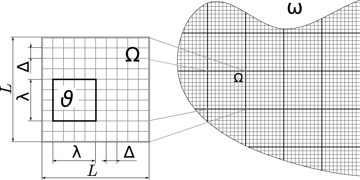

2.1. About geostatistics

Modelling subsurface formation using numerical models implies to account for the fact that any local quantity of interest may depend on position vector r. In most cases, for example the quenched¹ positive permeability k(r), is represented as being a random function of position. It is characterized by some mean-value and fluctuations that are measured using field data (an issue in itself!). That is the aim of the so-called geostatistical approach, originaly founded by Matheron [1963], Krige [1976], De Marsily et al. [2005], Chiles and Delfiner [2009] and developed by several others, that form the conceptual basis of several popular commercial softwares. The basic idea is to interpolate known measurements on a given support on several locations by inferring some underlying statistical structure. Notice that the primary random mathematical objects are functions or fields that are characterized by an infinite number of degrees of freedom. So the most natural embedding formalism that encompasses it is the so called field-theory employed in both statistical mechanics or particle physics [Noetinger 2020; Hristopulos 2020]. Another related issue that was pointed-out by Tarantola [2005] is that working with continuous variables implies that there is not a reference entropy measure allowing to quantify easily the information of a geostatistical distribution: the overall results are sensitive to the coordinate system used by the modeller. At this stage, the associated reference “non-informative” reference distribution [Tarantola 2005; Abellan and Noetinger 2010] is not determined. That explains some deep theoretical and practical difficulties for generalizing the approach to curved spaces or to non-uniform grid, Mourlanette et al. [2020]: such a situation may occur if tectonics imply strong deformation of a sedimentary basin. In most practical cases, some implicit cartesian assumption is made. Probably it could be justified using the sedimentary nature of most aquifers. In the similar statistical physics case, it may be shown that the continuous Boltzmann–Gibbs distribution that is the basis of most applications may be derived by a suitable limit of the underlying quantum mechanics processes that poses paradoxically less difficulty owing to their discrete nature (Setting-up a natural probability measure to a 6 face dice rather than to a continuous process). In geoscience, approximate Log-normal distributions (the logarithm of the conductivity is a Gaussian distributed variable) were observed at the core scale within several geological environments [Gelhar 1993]. Note that in most cases, the amount of data is not sufficient to provide the form of the probability distribution function (pdf) of k, and higher order correlation functions are almost impossible to be determined from field data. In the current modelling practice, they are implicitly fixed by choosing some additional assumptions based on geological expertise on similar environments. As a consequence, even the input stochastic model is questionable.

Another class of models that intend to add information on high order correlation functions are multipoint or so-called process-based models, intending to reconstruct the apparent randomness of the subsurface by simulating the long term history of the formation using some dynamical physically based model: Diggle et al. [1998], Granjeon and Joseph [1999], Hu and Chugunova [2008], Michael et al. [2010]. These models introduce more physically based parameters and are more realistic. However, they may depend on assumptions regarding the time-dependant external forcing at their boundaries, introducing stochasticity in a somewhat another manner. An essential specificity of geosciences is the so-called measurement support effect: any data is obtained using some instrumentation that averages the details of the process at hand on a characteristic length that depends on the physical process. That scale may vary from some centimeters for laboratory/logging tools, to hectometers in geophysics corresponding to the typical wavelength of geophysical waves, or to the support of transient well tests interpretation. Any measurement is characterized by a support scale characterizing the measurement itself, and by another spatial scale that is the typical resolution.

Finally, due to the data scarcity, it is necessary to up-date any prior model of the subsurface by accounting for the additional data that are continuously enriching the available information. That new data can be provided by pressure and rates measurements at some producing wells, time-dependant tracer concentration showing connections between several regions of the subsurface etc…This is the so called inverse problem issue that was addressed by many authors [Jacquard 1965; LaVenue et al. 1995]. It is well-known that such problems are ill conditioned and that some regularization is required [Tarantola 2005; Oliver and Chen 2011, and references therein]. That can be achieved accounting for a prior geostatistical structure [LaVenue et al. 1995; Le Ravalec et al. 2000; Hu and Chugunova 2008] that is easier to carry-out considering gaussian priors.

2.2. Quantification of information

As data may be scarce (but even redundant), it is essential to be able to quantify the amount of information provided by a measurement, as well as the quantity of information that is required to make faithful predictions. That idea can be formalized using information theory, as attempted in Abellan and Noetinger [2010, and references therein]. A quantitative estimate can be defined introducing the relative entropy (Kullback–Leibler divergence) between posterior and prior distribution that serves as a non-informative reference distribution. That quantity is defined by:

I (p) = I (p | 𝜇) = \int p (m) log \frac{p (m)}{𝜇 (m)} d m .

(1)

Here, p(m) is the posterior distribution of m given that some measurement was carried out on the system. 𝜇(m) denotes the prior distribution m. For clarity, it is easier to introduce some discretization of m on a regular grid. So m is represented as a realization of the M dimensional vector, so m = (m(x₁),…,m(x_M))^t. The corresponding 𝜇(m) is assumed to be centered and multigaussian so the corresponding probability measure is given by 𝜇(m) ∼exp−1∕2(m ⋅C_p ⋅m) with a gaussian covariance matrix with elements that are given by:

C_{p} (x_{i}, x_{j}) = 𝜎_{0}^{2} exp (\frac{- | x_{i} - x_{j} |^{2}}{ℓ_{c}^{2}})

(2)

with

ℓ_{c}^{2}

is the correlation length, and

𝜎_{0}^{2}

the associated variance. Then the relative entropy I_MN of a posterior distribution corresponding to N linear measurements with independant errors

𝜎_{d}^{2}

gathered as a N dimensional vector F ⋅ x is given by I_MN:

I_{M N} = \frac{1}{2} log | I_{N} + C_{𝜈}^{- 1} \cdot F^{t} C_{p} F |

(3)

where |⋯| is the determinant of the square matrix ⋯ . Considering the specific problem of local measurements of the random field m at N different locations (x₁,…,x_N),N < M with measurement errors

𝜎_{d}^{2}

, one is led to evaluate:

\begin{matrix} I_{M N} (x_{1}, \dots, x_{N}) \\ = \frac{1}{2} log |{(𝛿_{i j} + \frac{𝜎_{0}^{2}}{𝜎_{d}^{2}} exp \frac{- | x_{i} - x_{j} |^{2}}{ℓ_{c}^{2}})}_{1 ⩽ i, j ⩽ N}|, \end{matrix}

(4)

when the measurement locations are far apart (typically all distances greater than ℓ_c), one gets the estimation:

I_{M N} (x_{1}, \dots, x_{N}) = \frac{N}{2} log (1 + 𝜇^{2}) with 𝜇^{2} = \frac{𝜎_{0}^{2}}{𝜎_{d}^{2}} .

(5)

Figure 2 illustrates present results that were also generalised to pumping test analysis and non-linear flow driven issues in Abellan and Noetinger [2010].

Figure 2.
Left: A typical realization of a random map 2D section of a subsurface model on a domain 𝛺, representing Log(k). The superimposed circles correspond to N = 5 physical measurements of permeability on a support scale with the corresponding radius, with several realistic values. The average distance between the circles corresponds to the coverage of the area. In a perfect situation, all the area should be covered, that is seldom the case. Right: the amount of information provided by N local measurements defined by the relative entropy of posterior distribution versus prior. Note the saturation of the information once the medium is well covered by the measurements, 𝜇 is defined in the main text. L^x and L^y are the overall size of the domain in the x and y directions, $ℓ_{0}^{x}$ and $ℓ_{0}^{y}$ denote the correlation length in corresponding directions. N^∗ is thus the number of correlated volumes inside the overall domain. It corresponds to the crossover the transition of information content between independent measurements and redundant ones. Copyright 2020 with permission of Springer-Nature.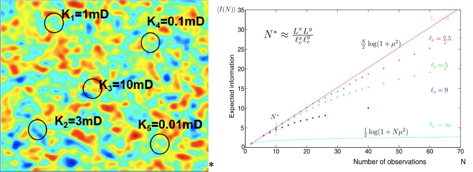

2.3. Fluid-flow modelling

In most cases, modelling fluid flow in a porous formation [De Marsily 1986] leads to solve a diffusion-like equation that reads:

𝜙 c_{t} \frac{\partial p (r, t)}{\partial t} = 𝛻 \cdot (k (r) 𝛻 p (r, t)) + f (r) .

(6)

Here, the parameters p(r,t), c_t and f(r) are respectively the time-dependent potential of interest, the total compressibility, and a source term. Dirichlet or Neumann Boundary conditions are known at the boundary of the domain 𝜔. Once that potential is known, associated transport problems can be solved, including multiphase flow issues that are not in the scope of present paper.

The basic issue is to be able to solve such equations, accounting for both the the effect of heterogeneities, and to be able to quantify the related uncertainties. In that context, analytical methods were developed by hydrogeologists [Gelhar 1993; Dagan 1989; Indelman and Abramovich 1994; Abramovich and Indelman 1995; Renard and De Marsily 1997], mathematicians [Jikov et al. 2012; Armstrong et al. 2019] and physicists, among other [King 1989; Noetinger 1994; Hristopulos and Christakos 1999; Nœtinger 2000; Attinger 2003; Eberhard et al. 2004; Teodorovich 2002; Stepanyants and Teodorovich 2003].

On the numerical side, a possible strategy is to transfer the small scale spatial fluctuations to a large scale support that encompasses the low spatial frequency components of the fields of interest. The calculations are carried out in practice using some numerical model in which the Laplace equation is solved using a grid of resolution L generally considerably much coarser than the input fine geological grid 𝛥 (notations in Figure 1), because the available computing power leads also to continuous improvement of local geological 3D representations. This implies obtaining a coarse grained Laplace equation with a renormalized conductivity map accounting as best as possible to the local subgrid variations. In the case of multimodal distributions, in which connectivity aspects are dominant, specific methods can be developed within the framework of percolation theory, such as real-space renormalization techniques [Berkowitz and Balberg 1993; Hunt et al. 2014; Hristopulos 2020].

In the stochastic context, a strategy is to average the solution of Equation (6) to get the average head (or pressure) ⟨p(r,t)⟩ in which the ensemble-average ⟨⋯ ⟩ is to be taken on the disorder of the conductivity field k(r) corresponding to a Monte-Carlo average over the disorder of the medium. Then, one can look for the equation that may drive that average head² [Noetinger and Gautier 1998].

3. About flow up-scaling

3.1. Single phase steady state up-scaling

It can be shown that under quite general hypothesis (statistical stationarity and convergence conditions) that the low frequency components of the average potential ⟨p(r,t)⟩ is driven by an effective equation that reads:

⟨ 𝜙 ⟩ c_{t} \frac{\partial ⟨ p (r, t) ⟩}{\partial t} = 𝛻 \cdot (K_{equ} 𝛻 ⟨ p (r, t) ⟩) + f (r) .

(7)

Here, the average ⟨⋯ ⟩ corresponds to an averaging over the randomness of the medium. The parameter K_equ is called the equivalent conductivity. It corresponds to the “natural” large scale relation between the mean flux and the large scale pressure gradient that can be provided by homogenization theories solving the so-called “auxiliary problem” to be solved numerically in x, y and z directions [Armstrong et al. 2019, and references therein], as it is illustrated Figure 3.³ Many expressions were proposed to relate K_eff to the underlying disorder [Renard and De Marsily 1997]. For one dimension, an elementary analytical calculation provides the harmonic average K_eff = ⟨k⁻¹⟩⁻¹. Generalizations of such a simple formula were proposed by many authors [Landau and Lifshitz 1960; Matheron 1967; King 1987, 1989; Dagan 1993; Neuman and Orr 1993; Noetinger 1994; Indelman and Abramovich 1994; De Wit 1995; Teodorovich 2002; Stepanyants and Teodorovich 2003; Colecchio et al. 2020; Nœtinger 2000]. Looking at the evolution of the permeability distribution, in 2 dimensions, numerically the log normal distribution appears to be stable under the up-scaling transformation, Figure 4 from Colecchio et al. [2020], analogous to the central limit theorem. That may be related to the duality argument of Matheron [1967] that justifies the geometric mean in 2D. In the 3D case, studying the emergence of a “stable” conductivity distribution invariant on the up scaling transformation would also be useful for studying strongly correlated systems having conductivity correlations decaying as a power law with the lag distance. This may be illustrated on Figure 4 below: in the practical side, in most cases, at present times, using a numerical technique is sufficient. In case of extremely heterogeneous media (that can correspond to bimodal media) at percolation threshold, a percolation transition may occur [Charlaix et al. 1987; Berkowitz and Balberg 1993; Hunt et al. 2014; Stauffer and Aharony 2014; Colecchio et al. 2020]. Its main consequence, a stabilization of the effective conductivity over a very large scale can be observed on Figure 5. In both situations, it appears that at some scale (becoming infinite just at the percolation threshold for an infinite small-scale conductivity contrast), the formation can be treated as an almost continuous medium: that is the so called self-averaging property that manifests itself once the characteristic size of the flow is larger than the typical correlation scale. Long ranged media, as well as media close to a percolation threshold remain a notable exception. The results presented in Figures 4 and 5 were obtained using a suitable post treatment of a single phase flow simulation on a large domain, without adding any external expansive Monte Carlo loop: that is sufficient to capture the dominant characteristic scales of the flow. In addition, in Figure 5, middle, it is illustrated the emergence of the so-called localization phenomena that is a consequence of high permeability contrasts [Arnold et al. 2019] that localizes high velocity regions in tiny regions, even in non-fractured media. Such flow-based maps are well suited for post-treatment: helping to build a coarse mesh, estimating critical paths that may control the overall uncertainties.

Figure 3.
Up-scaling geometry. The coarse block of size L have a detailed conductivity map given by geology. It is up-scaled by solving a steady-state quasi Laplace equation to determine an effective conductivity in the mean flow direction. Boundary conditions are usually no-flux parallel to the imposed mean flow, or periodic.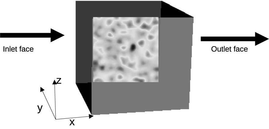

Figure 4.
Monte Carlo study of the dependance of the effective conductivity pdf with coarsening scale 𝜆. The overall flow is solved using several realizations of the input log conductivity map (left). The associated local dissipation map (center) allows to evaluate a distribution of coarsened effective conductivities averaged at intermediate scale 𝜆 [Colecchio et al. 2020]. The associated pdf’s are plotted (right). The self averaging feature is highlighted by the sharply peaked distribution around the geometric average for 𝜆 = 128 units. Reprinted (adapted) from Colecchio et al. [2020] Copyright 2020 with permission of Elsevier.

Figure 5.
Monte Carlo study of the effective conductivity pdf with coarsening scale 𝜆. The overall flow is solved using several realizations of the input bimodal map with conductivity contrast of 10⁴. The associated local dissipation map (center) highlights the localization phenomenon and allows to evaluate pdf’s of coarsened effective conductivities averaged at scale 𝜆 [Colecchio et al. 2020]. The resulting scale-dependant pdf’s are plotted (right). As the scale is increasing, the two peaks merge, the bimodal distribution disappears and becomes close to a log-normal distribution. The convergence to this asymptotic distribution shows critical slowing-down when the facies proportions are close to percolation threshold. In the infinite contrast case, scaling-laws are recovered [Stauffer and Aharony 2014]. Reprinted (adapted) from Colecchio et al. [2020] Copyright 2020 with permission of Elsevier.

3.2. About the interaction between the conductivity spatial distribution and the flow pattern

In several situations, such as when considering multiphase flow flows in heterogeneous media, some strong coupling between the flow and the underlying medium may occur. This can be the case when considering water displacing oil, CO₂ injection etc…This may give rise to an instability driven by a mechanism is similar to the well-known Saffman–Taylor instability that leads to viscous fingering if the displacing fluid is more mobile than the fluid initially in place. This emergence problem was studied by many authors such as Saffman and Taylor [1958], Homsy [1987], Tabeling et al. [1988], Tang [1985], Shraiman [1986]. A generalization to imicsible two phase flows was carried-out in the paper of King and Dunayevsky [1989, and references therein]. In that case, it appears a well defined sharp front separating both phases moves at the local velocity of the fluid, as shown in Figure 6, top. That front may be in unstable, by the same mechanism than the Saffman–Taylor instability, as shown in Figure 6, bottom. In the unstable case, an amplification of the heterogeneity effect is expected, while some smoothing arises in the stable case. The intuition suggests that a highly mobile

fluid will follow high velocity paths, its presence amplifying thus that advantage by a positive feed-back loop. This is the so called channeling issue. This problem was addressed by De Wit and Homsy [1997a, b], and revisited in the stochastic context by Artus et al. [2004], Nœtinger et al. [2004], Artus and Noetinger [2004], merging perturbation theory within the framework developed by King and Dunayevsky [1989]. In order to be more specific, the underlying equations reads:

\begin{matrix} 𝛻 \cdot [𝜆 (S (r, t)) k (r) 𝛻 p (r, t)] = 0 \end{matrix}

(8)

\begin{matrix} 𝜙 \frac{\partial S (r, t)}{\partial t} + 𝛻 \cdot (f (S (r, t)) U (r, t)) = 0 \end{matrix}

(9)

\begin{matrix} U (r, t) = - 𝜆 (S (r, t)) k (r) 𝛻 p (r, t) . \end{matrix}

(10)

Here, S(r,t), 𝜆(S(r,t)) and f(S(r,t)),S denote respectively the water saturation (local % of water, total mobility and the so-called fractional flow of water). This set of coupled equations may be solved numerically (it is at the heart of any multiphase flow in porous media simulator, to which additional complexities such as phase transitions and boundary condition management must be added). The saturation equation (9) is hyperbolic, leading to the formation of a shock front, whose stability is controlled by the jump of the total mobility 𝜆(S(r,t)) at the front.

Figure 6.
Dynamics of a two phase flow front moving in a heterogeneous rock, imposed mean flow from left to right, underlying random log normally distributed conductivity map top (a) stable case (b) Y averaged saturation at different times, bottom (c) fingering in the unstable case, (d) associated Y-averaged saturation at different times.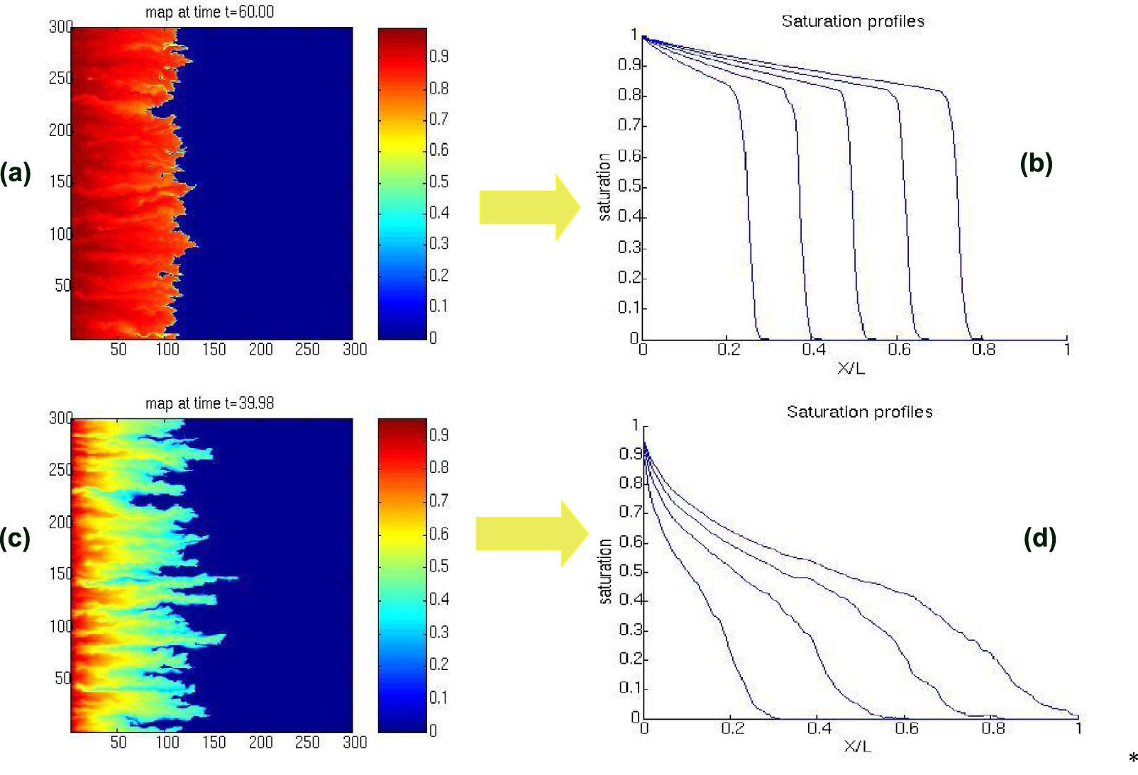

The technical difficulty for setting-up a perturbation expansion comes from the presence of the front that implies a mobility jump that renders perturbation theory a bit tricky [King and Dunayevsky 1989; Nœtinger et al. 2004]. The difficulty may be avoided by a suitable change of variable, using a working variable x(S,y,t) rather than S(x,y,t). It is thus possible to introduce the function x(S_f,t), in which S_f is the saturation of water just behind the front M_f is the corresponding total mobility jump M_f =𝜆 (S_f)∕𝜆(S = 0). The randomness of the underlying conductivity field propagates to the randomness of x(S_f,t), of average value ⟨U⟩t. At long times, the associated two point correlation function can be shown to converge to a well defined function in the stable case, while in unstable case it diverges, a manifestation of the spreading of the front [Tallakstad et al. 2009; Toussaint et al. 2012]. A possible approach of practical interest close to the single phase flow approach would be to look at an effective equation driving the ensemble-averaged water saturation ⟨S(r,t)⟩, or the Y-averaged saturation S(x,t). A diffusive-like regime arises in the case M_f = 1, that corresponds to a marginal stability criterion. In the general case, several proposals were reported long ago for characterizing the emerging large scale transport equation [Koval 1963; Todd et al. 1972; Yortsos 1995; Blunt and Christie 1993; Sorbie et al. 1995]. In the unstable case, one can consider that long fingers parallel to the imposed flow may be treated as a stratified medium. This leads to modify the fractional flow function with an ad-hoc change [Koval 1963]. In the stable case, it can be shown that the competition between the disorder that distorts the front and the viscous forces that tends to sharpen the front [Nœtinger et al. 2004] must lead to another form of the effective fractional flow, including some macrodispersion representing the net effect of the averaged disorder. In the infinite contrast case (e.g. immiscible gas injection) Diffusion Limited Aggregation (DLA) models were proposed, leading to a very rich literature involving percolation invasion models, fractals [Witten and Sander 1981; Wilkinson and Willemsen 1983; Paterson 1984; Masek and Turcotte 1993] with many contributions of SP.

4. Geostatistics, up-scaling and inverse modelling

Our original issue was to know the relevance of a complex model in regard to the input knowledge. It appears that if one is interested by predicting the average and variance of the output of some transport process, a compromise must be found between the overall accuracy of the calculation involving a high resolution grid implying large computing costs, and the statistical accuracy that requires being able to perform a huge number of Monte-Carlo simulations⁴ required to get representative statistical averages of the process under consideration. The overall simulation budget B(Size_model,N_MC) in terms of hours of CPU depends on the model size Size_model and the number of Monte Carlo simulations N_MC. The latter depends on the number of relevant input parameters that control the overall behaviour of the system. It is possible to determine the couple (Size_model,N_MC) such that the variance 𝜎²(Size_model,N_MC) of the prediction errors of the simulation output is minimized under the constraint of fixed B(Size_model,N_MC). As presented in the preceding section, up-scaling techniques may provide some tools allowing to get a case-dependent prior estimate of that variance without running the whole set of simulations.

Practitioners want to get estimations of the average value and of the variance of the output of interest (water supply, heat recovery etc…). So the approach developed by Abellan and Noetinger [2010] could be carried-out in the prediction space. The advantage of such an approach will be to be closer to operational quantities of practical interest, and also to be more independent on the dimension of the input parameter space. Such an avenue needs to be developed.

5. Conclusions and some perspectives

In that short note, we discussed some ideas and previous findings illustrating mainly the interaction of the quenched disorder of the natural media present at all scales to the flow. It appears that hydrologists could be greatly helped by developing an approach combining pragmatic practice, advanced averaging techniques and optimization techniques merged within a framework of physically guided artificial intelligence techniques. An approach is to draw the “phase diagram” of the problem at hand, i.e. the set of dominant parameters controlling the overall behaviour of the system, and providing descriptions of the critical behaviour of the system between the different regions of the phase diagram. Information theory concepts can be helpful to quantify the disorder and the amount of information of the system, providing useful links to statistical physics concepts and methods.

Such an approach is evidently process-dependant and must be adapted for heat or tracer transport and mixing, as well as reactive flows, issues that were not discussed in that short paper.

A promising approach would be to map the linear systems to be solved that are essentially of Laplacian nature into random matrix theory close to random graphs theory [Mohar 1997; Bordenave and Lelarge 2010; Potters and Bouchaud 2019]. That area of research is a fast growing field with applications for modelling networks such as the Internet, urban and road traffic, smart electrical networks, brain modelling, finance etc…Some applications may be found in the modelling of flow in fractured rocks [Hyman et al. 2017, 2019]. A possible mathematical approach is to study the spectrum of the large matrices obtained for solving the quasi Darcy flow equation that depends randomly on the geological input parameters. That may provide information about the effective number of relevant degrees of freedom that must be retained to describe the system [Biroli et al. 2007]. Depending on the degree of disorder, some eigenvalues of the associated Laplacian matrix can be expected to provide information while other eigenvalues may follow some universal distribution such as a Marchenko–Pastur distribution [Marchenko and Pastur 1967]. Such topics are deeply connected to classification methods by neural nets [Louart et al. 2018; Dall’Amico et al. 2019].

Finally, as illustrated by De Marsily [2009], water supply issues will become more and more critical, implying great applied and academic research efforts. As it was explained in present paper, expecting tremendous computing power cannot be the single option. The community will have to rely on innovative approaches at the cutting edge of modern science, as our mentors did [Matheron and De Marsily 1980; De Marsily et al. 2005].

Conflicts of interest

The author has no conflict of interest to declare.

Acknowledgements

The author is indebted to MM Alexandre Abellan, Alejandro Boschan, Ivan Colecchio Pauline Mourlanette and Alejandro Otero for their useful contributions.

¹ The term quenched is employed in statistical physics of disordered systems, it corresponds to systems having a fixed but unknown disorder without thermal fluctuations that reorganise it, a glass or an amorphous solid are typical quenched material.

² At first sight, averaging the driving equation looks to be simpler, and would evidently provide the arithmetic average for the conductivity, a clearly wrong result.

³ Notice that in the current practice, the result of the evaluation of these formula, or of the numerical solution of the auxiliary problem is used to populate the coarse grid of 𝛺 blocks, using the underlying local fine grid data. So the equivalent K_equ may still depend on position rather than the so-called K_eff that is intrinsic, it would correspond to working with an infinite volume 𝛺.

⁴ We implicitly consider that fully analytically solvable problems are very scarce!

References

[Abellan and Noetinger, 2010] A. Abellan; B. Noetinger Optimizing subsurface field data acquisition using information theory, Math. Geosci., Volume 42 (2010) no. 6, pp. 603-630 | DOI | MR

[Abramovich and Indelman, 1995] B. Abramovich; P. Indelman Effective permittivity of log-normal isotropic random media, J. Phys. A: Math. Gen., Volume 28 (1995) no. 3, pp. 693-700 | DOI | Zbl

[Armstrong et al., 2019] S. Armstrong; T. Kuusi; J.-C. Mourrat Quantitative Stochastic Homogenization and Large-scale Regularity, 352, Springer, Berlin, 2019 | DOI

[Arnold et al., 2019] D. N. Arnold; G. David; M. Filoche; D. Jerison; S. Mayboroda Localization of eigenfunctions via an effective potential, Commun. Partial Differ. Equ., Volume 44 (2019) no. 11, pp. 1186-1216 | DOI | MR | Zbl

[Artus and Noetinger, 2004] V. Artus; B. Noetinger Up-scaling two-phase flow in heterogeneous reservoirs: current trends, Oil Gas Sci. Technol., Volume 59 (2004) no. 2, pp. 185-195 | DOI

[Artus et al., 2004] V. Artus; B. Nœtinger; L. Ricard Dynamics of the water–oil front for two-phase, immiscible flow in heterogeneous porous media. 1–stratified media, Transp. Porous Media, Volume 56 (2004) no. 3, pp. 283-303 | DOI | MR

[Attinger, 2003] S. Attinger Generalized coarse graining procedures for flow in porous media, Comput. Geosci., Volume 7 (2003) no. 4, pp. 253-273 | DOI | MR | Zbl

[Berkowitz and Balberg, 1993] B. Berkowitz; I. Balberg Percolation theory and its application to groundwater hydrology, Water Resour. Res., Volume 29 (1993) no. 4, pp. 775-794 | DOI

[Biroli et al., 2007] G. Biroli; J.-P. Bouchaud; M. Potters Extreme value problems in random matrix theory and other disordered systems, J. Stat. Mech., Volume 2007 (2007) no. 07, P07019 | DOI | Zbl

[Blunt and Christie, 1993] M. Blunt; M. Christie How to predict viscous fingering in three component flow, Transp. Porous Media, Volume 12 (1993) no. 3, pp. 207-236 | DOI

[Bordenave and Lelarge, 2010] C. Bordenave; M. Lelarge Resolvent of large random graphs, Random Struct. Algorithms, Volume 37 (2010) no. 3, pp. 332-352 | DOI | MR | Zbl

[Charlaix et al., 1987] E. Charlaix; E. Guyon; S. Roux Permeability of a random array of fractures of widely varying apertures, Transp. Porous Media, Volume 2 (1987) no. 1, pp. 31-43 | DOI

[Chiles and Delfiner, 2009] J.-P. Chiles; P. Delfiner Geostatistics: Modeling Spatial Uncertainty, 497, John Wiley & Sons, New-York, 2009

[Colecchio et al., 2020] I. Colecchio; A. Boschan; A. D. Otero; B. Noetinger On the multiscale characterization of effective hydraulic conductivity in random heterogeneous media: a historical survey and some new perspectives, Adv. Water Resour., Volume 140 (2020), 103594 | DOI

[Dagan, 1989] G. Dagan Flow and Transport in Porous Formations, Springer-Verlag GmbH & Co. KG, Berlin, 1989 | DOI

[Dagan, 1993] G. Dagan Higher-order correction of effective permeability of heterogeneous isotropic formations of lognormal conductivity distribution, Transp. Porous Media, Volume 12 (1993) no. 3, pp. 279-290 | DOI

[Dall’Amico et al., 2019] L. Dall’Amico; R. Couillet; N. Tremblay Classification spectrale par la laplacienne déformée dans des graphes réalistes, GRETSI 2019 - XXVIIème Colloque francophone de traitement du signal et des images, August 2019, Lille, France (2019) (ffhal-02153901)

[De Marsily et al., 2005] G. De Marsily; F. Delay; J. Gonçalvès; P. Renard; V. Teles; S. Violette Dealing with spatial heterogeneity, Hydrogeol. J., Volume 13 (2005) no. 1, pp. 161-183 | DOI

[De Marsily, 1986] G. De Marsily Quantitative hydrogeology (1986) (Technical report)

[De Marsily, 2009] G. De Marsily L’eau, un trésor en partage, Dunod, Paris, 2009

[De Wit and Homsy, 1997a] A. De Wit; G. Homsy Viscous fingering in periodically heterogeneous porous media. I. Formulation and linear instability, J. Chem. Phys., Volume 107 (1997) no. 22, pp. 9609-9618 | DOI

[De Wit and Homsy, 1997b] A. De Wit; G. Homsy Viscous fingering in periodically heterogeneous porous media. II. Numerical simulations, J. Chem. Phys., Volume 107 (1997) no. 22, pp. 9619-9628 | DOI

[De Wit, 1995] A. De Wit Correlation structure dependence of the effective permeability of heterogeneous porous media, Phys. Fluids, Volume 7 (1995) no. 11, pp. 2553-2562 | DOI | Zbl

[Diggle et al., 1998] P. J. Diggle; J. A. Tawn; R. A. Moyeed Model-based geostatistics, J. R. Stat. Soc.: Ser. C Appl. Stat., Volume 47 (1998) no. 3, pp. 299-350 | DOI | MR | Zbl

[Eberhard et al., 2004] J. Eberhard; S. Attinger; G. Wittum Coarse graining for upscaling of flow in heterogeneous porous media, Multiscale Model. Simul., Volume 2 (2004) no. 2, pp. 269-301 | DOI | MR | Zbl

[Floris et al., 2001] F. J. Floris; M. Bush; M. Cuypers; F. Roggero; A. R. Syversveen Methods for quantifying the uncertainty of production forecasts: a comparative study, Pet. Geosci., Volume 7 (2001) no. S, p. S87-S96 | DOI

[Gelhar, 1993] L. W. Gelhar Stochastic Subsurface Hydrology, Prentice-Hall, Upper Saddle River, NJ, 1993

[Gorell et al., 2001] S. Gorell; R. Bassett et al. Trends in reservoir simulation: Big models, scalable models? Will you please make up your mind?, SPE Annual Technical Conference and Exhibition, Society of Petroleum Engineers, Houston (2001)

[Granjeon and Joseph, 1999] D. Granjeon; P. Joseph Concepts and applications of a 3-D multiple lithology, diffusive model in stratigraphic modeling, Numerical Experiments in Stratigraphy: Recent Advances in Stratigraphic and Sedimentologic Computer Simulations, SEPM Society for Sedimentary Geology, Oklahoma City, 1999 | DOI

[Homsy, 1987] G. M. Homsy Viscous fingering in porous media, Annu. Rev. Fluid Mech., Volume 19 (1987) no. 1, pp. 271-311 | DOI

[Hristopulos and Christakos, 1999] D. Hristopulos; G. Christakos Renormalization group analysis of permeability upscaling, Stoch. Environ. Res. Risk Assess., Volume 13 (1999) no. 1–2, pp. 131-161 | DOI | Zbl

[Hristopulos, 2020] D. T. Hristopulos Random Fields for Spatial Data Modeling A Primer for Scientists and Engineers, Springer, Berlin, 2020 | DOI

[Hu and Chugunova, 2008] L. Hu; T. Chugunova Multiple-point geostatistics for modeling subsurface heterogeneity: A comprehensive review, Water Resour. Res., Volume 44 (2008) no. 11, W11413 | DOI

[Hunt et al., 2014] A. Hunt; R. Ewing; B. Ghanbarian Percolation Theory For Flow in Porous Media, 880, Springer, Berlin, 2014 | DOI

[Hyman et al., 2017] J. D. Hyman; A. Hagberg; G. Srinivasan; J. Mohd-Yusof; H. Viswanathan Predictions of first passage times in sparse discrete fracture networks using graph-based reductions, Phys. Rev. E, Volume 96 (2017) no. 1, 013304 | DOI

[Hyman et al., 2019] J. D. Hyman; M. Dentz; A. Hagberg; P. K. Kang Emergence of stable laws for first passage times in three-dimensional random fracture networks, Phys. Rev. Lett., Volume 123 (2019) no. 24, 248501 | DOI

[Indelman and Abramovich, 1994] P. Indelman; B. Abramovich A higher-order approximation to effective conductivity in media of anisotropic random structure, Water Resour. Res., Volume 30 (1994) no. 6, pp. 1857-1864 | DOI

[Jacquard, 1965] P. Jacquard Permeability distribution from field pressure data, Soc. Pet. Eng. J., Volume 5 (1965) no. 04, pp. 281-294 | DOI

[Jikov et al., 2012] V. V. Jikov; S. M. Kozlov; O. A. Oleinik Homogenization of Differential Operators and Integral Functionals, Springer Science & Business Media, Berlin, 2012

[King and Dunayevsky, 1989] M. J. King; V. A. Dunayevsky Why waterflood works: a linearized stability analysis, SPE Annual Technical Conference and Exhibition, Society of Petroleum Engineers, Houston (1989) | DOI

[King, 1987] P. King The use of field theoretic methods for the study of flow in a heterogeneous porous medium, J. Phys. A: Math. Gen., Volume 20 (1987) no. 12, pp. 3935-3947 | DOI | Zbl

[King, 1989] P. King The use of renormalization for calculating effective permeability, Transp. Porous Media, Volume 4 (1989) no. 1, pp. 37-58 | DOI

[Koval et al., 1963] E. Koval et al. A method for predicting the performance of unstable miscible displacement in heterogeneous media, Soc. Pet. Eng. J., Volume 3 (1963) no. 02, pp. 145-154 | DOI

[Krige, 1976] D. Krige A review of the development of geostatistics in South Africa, Advanced Geostatistics in the Mining Industry, Springer, Berlin, 1976, pp. 279-293 | DOI

[Landau and Lifshitz, 1960] L. Landau; E. Lifshitz Electrodynamics of Continuous Media, 8, Mir, Moscow, 1960

[LaVenue et al., 1995] A. M. LaVenue; B. S. RamaRao; G. De Marsily; M. G. Marietta Pilot point methodology for automated calibration of an ensemble of conditionally simulated transmissivity fields: 2. Application, Water Resour. Res., Volume 31 (1995) no. 3, pp. 495-516 | DOI

[Le Ravalec et al., 2000] M. Le Ravalec; B. Noetinger; L. Y. Hu The FFT moving average (FFT-MA) generator: An efficient numerical method for generating and conditioning Gaussian simulations, Math. Geol., Volume 32 (2000) no. 6, pp. 701-723 | DOI

[Louart et al., 2018] C. Louart; Z. Liao; R. Couillet et al. A random matrix approach to neural networks, Ann. Appl. Probab., Volume 28 (2018) no. 2, pp. 1190-1248 | DOI | MR

[Marchenko and Pastur, 1967] V. A. Marchenko; L. A. Pastur Distribution of eigenvalues for some sets of random matrices, Mat. Sb., Volume 114 (1967) no. 4, pp. 507-536 | Zbl

[Masek and Turcotte, 1993] J. G. Masek; D. L. Turcotte A diffusion-limited aggregation model for the evolution of drainage networks, Earth Planet. Sci. Lett., Volume 119 (1993) no. 3, pp. 379-386 | DOI

[Matheron and De Marsily, 1980] G. Matheron; G. De Marsily Is transport in porous media always diffusive? a counterexample, Water Resour. Res., Volume 16 (1980) no. 5, pp. 901-917 | DOI

[Matheron, 1963] G. Matheron Principles of geostatistics, Econ. Geol., Volume 58 (1963) no. 8, pp. 1246-1266 | DOI

[Matheron, 1967] G. Matheron Eléments pour une théorie des milieux poreux, Masson, Paris, 1967 | Numdam

[Michael et al., 2010] H. Michael; H. Li; A. Boucher; T. Sun; J. Caers; S. Gorelick Combining geologic-process models and geostatistics for conditional simulation of 3-d subsurface heterogeneity, Water Resour. Res., Volume 46 (2010) no. 5, W05527 | DOI

[Mohar, 1997] B. Mohar Some applications of laplace eigenvalues of graphs, Graph Symmetry, Springer, Berlin, 1997, pp. 225-275 | DOI

[Mourlanette et al., 2020] P. Mourlanette; P. Biver; P. Renard; B. Noetinger; G. Caumon; Y. A. Perrier Direct simulation of non-additive properties on unstructured grids, Adv. Water Resour., Volume 143 (2020), 103665 | DOI

[Mézard et al., 1987] M. Mézard; G. Parisi; M. Virasoro Spin Glass Theory and Beyond: An Introduction to the Replica Method and Its Applications, 9, World Scientific Publishing Company, Singapore, 1987

[Neuman and Orr, 1993] S. P. Neuman; S. Orr Prediction of steady state flow in nonuniform geologic media by conditional moments: Exact nonlocal formalism, effective conductivities, and weak approximation, Water Resour. Res., Volume 29 (1993) no. 2, pp. 341-364 | DOI

[Noetinger and Gautier, 1998] B. Noetinger; Y. Gautier Use of the Fourier-Laplace transform and of diagrammatical methods to interpret pumping tests in heterogeneous reservoirs, Adv. Water Resour., Volume 21 (1998) no. 7, pp. 581-590 | DOI

[Noetinger, 1994] B. Noetinger The effective permeability of a heterogeneous porous medium, Transp. Porous Media, Volume 15 (1994), pp. 99-127 | DOI

[Noetinger, 2020] B. Noetinger Statistical physics and applied geosciences: some results and perspectives, C. R. Phys., Volume 21 (2020) no. 6, pp. 539-560

[Nœtinger et al., 2004] B. Nœtinger; V. Artus; L. Ricard Dynamics of the water–oil front for two-phase, immiscible flow in heterogeneous porous media. 2–isotropic media, Transp. Porous Media, Volume 56 (2004) no. 3, pp. 305-328 | DOI | MR

[Nœtinger, 2000] B. Nœtinger Computing the effective permeability of log-normal permeability fields using renormalization methods, C. R. Acad. Sci. - Ser. IIA - Earth Planet. Sci., Volume 331 (2000) no. 5, pp. 353-357

[Oliver and Chen, 2011] D. S. Oliver; Y. Chen Recent progress on reservoir history matching: a review, Comput. Geosci., Volume 15 (2011) no. 1, pp. 185-221 | DOI | Zbl

[Paterson, 1984] L. Paterson Diffusion-limited aggregation and two-fluid displacements in porous media, Phys. Rev. Lett., Volume 52 (1984) no. 18, pp. 1621-1625 | DOI

[Potters and Bouchaud, 2019] M. Potters; J.-P. Bouchaud A First Course in Random Matrix Theory, Cambridge University Press, Cambridge, 2019

[Renard and De Marsily, 1997] P. Renard; G. De Marsily Calculating equivalent permeability: a review, Adv. Water Resour., Volume 20 (1997) no. 5, pp. 253-278 | DOI

[Saffman and Taylor, 1958] P. G. Saffman; G. I. Taylor The penetration of a fluid into a porous medium or Hele-Shaw cell containing a more viscous liquid, Proc. R. Soc. Lond. A. Math. Phys. Sci., Volume 245 (1958) no. 1242, pp. 312-329 | MR | Zbl

[Santos Oliveira et al., 2021] D. Santos Oliveira; B. Horowitz; J. A. Rojas Tueros Ensemble-based method with combined fractional flow model for waterflooding optimization, Oil Gas Sci. Technol. - Rev. IFP Energies nouvelles, Volume 76 (2021), 7 | DOI

[Scheidt et al., 2007] C. Scheidt; I. Zabalza-Mezghani; M. Feraille; D. Collombier Toward a reliable quantification of uncertainty on production forecasts: adaptive experimental designs, Oil Gas Sci. Technol.-Revue de l’IFP, Volume 62 (2007) no. 2, pp. 207-224 | DOI

[Shraiman, 1986] B. I. Shraiman Velocity selection and the Saffman–Taylor problem, Phys. Rev. Lett., Volume 56 (1986) no. 19, pp. 2028-2032 | DOI

[Sorbie et al., 1995] K. Sorbie; H. Zhang; N. Tsibuklis Linear viscous fingering: new experimental results, direct simulation and the evaluation of averaged models, Chem. Eng. Sci., Volume 50 (1995) no. 4, pp. 601-616 | DOI

[Stauffer and Aharony, 2014] D. Stauffer; A. Aharony Introduction to Percolation Theory: Revised Second Edition, CRC Press, London, 2014

[Stepanyants and Teodorovich, 2003] Y. A. Stepanyants; E. Teodorovich Effective hydraulic conductivity of a randomly heterogeneous porous medium, Water Resour. Res., Volume 39 (2003) no. 3, 1065 | DOI

[Tabeling et al., 1988] P. Tabeling; G. Zocchi; A. Libchaber An experimental study of the Saffman–Taylor instability, Dynamics of Curved Fronts, Elsevier, Amsterdam, 1988, pp. 219-234 | DOI

[Tallakstad et al., 2009] K. T. Tallakstad; H. A. Knudsen; T. Ramstad; G. Løvoll; K. J. Måløy; R. Toussaint; E. G. Flekkøy Steady-state two-phase flow in porous media: statistics and transport properties, Phys. Rev. Lett., Volume 102 (2009) no. 7, 074502 | DOI

[Tang, 1985] C. Tang Diffusion-limited aggregation and the Saffman–Taylor problem, Phys. Rev. A, Volume 31 (1985) no. 3, pp. 1977-1987 | DOI

[Tarantola, 2005] A. Tarantola Inverse Problem Theory and Methods for Model Parameter Estimation, 89, SIAM, Philadelphia, 2005 | DOI | MR

[Teodorovich, 2002] E. Teodorovich Renormalization group method in the problem of the effective conductivity of a randomly heterogeneous porous medium, J. Exp. Theor. Phys., Volume 95 (2002) no. 1, pp. 67-76 | DOI

[Todd et al., 1972] M. Todd; W. Longstaff et al. The development, testing, and application of a numerical simulator for predicting miscible flood performance, J. Pet. Technol., Volume 24 (1972) no. 07, pp. 874-882 | DOI

[Toussaint et al., 2012] R. Toussaint; K. J. Måløy; Y. Méheust; G. Løvoll; M. Jankov; G. Schäfer; J. Schmittbuhl Two-phase flow: Structure, upscaling, and consequences for macroscopic transport properties, Vadose Zone J., Volume 11 (2012) no. 3, vzj2011.0123 | DOI

[Wilkinson and Willemsen, 1983] D. Wilkinson; J. F. Willemsen Invasion percolation: a new form of percolation theory, J. Phys. A: Math. Gen., Volume 16 (1983) no. 14, pp. 3365-3376 | DOI | MR

[Witten Jr and Sander, 1981] T. Witten Jr; L. M. Sander Diffusion-limited aggregation, a kinetic critical phenomenon, Phys. Rev. Lett., Volume 47 (1981) no. 19, pp. 1400-1404 | DOI

[Yortsos, 1995] Y. C. Yortsos A theoretical analysis of vertical flow equilibrium, Transp. Porous Media, Volume 18 (1995) no. 2, pp. 107-129 | DOI

[Zdeborová and Krzakala, 2016] L. Zdeborová; F. Krzakala Statistical physics of inference: Thresholds and algorithms, Adv. Phys., Volume 65 (2016) no. 5, pp. 453-552 | DOI

[Zdeborová and Krząkała, 2007] L. Zdeborová; F. Krząkała Phase transitions in the coloring of random graphs, Phys. Rev. E, Volume 76 (2007) no. 3, 031131 | DOI | MR

[Zhang, 2001] D. Zhang Stochastic Methods for Flow in Porous Media: Coping With Uncertainties, Elsevier, Amsterdam, 2001

Comments - Policy