


 CC-BY 4.0
1. Introduction
Nowadays, “the water we use comes to 95% from the renewable water cycle” [de Marsily 2020, 2009]. Hydrosystems, defined as the overlapping combination of atmosphere, soil surface and subsurface, where water flows, host the water cycle and are an essential resource for humans and ecosystems. Hydrosystems sustain the global ecology and meet the societal needs of drinking water, energy and food production. In terms of water resources, providing sufficient quantities for all requirements is not the only challenge. In order to be considered as a resource, the water quality, which encompasses physical, chemical and biological properties, is also essential. Our current understanding of hydrosystems is based primarily on numerical models [de Marsily 1986] in which physical processes are simulated under a range of historical or potential conditions to quantify storage as well as fluxes within a given compartment or between multiple compartments of the system.
Climate change will modify the water cycle and energy balance processes [Taylor et al. 2013]: soil infiltration, groundwater recharge [York et al. 2002], river discharge [Gudmundsson et al. 2021] and water temperature [Webb and Nobilis 2007, Michel et al. 2022]. Moreover, rising temperatures increase evaporative demand over land [Berg et al. 2016], which limits the amount of water for aquifer system recharge. Groundwater withdrawals, river uses and indirect effects of irrigation and land use changes [Wagener et al. 2010] also increase stresses on hydrosystems. Despite the importance of quantifying hydrosystem fluxes for water resources management, little is known about the prevalent temperature regime and heat fluxes of hydrosystems at the regional scale in the light of climate change [Taylor et al. 2013].
Many studies have been carried out to determine the effects of climate warming on stream temperature [Moatar and Gailhard 2006, Ducharne 2008, Webb et al. 2008, van Vliet et al. 2013, Michel et al. 2020, Seyedhashemi et al. 2022] and aquatic species [Isaak et al. 2020]. Groundwater temperature is influenced by the temperature of the infiltrating water and by the conduction of heat from the surface domain. Seasonal variations in shallow aquifers below urban areas coincide with various anthropogenic heat sources, such as sealed surfaces or subsurface building infrastructures for instance [Böttcher and Zosseder 2022]. This results in highly dynamic and complex thermal conditions, and the identification of the influencing heat sources is not straightforward [Ferguson and Woodbury 2007]. From the land surface downward, the amplitude of groundwater temperatures decreases and average temperatures tend towards the yearly average ground surface temperature [Bense and Kooi 2004]. In areas with strong upward seepage, groundwater temperature is carried into streams. Therefore, groundwater seepage to streams is known to moderate summer and winter stream temperatures and to create so-called local thermal refugia [Kaandorp et al. 2019] and climate refugia [Briggs et al. 2018] for aquatic biota. Temperature is a major determinant for drinking water quality, since it influences physical, chemical and biological processes, such as absorption, decay [Monteiro et al. 2017], growth and competition [Prest et al. 2016]. Water treatment processes are also influenced by water temperature, which must be between 10 °C and 15 °C to ensure the best potabilization conditions. Although the link between energy and water fluxes is clear and the processes are well known [Anderson 2005], studies on water resources include energy fluxes only via the evapotranspiration sink term of the water balance [Singh 2014].
Understanding the coupled water and energy fluxes of a hydrosystem at the regional scale has benefits beyond the understanding of physical processes. First, quantifying all fluxes at the hydrosystem scale allows decision makers to develop water policies [Flipo et al. 2020] regarding water demand and energy generation or to mitigate the risks of contamination [Briggs et al. 2014] or climate change [Taylor et al. 2013], and is therefore crucial. Especially, the impact of climate change on densely populated hydrosystems is highly uncertain, while the demand for water and energy increases rapidly with population growth [de Marsily 2009]. Second, critical infrastructure such as nuclear power, water treatment plants depend on water temperature for cooling and uncertainties due to hydrological extremes [Boogert and Dupont 2005] pose a risk within the water–energy–food nexus framework. Third, proper utilisation of geothermal sources, which has a great potential to replace fossil fuels, requires the heat budget estimation. Therefore, examining how water budget and subsurface energy may change in response to both climate-driven and anthropogenic effects is crucial to a holistic water management in terms of quantitative and qualitative issues.
Between the different approaches for water temperature modeling [see Caissie 2006], deterministic models offer the benefit of scenario testing for management purposes, which is critical in understanding the impact of climate change on river basins. Most attempts are local 0D models, often applied in many points [e.g. Bustillo et al. 2014], or 1D models mostly used in small river basins [e.g. Wondzell et al. 2019]. Notable exceptions are the worldwide modelling of Van Vliet et al. [2012], van Vliet et al. [2013] and the high-resolution basin scale model of Beaufort et al. [2016] in the Loire basin. In all these applications, groundwater temperature is never explicitly modelled, and groundwater contribution to river temperature is either overlooked or approximated by empirical relationships. The same applies to input heat fluxes from rainfall and/or surface runoff. Qiu et al. [2019] and Loinaz et al. [2013] attempted to simulate river temperatures explicitly, although these applications were limited to small watershed scales. A challenge in the explicit simulation of river and groundwater temperatures is establishing the temperature of recharge and runoff.
To address these issues, a numerical tool has been developed to jointly model water and energy flows with a focus on surface and groundwater at regional scale. The tool couples the SVAT (Soil-Vegetation-Atmosphere-Transfer) model ORCHIDEE and the hydrological–hydrogeological model CaWaQS. ORCHIDEE is capable of simulating coupled water and energy fluxes at surface. The novelty of our approach is to combine surface temperatures and recharge and runoff fluxes simulated by ORCHIDEE with the process based CaWaQS model to explicitly simulate river and aquifer water and heat fluxes. For this purpose, an original transport library based on the resolution of the diffusion/advection transport equation was developed to simulate heat transfer in both 1D river networks, and pseudo-3D aquifer systems. In addition, an analytical solution is used to simulate heat transport through aquitard layers and streambed.
We selected the Seine River basin to test our approach, as it is under increased stress due to climate change and it possesses distributed data set for process-based models. The Seine River basin, one of the major aquifer systems in Europe, faces major water resource issues due to a variety of uses, e.g. drinking water, cooling and heating of buildings by geothermal or river-based energies, agricultural withdrawals, cooling of the nuclear power plants, that provide electricity in the region, among others.
In the following, the numerical tool is first presented with a focus on SVAT-subsurface coupling. The calibration of surface water balance is demonstrated. Dynamics and orders of magnitude of water and heat budgets are detailed in the case of long-term simulations, to answer three research questions: (i) what is the hydrological and thermal functioning of the Seine hydrosystem in current climate conditions? (ii) What are the predominant heat sources in the Seine aquifer system and river network, resulting in the formation of extensive subsurface urban heat islands on groundwater temperature? (iii) What is the role of the surface runoff and river–aquifer exchanges in the river thermal load?
2. Material and methods
2.1. Study area: the Seine hydrosystem
The Seine basin (≃78,650 km2) is entirely located within the Paris sedimentary basin in northern France. The geological settings consists of concentric tertiary sedimentary formations (alternating clay, sandstone and limestone), Cretaceous Chalk and Jurassic limestones lying on a basement of Hercynian crystalline rock formations, mainly outcropping at the extreme south-east (Morvan) and north-east (Ardennes) limits of the basin. The highest altitude is 856 m adove sea level (asl) and 90% of the basin is below 300 m. The river network shows gentle slopes and climate does not exhibit sharp geographical gradients.
The climatic regime of the basin is pluvial oceanic, modulated by seasonal variations in evapotranspiration. The mean annual precipitation rate is 825 mm over the 1980–2020 period [SAFRAN dataset, Vidal et al. 2010]. Flow at the downstream Seine river was determined at the gauging station of Vernon before the estuary. The mean discharge at the station was 490 m3⋅s−1 over the 1980–2020 period (HYDRO database). Furthermore, variographic studies have shown the stationarity of both groundwater and river water stock over this time period [Flipo et al. 2012].
Currently, the Seine basin is the most urbanized and industrialized basin in France [Flipo et al. 2020]. It includes 17 million inhabitants (25% of the national population), with 10 million in the Paris conurbation alone, and 40% of national industrial activities, while a large zone around the huge Paris conurbation is oriented towards the mass production of cereals and industrial crops (Figure 1). This scale of activity creates an enormous energy demand, which can be partially offset by exploiting geothermal energy [Bayer et al. 2019]. However, this potential is yet to be quantified by estimating the energy budget of the aquifer system. Given the large population and food production of the Seine basin, water resources are of high strategic importance, as about 1 km3 of groundwater is extracted every year over the whole basin [Flipo et al. 2022].
General overview of the Seine basin area (78,650 km2). Land use as provided by the 2018 CorineLandCover database is used as map background. Blue triangles and yellow circles represent river discharge and temperature measurement locations, respectively. Colored dashed lines indicate the extent of the entire aquifer system. Aquifer temperatures stations are grouped according to the main aquifer ensemble, they are associated with.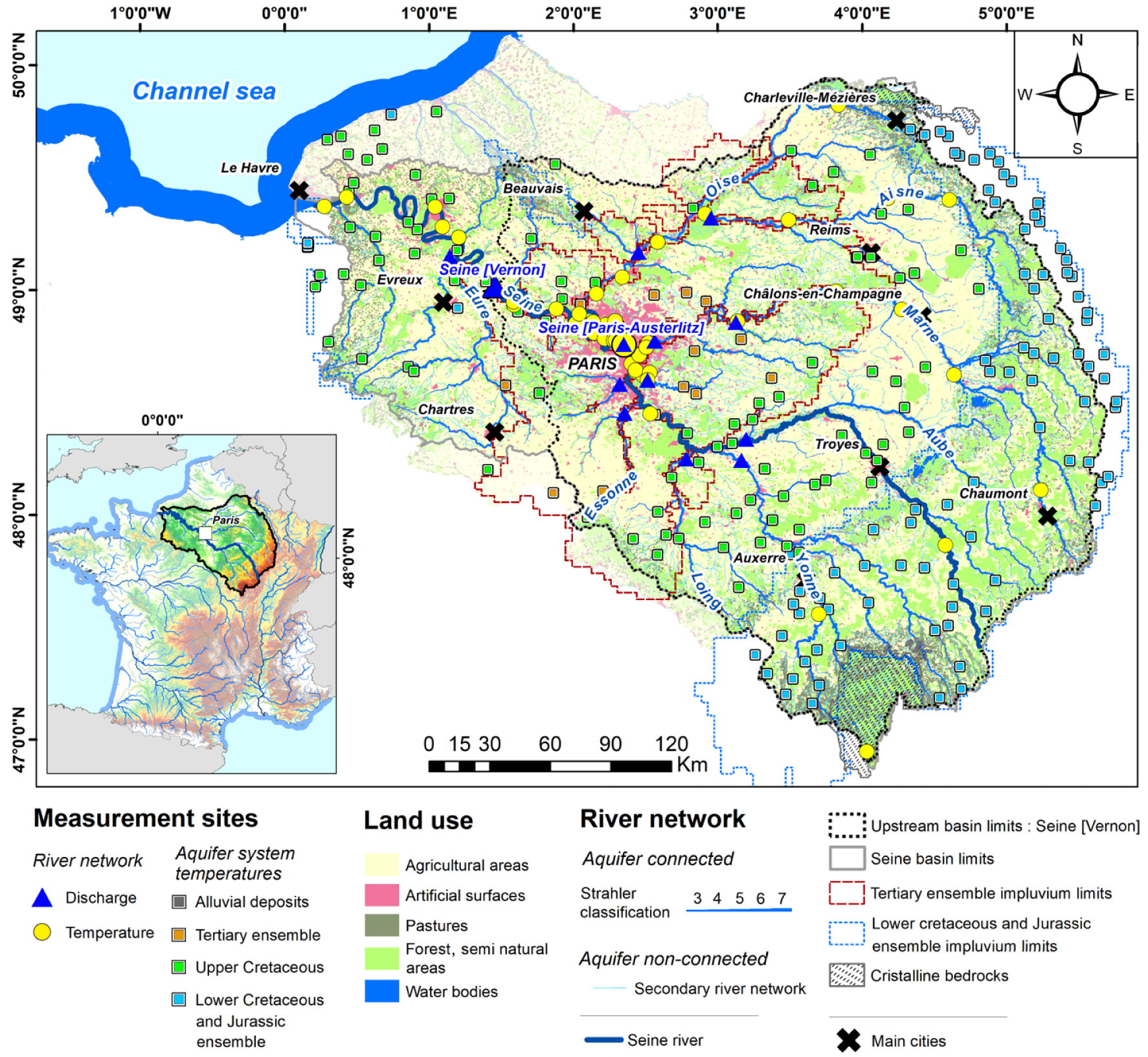
2.2. Numerical tools and model development
2.2.1. ORCHIDEE (tag 2.2, rev. 6533)
ORCHIDEE is a SVAT model, initially designed to be coupled to an atmospheric global circulation model [Krinner et al. 2005], but it can also be used in stand-alone mode, using an input meteorological data set. ORCHIDEE tag 2.2 was developed as part of the IPSL-CM6 model [Boucher et al. 2020] to contribute to the sixth phase of the Coupled Model Intercomparison Project (CMIP6) [Eyring et al. 2016].
The horizontal resolution is imposed by the atmospheric grid, and the energy and water budgets of the land surface are calculated in each grid-cell at a sub-hourly time step (15-min in the coupled model, 30-min in stand-alone mode) to properly account for the diurnal variations of incoming radiation. These budgets depend strongly on land cover, described in each grid-cell as a mosaic of 15 plant functional types (PFTs) including bare soil, evergreen and deciduous trees, C3 and C4 grasses and crops. All PFTs share the same equations but with different parameters. The proportion of each PFT is prescribed in each grid cell from land cover maps derived from satellite observations, with yearly updates [Lurton et al. 2020]. Two options are compared in this work regarding the evolution of leaf area index (LAI), which can be either prescribed via input maps of monthly LAI, or calculated dynamically at a daily time step by the so-called STOMATE module, which redistributes the net primary production (photosynthesis minus autotrophic respiration) owing to PFT dependent rules of allocation and phenology.
The vertical soil moisture redistribution is modelled by a multi-layer solution of Richards equation, using a 2-m soil discretized into 11 soil layers, with free drainage as a bottom boundary condition. Infiltration and infiltration-excess surface runoff are derived from a Green-Ampt parameterization [d’Orgeval et al. 2008]. The unsaturated values of hydraulic conductivity and diffusivity are given by the Van Genuchten–Mualem relationships. In each grid cell, the corresponding parameters (including saturated hydraulic conductivity Ksat and porosity) are deduced from soil texture as detailed in Tafasca et al. [2020]. Ksat (in m⋅s−1) further undergoes a vertical exponential decay to account for the effects of soil compaction and bioturbation:
| (1) |
Evapotranspiration is composed of four sub-fluxes: sublimation, interception loss, soil evaporation, and transpiration, tightly coupled to photosynthesis. Soil evaporation and transpiration depend on soil moisture via stress factors reducing the effective rates compared to the potential rate, which itself depends on an aerodynamic resistance (and stomatal resistance for transpiration) and the water vapor gradient between the surface and the atmosphere. Evapotranspiration E (in kg⋅m−2⋅s−1) and its energy equivalent, the latent heat flux LE (in W⋅m−2), couple the water and the energy budgets, calculated at the grid-cell scale given by:
| (2) |
2.2.2. CaWaQS (v3.17)
Mostly relying on the former MODCOU-NEWSAM software [Ledoux et al. 1989] based on the blueprints of de Marsily et al. [1978], the physically-based CaWaQS3.x [Flipo et al. 2022, 2007] computes, at a daily time-step, the main physical processes controlling the water budget and flow dynamics in each compartment of a hydrosystem. Each CaWaQS library deals with a specific compartment of a hydrosystem. This feature allows users to bypass certain modules when necessary and makes CaWaQS suitable for coupled applications.
CaWaQS is capable of distributing forcing fluxes over its own grid, and accepting forcing fluxes at various grid sizes. Forcing runoff fluxes are aggregated by CaWaQS to local sub-catchment areas and directly routed to the river network in which river discharges are simulated using a Muskingum scheme and water levels are simulated using a Manning–Strickler approach [Saleh et al. 2011]. Saturated groundwater flows are numerically solved using a finite difference solution of the 2-D diffusivity equation on a multi-layered nested grid. Vertical exchanges between aquifer layers and stream-aquifer exchanges depend on drainance and conductance concepts respectively i.e. a 1-D steady-state approach, assumed to be linearly linked to the head difference between two aquifer layers or river water level-aquifer head difference [Flipo et al. 2014]. Aquifer recharge from the unsaturated zone as well as anthropogenic withdrawals are treated as source terms.
Recent advances added a transport module, which simulates heat and solute transport in porous media (aquifer, pseudo-3D resolution) and the free surface compartment (river network, 1-D approach). Transport is described using the following advection-diffusion equation:
| (3) |
River-atmosphere heat exchanges are described based on an energy budget equation similar to (2) but for water temperature Tw; the various heat fluxes were calculated following Magnusson et al. [2012]. Whilst the energy income from the sun is the largest source of energy for a river system, clouds, riparian vegetation and topography-related shading can reduce heat input significantly [Loicq et al. 2018]. The limited permeability of aquitard layers constrains water flow to the vertical direction between aquifers [de Marsily 1986]. Similarly, streambed flow is also dominated by vertical exchanges between the stream and its underlying aquifer layer. Consequently, heat flow between two adjacent aquifers separated by an aquitard layer or a streambed linking the river with the aquifer layer can be resolved by a 1-D analytical solution. In this study, the heat exchanges through aquitard layers and streambed were resolved by the analytical solution of Kurylyk et al. [2017]:
| (4) |
The aquitard interface is a 3-layered system with 3 unknowns, i.e. the temperatures of the aquitard, as well as of the top and bottom aquifers. The streambed interface is a 2-layered system with 3 unknowns, i.e., the streambed, river and aquifer temperatures. The analytical solution coefficients are incorporated as a term of the solution matrix of the porous media, thereby simultaneously resolving the heat transport in the aquitard. The river temperature in the previous time-step is used to calculate the streambed temperature at the stream-aquifer interface. The streambed temperature calculated by the analytical solution is then used as the lower boundary of the river transport simulation. The developed transport module was validated using the analytical solution of Goto et al. [2005] [Kilic et al. 2021, Wang et al. 2021].
2.2.3. Model coupling strategy
Coupling is achieved via an “offline” forcing procedure, whereby the models involved are sequentially run, thus only allowing one-way interaction, from ORCHIDEE to CaWaQS. To this end, selected ORCHIDEE simulation results are used as daily CaWaQS upper boundary conditions: drainage fluxes simulated by ORCHIDEE are prescribed as CaWaQS aquifer recharge, with a temperature equal to the one in the soil at 2-m, while surface runoff is routed to the river system, assuming its temperature is at equilibrium with the soil surface temperature (0.001 m depth, top layer).
The correspondence between the ORCHIDEE grid mesh and the elementary surface units of CaWaQS is handled by CaWaQS, via spatially weighted area-based arithmetic means. The coupled model scheme internally projects each element to its geographic coordinate and then passes the forcing flux information to the receiving model.
2.2.4. Numerical experiment design
The coupled tool was applied over the 2001–2018 period, which was noteworthy for remarkable flood events (e.g. winter/spring 2001, winter 2016–2018) as well as extremely low-flow/drought periods and heat-waves (e.g. summer 2003, summer 2006–2007).
ORCHIDEE setup
ORCHIDEE is run over the Seine basin in stand-alone mode, forced with the SAFRAN meteorological data set [Vidal et al. 2010]. It provides the required atmospheric variables at an hourly time step, over a regular 8 × 8 km grid, which is therefore the horizontal resolution of the simulations. A total of 1490 cells are used to described the simulated domain. A constant carbon dioxide concentration (370 ppm) over the period 1980–2018 was applied.
The vegetation distribution map was derived at 0.5° resolution from the ESA-CCI Land Cover dataset at 300 m resolution, for the 1992–2015 period [see details in Lurton et al. 2020]. Vegetation distribution outside this period was set to that of the nearest available year with a constant vegetation distribution. For simulations with prescribed LAI, the monthly values were obtained from an existing 40-year global simulation performed in stand-alone mode at 0.5° (55 km resolution). The soil background albedo map was derived from the MODIS albedo dataset aggregated at 0.5° resolution. Soil texture distribution maps were obtained from four sources: Reynolds [Reynolds et al. 2000], SoilGrids [Hengl et al. 2017], LUCAS [Ballabio et al. 2016], and INRA [Jolivet et al. 2006]. The initial state was obtained after a five-year warm-up period (1980–1985) in order to reach the land surface model equilibrium state for soil moisture and soil temperature.
CaWaQS setup
A pre-existing CaWaQS application over the Seine basin, which considers the main aquifer units in interaction with the Seine river and its main tributaries [Flipo et al. 2022], was used here. From the oldest to the most recent, these aquifers can be grouped according to the following four main ensembles: (i) an ensemble of aquifer and aquitard units, ranging from Lower Jurassic (Hettangian stage) to Lower Cretaceous (Albian stage), (ii) the large Upper Cretaceous chalk aquifer, (iii) a Tertiary aquifer complex including the five main aquifer layers dating from Palaeocene to Miocene stages and (iv) recent alluvial deposits (Pleistocene, Holocene). The resolution of CaWaQS aquifer cells range between 100 m–3200 m using a nested-grid approach. River geometry was obtained from the SYRAH-CE [Chandesris et al. 2008] database. River network water inputs account for subsurface runoff, overflows from aquifer to soil surface as well as river–aquifer exchanges. Mainly due to computation time concerns, river–aquifer exchange calculations were restrained to the main hydraulic network, which corresponds to river reaches with a Strahler order above or equal to 3 (Figure 1). The thermal parameterization (thermal conductivities, heat capacities and porosities) of the Seine basin was extracted from Dentzer [2016] and Rivière [2012]. Heat transport was simulated in the river reaches with a Strahler order above or equal to 3 (Figure 1). Soil surface temperatures obtained from ORCHIDEE were prescribed to river reaches below Strahler order 3. The initial temperature state of the aquifer system was obtained by running the coupled model for 40 years by re-cycling 2 sets of 20-year simulations in the period 1985–2005.
CaWaQS forcings were defined as follows: (i) A no-flow boundary condition is imposed at the bottom and border limits of the domain, except where the mesh boundary corresponds to an adjacent river. (ii) Groundwater withdrawals are taken into account as a daily pumping rate, inferred from the annual groundwater abstraction data of the Seine basin water management agency (Agence de l’eau Seine-Normandie, AESN) for domestic, industrial and agricultural needs. (iii) Agricultural withdrawals are assumed to take place only during the summer period (i.e. bulk irrigation water volume is distributed as: 20% in May, 30% in June and July, and 20% in August). (iv) A no-heat flux boundary condition is imposed for the horizontal borders. (v) A Dirichlet boundary condition is assigned to the top boundary of the groundwater system for transport. (vi) Geothermal fluxes are assumed for the bottom limit of the domain [75 m⋅Wm−2, Dentzer 2016].
2.2.5. Calibration protocol
Calibration strategy
A two-step calibration procedure was used to calibrate the water and heat cycle of the Seine Hydrosystem. Considering the impact of North Atlantic Oscillation (NAO) on the groundwater and river stock variation [Flipo et al. 2012], a 17-year averaging period between 2001–2018 was selected to conduct the first step of the optimization procedure.
The surface hydrology calibration step consists of iterative trial-and-error adjustments of the ORCHIDEE parameters to minimize the bias between simulated and observed mean pluri-annual discharge at Vernon, the most downstream gauging station of the Seine before the estuary (Figure 1). The bias was calculated after the simulated pluri-annual mean discharge (estimated by total runoff times basin area) was corrected for yearly groundwater abstraction (annual average equivalent of 37 m3⋅s−1 during 2008–2012, AESN) from the basin. Previous studies [Flipo et al. 2022] indicate that around two-thirds of effective rainfall contributes to aquifer recharge in the basin, and this ratio was also considered as a qualitative target for the calibration.
A set of 10 ORCHIDEE simulations were chosen to illustrate this iterative process (Table 1). First, EXP1–EXP4 allow us to assess the influence of the soil texture map (with a prescribed LAI map and default parameters, as used at global scale for CMIP6). Then, the two available options to account for LAI variations (prescribed map vs dynamic simulation by the STOMATE module) can be assessed by comparing EXP4 and EXP5. Finally, EXP5–EXP10 only differ by some ORCHIDEE parameters found to be effective by several sensitivity analyses [e.g. Raoult et al. 2021]: the saturated hydraulic conductivity (Ksat) assigned to the dominant soil textures in the Seine River basin (loamy sand, loam, clay loam) and its decay factor cK (1); the visible and near-infrared leaf albedo and maximum LAI of the main PFTs in the basin. It must be noted that no calibration was carried out to improve the thermal fluxes. The temperatures of soil bottom and soil top layers were assumed to be at equilibrium with the recharge (drainage) and surface runoff temperatures, respectively.
Parameter set applied to the 10 experiments to calibrate the ORCHIDEE model
| Experiment | EXP1 | EXP2 | EXP3 | EXP4 | EXP5 | EXP6 | EXP7 | EXP8 | EXP9 | EXP10 | |
|---|---|---|---|---|---|---|---|---|---|---|---|
| Soil distribution | I | SG | L | R | R | R | R | R | R | R | |
| Vegetation model | pLAI | pLAI | pLAI | pLAI | ST | ST | ST | ST | ST | ST | |
| Parameter | Class | ||||||||||
| cK | 2 | — | — | — | — | 4 | — | — | 10 | — | |
| Ksat (m⋅s−1) | Loamy sand | 4.05 × 10⁻⁵ | — | — | — | — | — | — | 1.73 × 10⁻⁵ | — | — |
| Loam | 2.88 × 10⁻⁶ | — | — | — | — | — | — | 1.50 × 10⁻⁶ | — | — | |
| Clay loam | 7.22 × 10⁻⁷ | — | — | — | — | — | — | 4.62 × 10⁻⁷ | — | — | |
| Near-infrared leaf albedo | TeBE | 0.22 | — | — | — | — | — | 0.2 | — | — | — |
| TeBS | 0.22 | — | — | — | — | — | 0.2 | — | — | — | |
| NC3 | 0.3 | — | — | — | — | — | 0.25 | — | — | — | |
| AC3 | 0.3 | — | — | — | — | — | 0.1 | — | — | — | |
| Visible-light leaf albedo | TeBE | 0.06 | — | — | — | — | — | 0.04 | — | — | — |
| TeBS | 0.06 | — | — | — | — | — | 0.04 | — | — | — | |
| NC3 | 0.1 | — | — | — | — | — | 0.05 | — | — | — | |
| AC3 | 0.1 | — | — | — | — | — | 0.04 | — | — | — | |
| Maximum LAI | TeBE | 4.5 | — | — | — | — | — | — | — | — | 5.5 |
| TeBS | 4 | — | — | — | — | — | — | — | — | 5 | |
| NC3 | 2 | — | — | — | — | — | — | — | — | 3 | |
| AC3 | 2 | — | — | — | — | — | — | — | — | 3 | |
—: same value than the previous one, R: Reynolds, SG: SoilGrids, L: Lucas, I: INRA, pLAI: prescribed LAI, ST: STOMATE activated, TeBS: Temperature Boreal Summergreen Trees, TeBe: Temperate Boreal Evergreen Trees, NC3: Natural C3 grass, AC3: Agricultural C3 crops.
CaWaQS parameterizations of river network and groundwater were taken from the pre-calibrated parameter set provided by Flipo et al. [2022]. No additional calibration of the hydrological components and groundwater heat transport of CaWaQS were undertaken, but the river heat budget was calibrated by modifying the uniform shading factor ranging from 0% to 50% applied on the net incoming radiation on the river [Beaufort et al. 2016]. A 30% uniform shading, consistent with reported shading factor values [Loicq et al. 2018], was selected after a series of simulations.
Evaluation strategy
To validate the coupled model performance, the Seine basin hydrogeological and thermal application results were compared to a set of river discharge and water level monitoring wells as well as river and aquifer temperature data, distributed among the different aquifer units (Figure 1). The Kling–Gupta Efficiency coefficient (KGE), Root Mean Square Error (RMSE), Mean Absolute Error (MAE), Percent bias (PBIAS) and the Pearson correlation coefficient (CC) were used to quantitatively evaluate the misfit between simulated and observed values and dynamics.
Field data were collected between 2001–2018. The variables collected are discharge data from 183 gauging stations; hydraulic head data from 267 piezometers were used to evaluate the performance statistics of the hydrology part. Discharge and hydraulic head time series data were obtained from publicly available ADES and HYDRO national datasets. River water temperature data were assembled from various agencies operating in the basin; the dataset comprises hourly and daily observations from 62 sites [Rivière et al. 2021]. During the simulation period (2001–2018), 48 stations with hourly observations were selected. The aquifer temperature data used were obtained from the national ADES database. While providing a comprehensive amount of data, records are often incomplete and heterogeneous. The majority of the temperature data were collected on site while pumping, hence the depths of the temperature observations represent the depth of the screened well. A pre-processing was therefore applied to the dataset using the interquartile range (IQR) method, as described in Hemmerle et al. [2019]. From the initial data set of 9179 stations over the Seine-Normandy region, 212 stations with a minimum of 40 observations over the simulation period remained after the pre-processing.
3. Results and discussions
3.1. Calibration of the surface water cycle
The simulated water balance, shown in Figure 2, illustrates how the different parameter configurations (Table 1) influence the partitioning of the precipitation into actual evapotranspiration (AET), surface runoff and recharge (drainage). The first four simulations (EXP1-4) show the impact of the soil texture map, which induces a 6% variation of AET (mean values between 469 and 497 mm⋅a−1), also reflected in the total runoff (effective precipitation). Soil texture also impacts the partitioning of the total runoff between drainage and surface runoff, which varies between 20 and 47% of the total runoff between EXP4 (Reynolds) and EXP2 (SoilGrids), as the SoilGrids and INRA maps include a significant fraction of silty soils that increase the surface runoff at the expense of drainage [Tafasca et al. 2020]. Eventually, the Vernon discharge bias decreases from 39.8% in EXP1 to 25.9% in EXP4, so we kept the Reynolds soil texture map for further optimization.
Mean yearly surface water budget components calculated by ORCHIDEE in mm⋅a−1. Bias was calculated on the multi-year mean discharge at Vernon gauging station after the adjustments on the mean yearly water abstractions are taken into account for EXP1-10. CaWaQS column represents the water balance calculated by the CaWaQS-Seine application including water abstractions.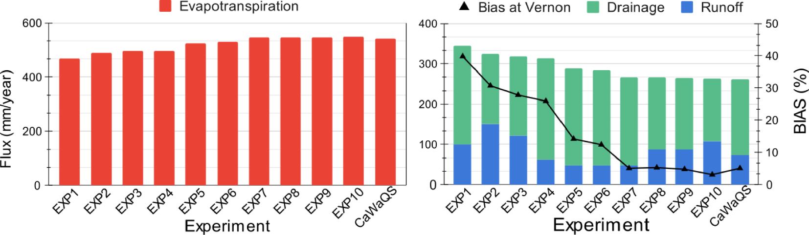
The dynamic calculation of the vegetation dynamics by the STOMATE module (EXP5) allows a further increase in AET (+26 mm⋅a−1) compared to simulations with prescribed LAI (EXP1-4). The reason is that STOMATE calculates a higher LAI than the prescribed one, increasing the AET via a larger biomass during the growth season. The resulting decrease in total runoff leads to a further reduction of the Vernon discharge bias decreases, from 25.9% to 14.2 %. The small decrease in the contribution of surface runoff to total runoff (−3%) can be attributed to the trade off between surface runoff and increased vegetation activity and water abstraction of roots in the topsoil. Reducing the NIR and VIS leaf albedo (from EXP6 to EXP7) also yielded a significant increase in AET (+16 mm⋅a−1, i.e. +5%), because it increases the net available energy. This brings a further reduction of the discharge bias at Vernon to 5.1% in EXP7.
In contrast, implementing a sharper vertical decay of Ksat below 30 cm in the soil column (from EXP5 to EXP6) showed a weak impact on all the studied variables: AET improved slightly by only 4 mm⋅a−1, the discharge bias by only 1.8%, the partition of the total runoff, and the surface runoff fraction was hardly changed. This weak sensitivity to modifications of the vertical Ksat profile shows the importance of the top 30 cm of the soil column on the water balance rather than deeper zones [De Rosnay et al. 2000]. The decrease of Ksat for all the dominant soil textures (EXP7–EXP8) had an even smaller impact on AET, total runoff thus on the discharge bias (even slightly worsened). Decreasing Ksat, however, showed a significant impact on the partition of total runoff, as it nearly doubled the contribution of surface runoff (from 18% to 33%). The additional decrease of Ksat in the bottom part of the soil by increasing the decay factor cK to 10 (EXP9) had no impact on the water and energy budget, and the increase of maximum LAI (EXP 10) had a very limited effect on AET and total runoff although it increased the proportion of surface runoff (+10%). The maximum LAI values in all simulations including EXP10 match the reported LAI ranges observed throughout the FluxNET network for similar biomes and climates [Krinner et al. 2005]. A detailed calibration of vegetation properties is beyond the scope of this study, although ways to improve the terrestrial biosphere and energy processes in SVAT models are active research domains [Peylin et al. 2016].
Eventually, these results show that the overestimation of discharge at the Vernon outlet resulted from an underestimated AET. A considerable improvement of the discharge bias came from the dynamic LAI calculations, which may partly be attributed to the coarse resolution of the input LAI map in pLAI simulations, and to a better seasonal cycle of LAI (comparison to GiMMS [Zhu et al. 2013] product not shown), more consistent with the SAFRAN meteorological forcing. Although groundwater withdrawals are taken into account in the calculation of the ORCHIDEE discharge bias (see Section 2.2.5), the lack of irrigation in the simulations may also contribute to the underestimation of AET and the overestimation of river discharge since the enhancement of AET by surface water withdrawals is overlooked. Considering that ORCHIDEE simulates a natural basin contrary to heavily regulated and irrigated Seine basin, a 3.1% bias (EXP10) at the outlet of the basin (Vernon) is very satisfactory. However, when the proportions of infiltration and surface runoff are considered (see Section 2.2.5), EXP9 performs better with nearly two-thirds of recharge contributing to total runoff.
3.2. Performance of the ORCHIDEE-CaWaQS coupled simulation
The best performing ORCHIDEE simulation in terms of river discharge bias and partitioning of effective rainfall (EXP9) was selected to force the CaWaQS simulation. A coupled simulation was performed over the 17 year period (August 2001–July 2018). The simulated discharge compared satisfactorily with observed stream flow in 14 main sub-catchments, as illustrated at the outlet of the Seine basin (Vernon) in illustrated in Figure 3a. Although low flows are slightly overestimated by the coupled model, it captures the yearly dynamics properly (KGE = 0.77, CC = 0.82) and mean volume (PBIAS = 1.6%), given that the measurement error of river discharge can reach 20% [Sauer and Meyer 1992].
Comparison between (a) simulated (red) and observed (blue) discharge at the outlet of Seine watershed (Vernon); (b) simulated (red) and observed (blue) river temperature at Paris (Austerlitz). From August 2001 to July 2018. Years indicate 1st of January. KGE: Kling–Gupta Efficiency coefficient; CC: Correlation Coefficient; PBIAS: Percent Bias; RMSE: Root Mean Square Error.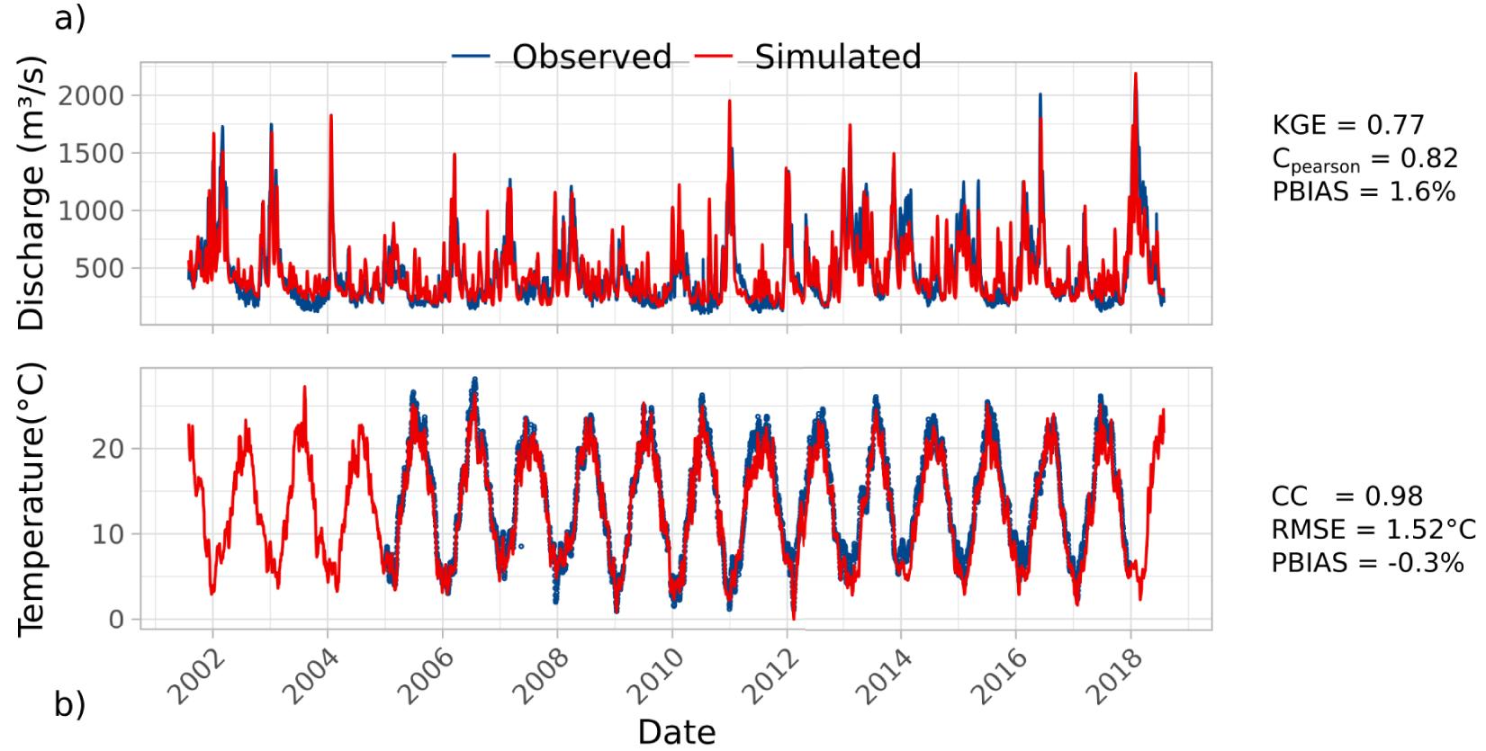
Stream temperature is also well simulated along the Seine basin, as illustrated by Paris-Austerlitz station (Figure 3b). The simulated temperatures match the observed ones (CC = 0.98) with a PBIAS of −0.3% and an RMSE of 1.52 °C, although simulated temperatures are generally underestimated in both summer and winter. Part of this uncertainty can be attributed to the uniform shading factor or the lack of urban structures that artificially modifies the heat regime on riverbanks [Ferguson and Woodbury 2007]. The model also uses a uniform and time-constant shading factor which deviates from the prevalent seasonal dynamics and spatial distribution of the vegetation in the Seine basin (Figure 1). Model performances respectively evaluated against stream and aquifer temperature probes over the simulation period are provided in Tables 2 and 3.
Statistical criteria (2001–2018 period) from 48 stream temperature probes distributed in the basin
| Value range (°C) | RMSE | MAE | RMSE | MAE |
|---|---|---|---|---|
| Station count (-) | Cumulative percentage (%) | |||
| [0.0–2.0[ | 31 | 42 | 65 | 88 |
| [2.0–4.0[ | 15 | 1 | 96 | 90 |
| [4.0–6.0[ | 2 | 2 | 100 | 94 |
| [6.0–8.0[ | 0 | 3 | 100 | 100 |
| Value range (-) | CC | KGE | CC | KGE |
| Station count (-) | Cumulative percentage (%) | |||
| ]0.7–1.0] | 48 | 43 | 100 | 90 |
| ]0.5–0.7] | 0 | 2 | 100 | 94 |
| ]0.4–0.5] | 0 | 1 | 100 | 96 |
| ]0.2–0.4] | 0 | 2 | 100 | 100 |
Upper table: Root Mean Square Error (RMSE), Mean Absolute Error (MAE). Lower table: Pearson correlation coefficient (CC), and Kling–Gupta Efficiency (KGE) coefficient.
Statistical criteria (2001–2018 period) from 212 aquifer temperature probes distributed in the basin
| Value range (°C) | RMSE | MAE | RMSE | MAE |
|---|---|---|---|---|
| Piezometer count (-) | Cumulative percentage (%) | |||
| [0.0–2.0[ | 93 | 115 | 44 | 54 |
| [2.0–4.0[ | 58 | 37 | 71 | 72 |
| [4.0–6.0[ | 16 | 16 | 79 | 79 |
| [6.0–8.0[ | 17 | 16 | 87 | 87 |
| [8.0–10.0[ | 8 | 9 | 91 | 91 |
| ⩾10 | 20 | 19 | 100 | 100 |
RMSE: Root Mean Square Error, MAE: Mean Absolute Error.
The dynamics of the heat transport in the river network is well represented (CC > 0.7 for 100% of the stations) and MAE is lower than 2 °C for 88% of the stations. 96% of the river temperature stations have an RMSE lower than 4 °C. Water temperatures at streams and small rivers (<10,000 km2) show a higher mean RMSE (2.58 °C) than downstream (⩾10,000 km2) stations (1.58 °C). Prescribed temperatures on river reaches with a Strahler order below 3 strongly influence the river temperatures on streams and small rivers and contribute to the higher RMSE because the proportion of reaches with a prescribed temperature is higher than downstream reaches. A relatively high RMSE indicates a misfit between simulated and observed temperatures at the daily scale. Overall the seasonal dynamics are well represented in the river network (Figure 3b). Heat transport in the river performs comparably to other studies at the regional scale using the equilibrium temperature method [Beaufort et al. 2016] in terms of RMSE.
The groundwater temperatures show a good fit as the RMSE is below 2 °C for 44% of the stations. The median RMSE calculated for the aquifer observations was 2.12 °C (ranging between 20.2 and 0.01 °C). Stations with a larger than 10 °C RMSE are focused on the Jurassic aquifer. This is largely due to a mismatch between the depth of the well and the depth of the cell. However, only 22% of the stations show a CC higher than 0.5. Only 3% of the stations show a KGE performance greater than 0.5. The limiting factor in terms of the dynamics is the lack of sufficient time series in the aquifer system. Regarding the assumptions for the estimates of the upper boundary conditions for heat transport in the groundwater system, simulated soil temperatures at 2 m depth from ORCHIDEE were applied to the groundwater system top boundary, which are quite different from the actual temperatures of groundwater at the water table [Anderson 2005].
4. Hydrological and thermal functioning of the Seine hydrosystem
The results of the best ORCHIDEE-CaWaQS simulation were used to compute the water budget (Figure 4) and the energy budget (Figure 5) of the whole Seine basin, including groundwater contributions, over the period 2001–2018.
Water budget of the Seine hydrosystem over the period 2001–2018 as simulated by ORCHIDEE-CaWaQS application. Groundwater system encompasses the full extent of the aquifers. ITB: Infiltration flux for outcropping aquifer units beyond the Seine basin limits. Flows outside boundaries (OTB) are beyond the extent of the Seine basin. Flows are expressed in inter-annual average values in m3⋅s−1. Rainfall = 760 mm⋅a−1, AET∗ = 559 mm⋅a−1, Runoff = 69 mm⋅a−1, Infiltration = 132 mm⋅a−1. Model layers: “Alluvium”: Alluvial deposits, “Beauce”: Beauce limestones ensemble, “Brie”: Brie limestones and Fontainebleau sands, “Champigny”: Champigny limestones, “Lutetian”: Lutetian limestones, “Thanetian”: Thanetian sands, “Chalk”: Upper Cretaceous chalk aquifer, “JLC. ens.”: Lower Cretaceous and Jurassic ensemble.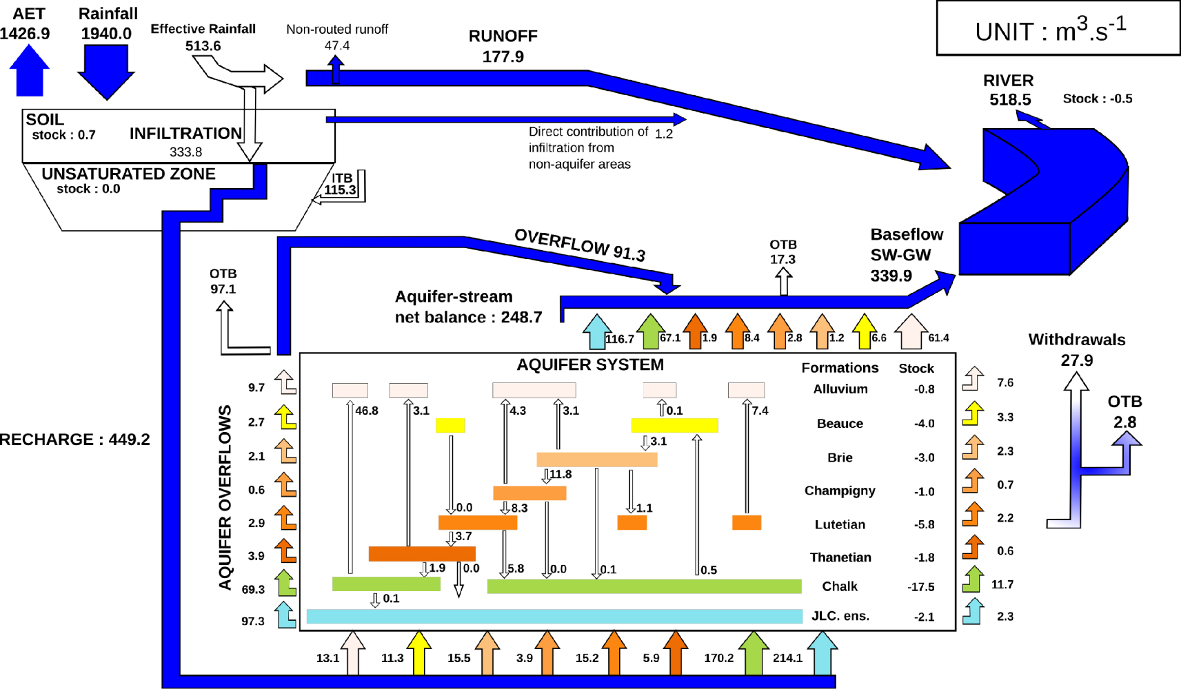
Heat budget of the Seine hydrosystem over the period 2001–2018 as simulated by ORCHIDEE-CaWaQS application. Groundwater system encompasses the entire aquifer extents. Flows outside boundaries are beyond the extent of the Seine basin. Energy amounts are expressed in multi-annual average values in GWh per day and mean annual daily air temperature and soil temperature at 2 m depth are shown in °C. 𝛥 Heat: net thermal load variation in the river network. SW: net short-wave radiation, LW: long-wave radiation, SH: sensible heat, LH: latent heat. Model layers: “Alluvium”: alluvial deposits, “Beauce”: beauce limestones ensemble, “Brie”: Brie limestones and Fontainebleau sands, “Champigny”: Champigny limestones, “Lutetian”: Lutetian limestones, “Thanetian”: Thanetian sands, “Chalk”: upper Cretaceous chalk aquifer, “Jurassic”: lower Cretaceous and Jurassic ensemble.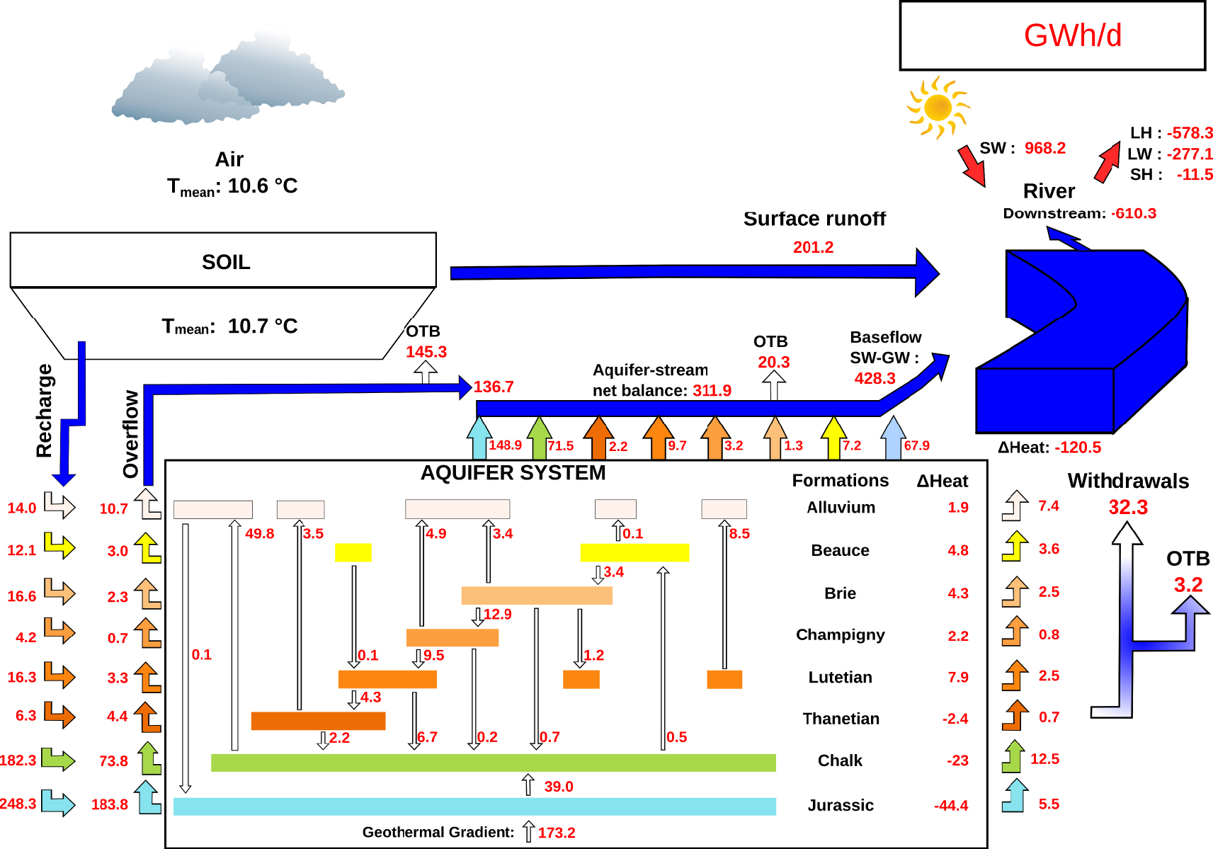
4.1. Pluri-annual water budget
Figure 4 displays a pluri-annual water budget of the Seine basin. The AET represents 73.5% (559 mm⋅a−1) of the rainfall (760 mm⋅a−1). The remaining effective rainfall (201 mm⋅a−1) is partitioned into surface runoff and groundwater recharge, amounting to 34.6% and 65.3% of the effective rainfall, respectively. A total infiltration flow of 449.2 m3⋅s−1 transits through the unsaturated zone, recharging the whole aquifer system. 27.8% of the aquifer recharge is lost through regional water fluxes across the Seine basin boundaries (21.6% of recharge) or withdrawn from the system by pumpings (6.2% of recharge). Within the Seine basin, river–aquifer exchanges for Strahler orders higher than 3 supply roughly half of the discharge (248.7 m3⋅s−1) recorded at the outlet of the river network (Figure 4). What is called overflow mostly corresponds to the drainage of the groundwater system by low Strahler orders (one and two). It therefore also corresponds to stream-aquifer exchanges, and amounts to 91.3 m3⋅s−1 (17.6% of total discharge). Finally, surface runoff contributes up to 177.9 m3⋅s−1 (34.4% of total discharge).
4.2. Pluri-annual heat budget
The pluri-annual heat budget over the period 2001–2018 is illustrated in Figure 5. The pluri-annual average temperature of the air is 10.6 °C in the Seine basin, and the pluri-annual average temperature of the soil surface is 11.3 °C (i.e. the temperature associated to surface runoff). Soil temperature at 2 m depth is estimated as 10.7 °C. The mean daily river temperature is estimated as 12.1 °C (Figure 5). Yearly mean aquifer temperatures range between 10.6 °C for the shallow alluvium aquifer and 23.8 °C for the deeper Jurassic aquifer. The largest heat gains in the aquifer system are due to the recharge fluxes (182.5 TWh) and the geothermal gradient (63.2 TWh) at the bottom of the basin (Figure 5). The former represents advective fluxes while the latter represents conductive fluxes. The influence of advection diminishes with depth as expected, while conduction becomes the dominant thermal process. This is due to the decrease of water fluxes with depth.
The main sources of surface advective heat losses are due to: (i) river–aquifer exchanges (113.8 TWh), (ii) stream-aquifer exchanges for the secondary river network (Strahler orders 1 and 2) (i.e. overflow that amounts 102.9 TWh), (iii) and withdrawals (11.8 TWh). The aquifer system looses the most energy via the Jurassic, the Chalk and the alluvium aquifers. The Jurassic loses the largest advective heat fluxes via overflow and river–aquifer exchanges towards the surface (Figure 5). The Chalk aquifer and the alluvium are the second and third largest contributors to river via advective term. The Chalk aquifer is also the largest contributor to thermal losses due to water withdrawal (4.6 TWh).
Energy from short-wave radiation (net radiation, 353.4 TWh) is main non-advective source of heat gain in the river network annually (Figure 5), contributing 60% of the river thermal load during the study period. As evidenced in Figure 4, the river–aquifer exchanges for the simulated river (Strahler orders larger than 3) and overflow (Strahler orders 1 and 2) are the largest contributors to the river heat budget. The incidence of the hydrological regime on the heat balance in the river network is illustrated by the large advective heat flux via baseflow (156.3 TWh per year), which forms the second source of river heat gains. Surface runoff contributes 13% of the total thermal load in the river network. The largest non-advective heat losses in the river network are latent heat and long-wave radiation losses, accounting for 67% (211.0 TWh) and 32% (101.1 TWh), respectively. Approximately 1% of total heat losses are due to sensible heat losses in the river.
4.3. Seasonal heat fluxes in the river network
Seasonal variations of each term of the heat balance in the river network are provided in Table 4. It is important to note that the heat exchanges between river and aquifer is not simulated by the model for the rivers with a Strahler orders lower than 3. This implies that the fluxes are not calculated on the same river extent as the other terms. Short-wave radiation is higher during summer and spring. It depends on the sunlight reaching to stream surface, albedo of water, and shading factor which limits the sunlight. The shading factor can vary as a function of stream morphology, riparian vegetation, urban structures, or clouds [Loicq et al. 2018]. Although a fixed shading factor was used in this study (30%), more work is needed to implement the shading factor’s spatial variability due to the aforementioned factors. The order of non-advective heat sinks does not vary seasonally, as latent heat is the largest heat sink in the system, followed by long-wave radiation, sensible heat and streambed conduction, respectively. Latent heat causes on average a 120.6 W⋅m−2 heat loss during summer and 20.3 W⋅m−2 heat loss during winter. From the simulation, heat fluxes related to conduction in the streambed are negligible when compared to other flux terms, regardless of the season.
Seasonal heat fluxes (W⋅m−2) in the Seine river network over the 2001–2018 period
| Process | Type | Winter | Spring | Summer | Autumn | Average |
|---|---|---|---|---|---|---|
| Short-wave radiation | Conductive | 39.3 | 142.0 | 180.1 | 75.9 | 109.3 |
| Long-wave radiation | Conductive | −16.1 | −42.9 | −44.6 | −21.5 | −31.3 |
| Latent heat | Conductive | −20.3 | −69.9 | −120.6 | −50.4 | −65.3 |
| Sensible heat | Conductive | −0.2 | −1.7 | −2.1 | −1.1 | −1.3 |
| Streambed conduction | Conductive | 0.4 | −0.2 | −0.7 | −0.1 | 0.2 |
| Surface runoff | Advective | 13.3 | 18.9 | 37.9 | 20.8 | 22.7 |
| Streambed advection | Advective | 54.0 | 54.8 | 44.3 | 39.5 | 48.1 |
| Net gains | — | 69.1 | 101.5 | 96.2 | 63.2 | 82.5 |
The total river length is 28,378 km. The total surface area of the river network with Strahler order higher than 3 is 369 km2. The streambed fluxes are the heat exchanges between river and aquifer. Net gains is the heat balance of the river network. Negative sign (−) indicates loosing fluxes by the river.
Seasonally, heat gains in the Seine river are mainly controlled by the short-wave radiation and river–aquifer exchanges. During winter the net heat gains related to short-wave radiation decrease to only 22% of the heat gains during the summer period (Table 4). River–aquifer exchanges sustain the heat gains of the river network throughout seasons, and become the dominant heat source during winter. Advective heat flux contributions by each aquifer unit change every season due to river and riverbed temperature variations and the magnitude of the river–aquifer exchanges. Studies usually assume that the riverbed conduction contribution is negligible with respect to the advective heat input [Magnusson et al. 2012]. Our study confirms this statement as riverbed conduction reaches up to only 1.5% of river–aquifer advective fluxes.
Loinaz et al. [2013] has showed that at the catchment scale, river–aquifer exchanges contribute to a significant fraction of heat sources. Similarly, in the Seine basin, river–aquifer exchanges contribute significantly to the river energy budget. Locally, the river–aquifer exchanges can dominate the heat balance especially during the winter (Table 4). This can create a local cooling effect during summer or a warming effect during winter; an essential aspect of the river–aquifer exchanges that creates thermal refugia for fish species [Kaandorp et al. 2019]. Also, local thermal variations in the river have implications for the industrial use of water and pollution [Prest et al. 2016].
Although a detailed sensitivity analysis was not feasible within the scope of this paper, a similar study at the regional scale in the Loire Basin reported that the dominant factors, in decreasing order of importance, were the shading factor, headwater temperatures, groundwater flow, discharge and river geomorphology, respectively [Beaufort et al. 2016]. Our approach differs from this study, which relied on an equilibrium temperature concept, by the way that the processes are treated explicitly and streambed temperature is estimated by an analytical solution in a distributed manner. We found that the river-atmosphere exchange had the largest impact on the river heat balance at regional scale.
4.4. Implications on the water–energy–food nexus
Water, food, and energy are the three essential elements that is needed for human survival and livelihood [De Amorim et al. 2018]. The Water–Energy–Food Nexus (WEFN) has emerged since the early 2010’s as a new approach to collectively manage three finite resources, whose accessibility is increasingly threatened by climate change, population growth, urbanization, and environmental concerns [Hoff 2011]. The need for a nexus approach has been motivated by the fact that there is a competition for water between water, food and energy production.
Our study shows that the Jurassic aquifer (Figure 5) has a good potential for the geothermal use. This fact is well known, the Dogger aquifer (part of the Jurassic aquifer) is exploited for more than 40 years via low temperature geothermal energy applications [Lopez et al. 2010]. The Paris basin has a great potential for geothermal energy production as annual thermal energy recycling is substantial (182.5 TWh via recharge and 63.2 TWh via geothermal gradient annually). For comparison, France produced 548.6 TWh electricity in 2020 [NEA 2020]. Our findings indicate that the geothermal energy potential to offset part of this energy production is substantial. Further research is needed to assess the suitability of aquifer thermal energy systems (ATES) applications at shallower depths [Lee 2010] in the Seine River basin.
Our coupled ORCHIDEE-CaWaQS model therefore opens the way for new research that integrates the WEFN in the sense that it can be used to assess the impact of energy and agricultural policies at the basin scale in a quantitative way, leveraging on previous studies describing the effect of agricultural practices on the Seine hydro-agrosystem with the ancestor of CaWaQS [Beaudoin et al. 2018].
5. Conclusions and perspectives
A first coupling model of water and energy fluxes at the regional scale (96,204 km2) was carried out with a focus on the Seine hydrosystem in order to address the hydrological and thermal functioning of the hydrosystem and quantify the interactions between surface and subsurface compartments. The distribution of the thermal loads in the Seine hydrosystem including the aquifer system and the river network at the regional scale is quantified for the first time.
Overall, the coupled framework simulates the mean discharge at various sub-catchment scales in the Seine basin and hydraulic heads in the groundwater system adequately for the purposes of thermal transport simulation. For a first attempt of such a coupling between a SVAT (ORCHIDEE) and a hydrological model (CaWaQS), the platform performs satisfactorily for the simulation of both water fluxes and energy fluxes. The coupled ORCHIDEE-CaWaQS framework is designed to take advantage of broadly available gridded datasets from catchment to regional scales to estimate hydrosystem water and energy budgets. The transport module estimated the mean river temperatures and aquifer temperatures adequately.
The findings presented herein have the potential to inform biological or water quality studies [Flipo et al. 2020] on the Seine basin or engineering applications such as ATES to reduce the dependency on fossil fuel [Lee 2010] by providing insights into key physical processes driving the heat fluxes in the river network and the aquifer system. The impact of climate change on the share of energy fluxes at the regional basin scale will also be studied and provide useful information for adaptation and mitigation strategies. The model, for example, can be integrated in an ecohydrological model to estimate the impacts of thermal variability on fish or riparian habitat [Loinaz et al. 2014]. These efforts can have policy implications by guiding environmental management agencies to prioritize their restoration and exploitation areas in the Seine basin. Future coupling with an agronomic model [Beaudoin et al. 2018] will also provide a complete picture within the WEFN framework [Garcia and You 2016] at the regional scale, thereby improving our understanding of the competing aspects of limited resources.
Conflicts of interest
The authors declare no competing financial interest.
Dedication
The manuscript was written through contributions of all authors. All authors have given approval to the final version of the manuscript. DK: designed the research, developed the CaWaQS transport module, performed all simulations, analyzed the data and prepared the manuscript draft. AR: designed the research, developed CaWaQS transport module, designed the transport through streambed and aquitard interfaces, interpreted results, discussed findings, contributed and improved the manuscript. NG: developed the CaWaQS transport module and the required CaWaQS coupling functionalities, contributed to figures and improved the manuscript. SW: developed the CaWaQS transport module. AD: contributed to the design of the ORCHIDEE application, interpreted ORCHIDEE results and discussed findings. PP: contributed to the design of the ORCHIDEE application, interpreted ORCHIDEE results and discussed findings. NF: designed the research, managed the development of CaWaQS, interpreted results, discussed findings and improved the manuscript, managed and ensured the funding of the project.
Acknowledgments
This work is a contribution to the PIREN Seine research program, which is part of the Zone Atelier Seine, included in the e-LTER network. We gratefully acknowledge the river temperature dataset provided by William Thomas. Groundwater withdrawals were obtained from Seine-Normandy Water Agency, over the 1994–2012 period. We would like to thank two anonymous reviewers for their input that improved the final article’s quality.