Impact of integration time steps of rain drop size distribution on their double-moment normalization: a case study in northern Benin

Sounmaïla Moumouni; Fulgence Payot Akponi; Eric-Pascal Zahiri; Agnidé Emmanuel Lawin; Marielle Gosset

doi:10.5802/crgeos.200

Atmospheric Sciences

Impact of integration time steps of rain drop size distribution on their double-moment normalization: a case study in northern Benin

Sounmaïla Moumouni ¹ ; Fulgence Payot Akponi ^1,² ; Eric-Pascal Zahiri ³ ; Agnidé Emmanuel Lawin ⁴ ; Marielle Gosset ⁵

¹Ecole Normale Supérieure (ENS) de Natitingou, Université Nationale des Sciences, Technologies, Ingénierie et Mathématiques (UNSTIM), Bénin
²Département Physique, Faculté des Sciences et Techniques; Université d’Abomey-Calavi, Bénin
³Laboratoire des Sciences de la Matière, de l’Environnement et de l’Energie Solaire, Université Félix Houphouët-Boigny, Côte d’Ivoire
⁴Laboratoire d’Hydrologie Appliquée (LHA), Institut National de l’Eau (INE), Université d’Abomey-Calavi, Benin
⁵Géosciences-Environnement-Toulouse (GET), Institut de Recherche pour le Développement (IRD), France

Comptes Rendus. Géoscience, Volume 355 (2023), pp. 109-133

Abstract

This study analyzed the sensitivity of the double-moment normalization of rain drop size distributions (DSDs) to their integration time steps. Six DSD datasets measured at different integration time steps were modeled by the double-moment normalization method. Six couples of reference moments are used for the normalization. Three DSD models (gamma, generalized gamma and lognormal) are used for modeling. Statistical criteria are used to assess the estimation of the moments of the DSDs made by the models. As results, the analysis highlighted the dependence of the shape function parameters on the DSD integration time step. It is also noted that the three DSD models are well adapted to the data used. Nevertheless, the generalized gamma model is recommended because of the independence of the moment estimation errors with respect to the integration time step, which is not the case for the other models.

Metadata

Article information
Cite this article

Received: 2022-06-02
Revised: 2022-10-20
Accepted: 2023-01-12
Published online: 2023-02-01

DOI: 10.5802/crgeos.200

Keywords: Rain DSD, Double-moment normalization, Integration time steps, Unimodal DSD models, Generalized gamma, Weather radars, West Africa rainfall

Author's affiliations:

Sounmaïla Moumouni ¹ ; Fulgence Payot Akponi ^{1
,

2} ; Eric-Pascal Zahiri ³ ; Agnidé Emmanuel Lawin ⁴ ; Marielle Gosset ⁵

¹ Ecole Normale Supérieure (ENS) de Natitingou, Université Nationale des Sciences, Technologies, Ingénierie et Mathématiques (UNSTIM), Bénin
² Département Physique, Faculté des Sciences et Techniques; Université d’Abomey-Calavi, Bénin
³ Laboratoire des Sciences de la Matière, de l’Environnement et de l’Energie Solaire, Université Félix Houphouët-Boigny, Côte d’Ivoire
⁴ Laboratoire d’Hydrologie Appliquée (LHA), Institut National de l’Eau (INE), Université d’Abomey-Calavi, Benin
⁵ Géosciences-Environnement-Toulouse (GET), Institut de Recherche pour le Développement (IRD), France

License:

CC-BY 4.0

Copyrights: The authors retain unrestricted copyrights and publishing rights

Sounmaïla Moumouni; Fulgence Payot Akponi; Eric-Pascal Zahiri; Agnidé Emmanuel Lawin; Marielle Gosset. Impact of integration time steps of rain drop size distribution on their double-moment normalization: a case study in northern Benin. Comptes Rendus. Géoscience, Volume 355 (2023), pp. 109-133. doi: 10.5802/crgeos.200

@article{CRGEOS_2023__355_G1_109_0,
     author = {Sounma{\"\i}la Moumouni and Fulgence Payot Akponi and Eric-Pascal Zahiri and Agnid\'e Emmanuel Lawin and Marielle Gosset},
     title = {Impact of integration time steps of rain drop size distribution on their double-moment normalization: a case study in northern {Benin}},
     journal = {Comptes Rendus. G\'eoscience},
     pages = {109--133},
     year = {2023},
     publisher = {Acad\'emie des sciences, Paris},
     volume = {355},
     doi = {10.5802/crgeos.200},
     language = {en},
}

TY  - JOUR
AU  - Sounmaïla Moumouni
AU  - Fulgence Payot Akponi
AU  - Eric-Pascal Zahiri
AU  - Agnidé Emmanuel Lawin
AU  - Marielle Gosset
TI  - Impact of integration time steps of rain drop size distribution on their double-moment normalization: a case study in northern Benin
JO  - Comptes Rendus. Géoscience
PY  - 2023
SP  - 109
EP  - 133
VL  - 355
PB  - Académie des sciences, Paris
DO  - 10.5802/crgeos.200
LA  - en
ID  - CRGEOS_2023__355_G1_109_0
ER  -

%0 Journal Article
%A Sounmaïla Moumouni
%A Fulgence Payot Akponi
%A Eric-Pascal Zahiri
%A Agnidé Emmanuel Lawin
%A Marielle Gosset
%T Impact of integration time steps of rain drop size distribution on their double-moment normalization: a case study in northern Benin
%J Comptes Rendus. Géoscience
%D 2023
%P 109-133
%V 355
%I Académie des sciences, Paris
%R 10.5802/crgeos.200
%G en
%F CRGEOS_2023__355_G1_109_0

Original version of the full text (Propose a translation )

The full text below may contain a few conversion errors compared to the version of record of the published article.

1. Introduction

Modeling rain Drop Size Distributions (DSDs) is useful for several applications such as: (i) the quantitative estimation of rainfall by weather radars or by mobile telecommunication links; (ii) predicting the attenuation of satellite signals by rain; (iii) washing of atmospheric particles by rain; (iv) soil erosion by rain; etc. This modeling aims to parameterize the rain DSD by a minimum number of scale parameters that can be related to the meteorological variables observed by sensors—for instance radar reflectivity. Inspired by several previous works, Sempere-Torres et al. [1994, 1998] proposed a general single-moment normalization to formulate the DSD in terms of a scaling law. Later, based on the work of Testud et al. [2001], Lee et al. [2004] proposed a general double-moment normalization approach to the DSD. Using convective and stratiform DSD data, they showed that double-moment normalization better captures the natural variability of the DSDs than single-moment normalization. In terms of physical interpretation, the scaling exponent of the single-moment normalization has a marked dependence on the type of rain i.e., with microphysical processes inducing the raindrop formation, whereas in the double-moment normalization distinction between rain type is not necessary [Lee et al. 2004].

The analysis of the impact of DSD integration time step on their modeling began with the work of Chapon et al. [2008]. Recently, using single-moment normalization (scale parameter: rain intensity), Moumouni et al. [2021] highlighted the dependence of the shape function parameters of DSD models (gamma and lognormal) on the DSD integration time step. By fitting the individual spectra with unimodal DSD models (gamma and lognormal), they also showed that the overall proportion of well-fitted and very well-fitted spectra increases with the integration time step. The need to integrate DSD measurement in time (or space, with a network of disdrometers) is related to the very small sampling area of disdrometers [Tapiador et al. 2017] which leads to sampling error in individual spectra estimation. The amount of integration is a tradeoff between avoiding random errors due to sampling errors and the risk to smooth up too much the part of DSD variability that is related to microphysical processes (such as convective/stratiform).

For polarimetric radar, several authors [Bringi et al. 2003, 2006, Gorgucci et al. 2002, Gosset et al. 2010, Testud et al. 2001] have shown the importance of the double-moment normalization of the DSD. Indeed, the double-moment normalization of DSD provides an excellent model to reduce the DSD variability which strongly affects radar rain retrieval algorithms since this approach is quite effective in collapsing the DSDs around a mean shape. This work aims to analyze the impact of the DSD integration time step on their double-moment normalization. For this purpose, the double-moment normalization of the DSD approach, proposed by Lee et al. [2004], will be used and applied to DSD data measured in northern Benin [Moumouni et al. 2008, 2021]. Thus, the following sections will be devoted successively to the datasets, the method, the results and discussions, and the concluding remark.

2. Datasets

The DSDs data used for this study are those sampled in northern Benin, near the town of Djougou (9.66°N, 1.69°E)—using optical Disdrometers: single beam [Löffler-Mang and Joss 2000, Salles 1995, Salles et al. 1998] and double beam [Delahaye et al. 2005]—from 2005 to 2007, during the African Monsoon Multidisciplinary Analysis (AMMA) meteorological campaign. The climate of the study area is mainly characterized by a unimodal rainfall regime with April to October as period of the unique rainy season. The annual rainfall is about 1200 mm but is marked by a downward trend on the last decades. The DSDs data have been validated and widely used for several studies [Gosset et al. 2010, Kougbéagbédé et al. 2017, Moumouni 2009, Moumouni et al. 2008, 2018]. These data are DSDs of rains with an integration time step equal to one minute. They are made up of 93 rainy events which represent a total of: 11,647 spectra when only rain intensities greater than or equal to 0.1 mm⋅h⁻¹ are considered; and 12,342 spectra for a threshold of to 0.05 mm⋅h⁻¹. The selected rainy events are isolated at the level of each Disdrometer. A rainy event is defined as event with duration at least equal to 15 min and intermittency less than 30 min. The duration of the selected rainy events varies from 15 to 527 min.

From these data, Moumouni et al. [2021] computed other rain DSDs datasets of various integration time steps (Table 1). The DSDs duration T = L min (L = 1,2,3,4,…,20) were calculated within each event, and the remaining spectra whose number is less than L are not taken into account.

Data	DATA1	DATA2	DATA3	DATA4	DATA5	DATA6
Integration time steps	T = 1 min	T = 2 min	T = 5 min	T = 10 min	T = 15 min	T = 20 min
Number of spectra	12,342	6152	2437	1198	777	578
Cumulative (mm)	1237.16	1236.89	1235.53	1225.94	1217.20	1216.79

3. Methods

Since the pioneering work of Marshall and Palmer [1948] on the rain Drop Size Distribution (DSDs), most of followed studies [Atlas et al. 1999, Cerro et al. 1997, Chen et al. 2019, Tenorio et al. 2012, Tokay and Short 1996, Uijlenhoet et al. 2003, Ulbrich 1983, Ulbrich and Atlas 1998, Wen et al. 2018, Willis 1984, Zeng et al. 2019, Zhang et al. 2003, etc.] analysed it with N(D) function defined by spectrum of a given period T (generally 1 min is used). The diameter of drop named equivalent diameter is the diameter of the sphere having the same volume as that of the measured drop. N(D) corresponds to the number of raindrops per unit of volume and by interval of diameters and is calculated as follows:

N (D_{r}) = \frac{N_{r}}{S T Δ D_{r} V (D_{r})}

(1)

where r is the index of the class of equivalent diameter, ΔD_r the width of the range of equivalent diameter centred on D_r. In this study, D_r and ΔD_r are expressed in millimeters. S is the disdrometer collecting surface area expressed in square meter. For the sampling period T, N_r is the number of drops counted by the disdrometer in each size range. V (D_r) is the falling speed of the drops of diameter D_r. For the rain intensity to be proportional to a moment of N(D) function, the relationship between the drops speed and their diameter is used as suggested by Atlas and Ulbrich [1977]:

V (D_{r}) = 3.78 D_{r}^{0.67} (m \cdot s^{- 1}) .

(2)

In all the above studies, T = 1 min = 60 s and N(D_r) is expressed in (m⁻³⋅mm⁻¹).

The measured moment of order n of a rain DSD spectrum (whatever the integration time steps) is defined [Chapon et al. 2008, Lee et al. 2004, Ochou et al. 2007, Sempere-Torres et al. 1994, Zeng et al. 2019] by

M_{mea, n} = \sum_{r} D_{r}^{n} N (D_{r}) Δ D_{r} with n ⩾ 0 and n \neq \infty .

(3)

When we assume a DSD model, the theoretical moment of order n of a rain DSD spectrum (whatever the integration time steps) is defined [Chapon et al. 2008, Lee et al. 2004, Ochou et al. 2007, Sempere-Torres et al. 1994, Zeng et al. 2019] by

M_{n} = \int_{0}^{+ \infty} D^{n} N (D) d D with n ⩾ 0 and n \neq \infty .

(4)

3.1. Double-moment normalization [Lee et al. 2004]

There are several variants of DSD normalization that can be summarized in two approaches: single-moment normalization and double-moment normalization. The single-moment normalization method was generalized by Sempere-Torres et al. [1994]. The double-moment approach was generalized by Lee et al. [2004]. The latter proved that the DSD can be normalized by any two of its reference moments (M_i and M_j, i≠j). This is how they linked the function N(D) to a the normalizing function which we named the shape function F(x) and to two parameters D_c and N_c (with x = D∕D_c), such that

N (D) = N_{c} F (\frac{D}{D_{c}}) .

(5)

The parameters D_c and N_c are defined according to the moments M_i and M_j (with i≠j)

D_{c} = {(\frac{M_{j}}{M_{i}})}^{\frac{1}{j - i}}

(6)

and

N_{c} = M_{i}^{\frac{j + 1}{j - i}} M_{j}^{- \frac{i + 1}{j - i}} .

(7)

When N(D) is expressed in (m⁻³⋅mm⁻¹), we note that the moments of order nM_mea,n or M_n are expressed in (m⁻³⋅mmⁿ) and therefore the parameters D_c and N_c are expressed respectively in (mm) and (m⁻³⋅mm⁻¹). Thus, the parameters D_c and N_c stand for the average size and the concentration of the drops in the DSD spectrum, respectively. When we introduce the expression (5) in (4), we get

M_{n} = C_{n} N_{c} D_{c}^{n + 1}

(8)

with

C_{n} = \int_{0}^{+ \infty} x^{n} F (x) d x .

(9)

Substituting (6) and (7) in (8) we obtained

M_{n} = C_{n} M_{i}^{\frac{j - n}{j - i}} M_{j}^{- \frac{i - n}{j - i}} .

(10)

The self-consistency of the constant C_n are obtained by successively setting n = i and n = j in expression (10). Thus, this leads to C_i = 1 and C_j = 1.

The choice of the two reference moments depends on the use of DSD modeling. In the following, to facilitate the understanding of this modeling, we have chosen two reference moments of successive order by posing i = k and j = k + 1, with k⩾0 and k≠∞. Thus, the expressions (6), (7) and (10) become

\begin{matrix} D_{c} & = & \frac{M_{k + 1}}{M_{k}} \end{matrix}

(11)

\begin{matrix} N_{c} & = & \frac{M_{k}^{k + 2}}{M_{k + 1}^{k + 1}} \end{matrix}

(12)

and

M_{n} = C_{n} M_{k}^{k - n + 1} M_{k + 1}^{n - k} .

(13)

The self-consistency of the constant C_n corresponds in this case to: C_k = 1 and C_k+1 = 1.

3.2. Case of the gamma DSD model

The gamma DSD model proposed by Tokay and Short [1996] or Maki et al. [2001] is written

N (D) = N_{G} D^{𝜇} exp (- 𝛬_{G} D)

(14)

N_G, 𝛬_G and 𝜇 are the model parameters: N_G is the intercept parameter; 𝛬_G is the slope parameter; and 𝜇 is the shape parameter. Its theoretical moment of order n, calculated with formula (4) is

M_{n} = N_{G} \frac{𝛤 (𝜇 + n + 1)}{𝛬_{G}^{(𝜇 + n + 1)}} .

(15)

In this expression, 𝛤 is the mathematical function gamma. By calculating the moments M_k and M_k+1 with expression (15) and replacing them in expressions (11) and (12), we find

𝛬_{G} = \frac{𝜇 + k + 1}{D_{c}}

(16)

and

N_{G} = \frac{N_{c} {(𝜇 + k + 1)}^{(𝜇 + k + 1)}}{D_{c}^{𝜇} 𝛤 (𝜇 + k + 1)} .

(17)

Substituting (16) and (17) into (14), and taking into account the expression (5), one obtains the expression the shape function of the gamma DSD model

F_{G} (x; 𝜇) = \frac{{(𝜇 + k + 1)}^{(𝜇 + k + 1)}}{𝛤 (𝜇 + k + 1)} x^{𝜇} exp [- (𝜇 + k + 1) x] .

(18)

By calculating (9) with the expression (18), this leads to the following relationship.

C_{G, n} = \frac{{(𝜇 + k + 1)}^{(k - n)} 𝛤 (𝜇 + n + 1)}{𝛤 (𝜇 + k + 1)} .

(19)

3.3. Case of the generalized gamma DSD model

Similarly to the gamma DSD model (14), the generalized gamma DSD model can be written in this form

N (D) = N_{GG} D^{𝜈} exp (- 𝛬_{GG} D^{𝜀})

(20)

N_GG, 𝛬_GG, 𝜈 and 𝜀 are the model parameters: N_GG is the intercept parameter; 𝛬_GG is the slope parameter; and 𝜈 and 𝜀 are the shape parameters. Its theoretical moment of order n, calculated with formula (4) is

M_{n} = N_{GG} \frac{𝛤 [(𝜈 + n + 1) ∕ 𝜀]}{𝜀 𝛬_{GG}^{[(𝜈 + n + 1) ∕ 𝜀]}} .

(21)

By calculating the moments M_k and M_k+1 with expression (21) and replacing them in expressions (11) and (12), we find

𝛬_{GG} = {\{\frac{𝛤 [(𝜈 + k + 2) ∕ 𝜀]}{D_{c} 𝛤 [(𝜈 + k + 1) ∕ 𝜀]}\}}^{𝜀}

(22)

and

N_{GG} = \frac{𝜀 N_{c}}{D_{c}^{𝜈} 𝛤 [(𝜈 + k + 1) ∕ 𝜀]} {\{\frac{𝛤 [(𝜈 + k + 2) ∕ 𝜀]}{𝛤 [(𝜈 + k + 1) ∕ 𝜀]}\}}^{(𝜈 + k + 1)} .

(23)

Substituting (22) and (23) into (20), and taking into account the expression (5), leads to express the shape function of the generalized gamma DSD model as:

\begin{matrix} F_{GG} (x; 𝜈, 𝜀) & = & \frac{𝜀}{𝛤 [(𝜈 + k + 1) ∕ 𝜀]} \\ \times {\{\frac{𝛤 [(𝜈 + k + 2) ∕ 𝜀]}{𝛤 [(𝜈 + k + 1) ∕ 𝜀]}\}}^{(𝜈 + k + 1)} \\ \times x^{𝜈} exp \{- {[\frac{𝛤 [(𝜈 + k + 2) ∕ 𝜀]}{𝛤 [(𝜈 + k + 1) ∕ 𝜀]}]}^{𝜀} x^{𝜀}\} . \end{matrix}

(24)

By calculating (9) with the expression (24), one obtains

C_{GG, n} = {\{\frac{𝛤 [(𝜈 + k + 2) ∕ 𝜀]}{𝛤 [(𝜈 + k + 1) ∕ 𝜀]}\}}^{(k - n)} \frac{𝛤 [(𝜈 + n + 1) ∕ 𝜀]}{𝛤 [(𝜈 + k + 1) ∕ 𝜀]} .

(25)

∙ Comparison with the generalized gamma of Lee et al. [2004]

The generalized gamma DSD model proposed by Lee et al. [2004] is written as follows:

N (D) = M_{0} \frac{c 𝜆}{𝛤 (𝜇)} {(𝜆 D)}^{c 𝜇 - 1} exp (- {(𝜆 D)}^{c}) .

(26)

By comparing this expression to the expression (20), we notice that c =𝜀 and 𝜇 = (𝜈+1)∕c. By replacing these relations in the expression of the constant C_GG,2,n established by Lee et al. [2004] and setting i = k and j = k + 1, we find the expression of the constant C_GG,n (25). So models (20) and (26) are similar.

3.4. Case of the lognormal DSD model

The lognormal DSD model proposed by Feingold and Levin [1986] is written

N (D) = \frac{N_{T}}{\sqrt{2 π} D ln 𝜎} exp [- \frac{{ln}^{2} (D ∕ D_{g})}{2 {ln}^{2} 𝜎}]

(27)

N_T, D_g and 𝜎 are the parameters of the model: N_T the total drops number per unit volume (N_T = M₀); D_g is the geometric mean of drops diameter (

ln D_{g} = \bar{ln D}

); and 𝜎 geometric standard deviation (

{ln}^{2} 𝜎 = \bar{{(ln D - ln D_{g})}^{2}}

). ln is natural logarithm. Its theoretical moment of order n, calculated with formula (4) is

M_{n} = N_{T} D_{g}^{n} exp (\frac{1}{2} n^{2} {ln}^{2} 𝜎) .

(28)

By calculating the moments M_k and M_k+1 with expression (28) and replacing them in expressions (11) and (12), we find

D_{g} = D_{c} exp [- 0.5 (2 k + 1) {ln}^{2} 𝜎]

(29)

and

N_{T} = N_{c} D_{c} exp [0.5 k (k + 1) {ln}^{2} 𝜎] .

(30)

When we introduce (29) and (30) into (27) and take into account the expression (5), we obtain the expression the shape function of the lognormal DSD model

\begin{matrix} F_{L} (x; 𝜎) & = & \frac{exp [0.5 k (k + 1) {ln}^{2} 𝜎]}{\sqrt{2 π} x ln 𝜎} \\ \times exp \{- \frac{{[ln x + 0.5 (2 k + 1) {ln}^{2} 𝜎]}^{2}}{2 {ln}^{2} 𝜎}\} . \end{matrix}

(31)

By calculating (9) with the expression (31), we obtain

C_{L, n} = exp \{0.5 [k^{2} + n^{2} + k - n (2 k + 1)] {ln}^{2} 𝜎\} .

(32)

3.5. Implementation of double-moment normalization

For each rain DSD integration time step, the double-moment normalization is implemented successively as follows:

Calculation of the sample moments of order n with (3).
Choice of two reference moments of order k and k + 1, then the calculation of the parameters D_c and N_c and of the average sample of C_n with the relation (8).
Estimation of the parameters of each shape function. The constant C_n being used at the end of the modeling to estimate the moments, these sample will be used to estimate the parameters of the shape functions.
1. For the gamma DSD model, the parameter 𝜇 is estimated by making a least-squares adjustment by comparing C_G,n (19) with the sample of C_n calculated in the previous step.
2. For the generalized gamma DSD model, the parameters 𝜈 and 𝜀 is estimated by making a least-squares adjustment by comparing C_GG,n (25) with the sample of C_n calculated in the previous step.
3. For the lognormal DSD model, the parameter 𝜎 is estimated by making a least-squares adjustment by comparing C_L,n (32) with the sample of C_n calculated in the previous step.
Calculation of the normalized spectra with the expression (5) then representation of these spectra and of the shape functions (gamma, generalized gamma and lognormal).
Model evaluation: comparison of the estimated moments M_est,n (8) with the measured moments M_mea,n (3). In expression (8), the constant C_n is estimated for each model from the estimated values of the parameters of the shape functions: C_G,n for the gamma model; C_GG,n for the generalized gamma model; and C_L,n for the lognormal model. For the comparison, the following statistical criteria were used:
In these expressions, E[⋅] denotes the sample mean.

4. Results and discussion

4.1. Results

The rain DSDs observed in northern Benin are modeled using the method above described. Data from the six integration time steps (Table 1) are used separately. For each integration time step, six different couples of moments (M_k, M_k+1) are used for normalization. The statistics of the parameters D_c and N_c, for each integration time step and for each couple of moments, are presented in Table A1 of the appendix. The average values of the constant C_n, for each integration time step and for each couple of moments, are presented in Table A2 of the appendix. The variation of these statistics between the couples of moments is obvious from expressions (11) and (12). Nevertheless, for a couple of moments, the variation of these statistics as a function of the integration time step is not obvious. This raises several questions: (i) are these statistics significantly different? (ii) if yes, what is this due to? These questions deserve to be addressed in our future work.

For the couple of moments (M₃, M₄), the result of the adjustment of the constant C_n, for each model, is represented in Figure 1. For the same couple of moments, the normalized spectra and the shape functions are represented in Figure 2. These figures show that each considered model fits well the DSDs observed in northern Benin. Figure 2 shows that: (i) the gamma and generalized gamma models seem to better model the mean distribution in the left tail; (ii) the three models seem to model the mean distribution in the same way in the intermediate region; (iii) the lognormal model seem to better model the mean distribution in the right tail. This description deserves to be deepened by first clarifying the importance of this mean distribution for the DSD modeling. Indeed, in this study, we adjusted the mean of the constant C_n instead of the mean distribution, because it is very useful for the estimation of the other moments from the reference moments (relation 10 and 13). Figure 1 shows that the constant C_n is better fitted by the generalized gamma model.

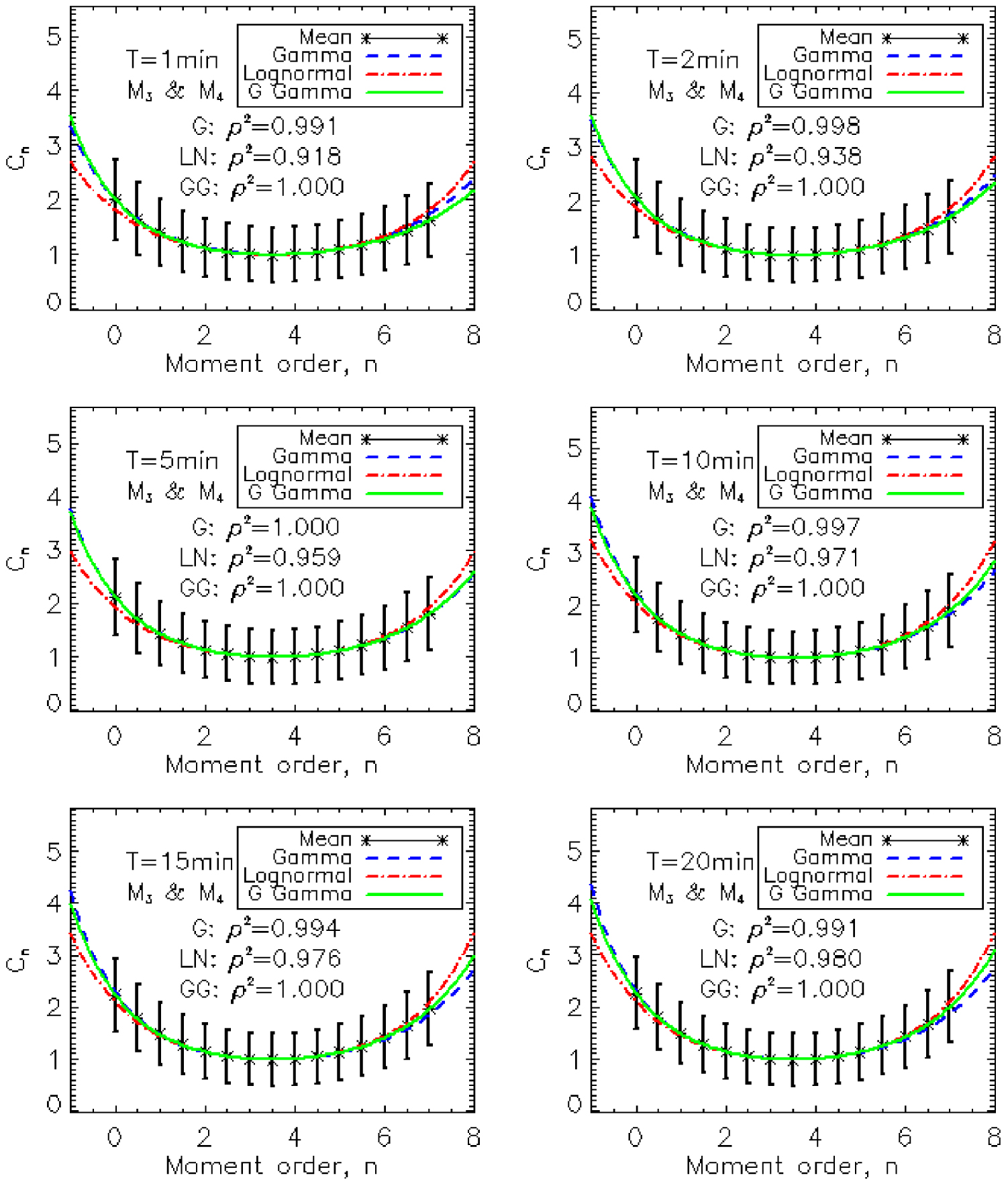
Figure 1.
Fit of the constant C_n for each model (G is gamma: blue, GG is generalized gamma (noted G Gamma): green and LN is lognormal: red). The asterisk represents the sample mean and the error bar represents the standard deviation. 𝜌² is the square of the linear Pearson correlation coefficient, between the sample mean and the model. Case of the couple of moments (M₃, M₄).

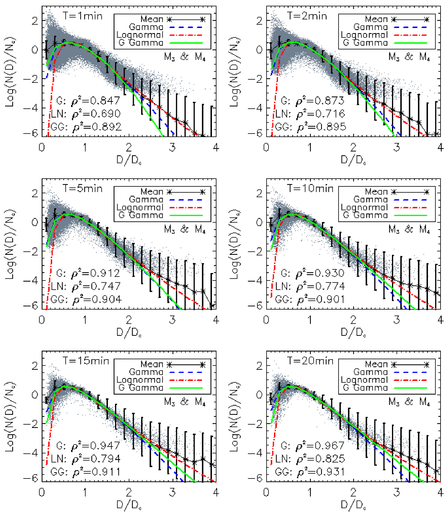
Figure 2.
Normalized spectra (slate gray dots) and the shape functions of the models (G is gamma: blue, GG is generalized gamma (noted G Gamma): green and LN is lognormal: red). The asterisk represents the sample mean and the error bar represents the absolute value of standard deviation. 𝜌² is the square of the linear Pearson correlation coefficient, between the sample mean and the model. Case of the couple of moments (M₃, M₄).

The importance of a DSD model being its ability to estimate from the reference moments its other moments, the three proposed models were evaluated. The result of this evaluation for the couple of moments (M₃, M₄) is shown in Figure 3. This result for the other couples of moments is shown in Figures A1 to A5, in the appendix. The SDFE indicates, for each couple of moments (M_k, M_k+1), whatever the integration time step, that the three models estimate the moments of order between k − 0.5 and k + 1.5 with almost null error. Nevertheless, this error becomes very significant outside this interval. The MRE indicates, for all couples of moments, that the estimate with the generalized gamma model is better than that of the other two models. Moreover, with the generalized gamma model, the MRE is almost independent of the integration time step, contrary to the case of the other two models.

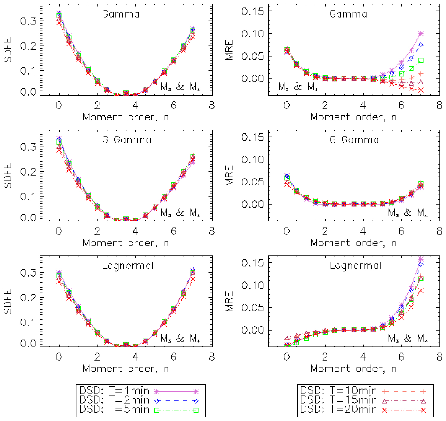
Figure 3.
Comparison of moments estimated to moments measured with SDFE and MRE. Case of the couple of moments (M₃, M₄), relating to the DSD models gamma, generalized gamma (noted G Gamma) and lognormal.

The impact of the integration time step on the modeling is analyzed. The estimated parameters, for each integration time step and for each couple of moments, are presented in Table 2. For the couple of moments (M₃, M₄), these parameters are represented as a function of the integration time step in Figure 4. The relationships established for the six couples of moments are presented in Table 3. The parameters of the shape functions are therefore dependent on the integration time step, whatever the model and the pair of moments.

T (min)	(M₀, M₁)				(M₁, M₂)				(M₂, M₃)
T (min)	𝜇	𝜈	𝜀	𝜎	𝜇	𝜈	𝜀	𝜎	𝜇	𝜈	𝜀	𝜎
1	6.040	3.520	1.470	1.400	6.190	2.650	1.680	1.380	6.550	3.680	1.400	1.360
2	5.750	4.360	1.220	1.410	5.780	3.620	1.340	1.390	5.920	4.610	1.160	1.370
3	5.560	5.000	1.080	1.410	5.510	4.250	1.180	1.390	5.550	5.290	1.030	1.380
4	5.440	5.440	1.000	1.420	5.360	5.040	1.040	1.400	5.340	5.620	0.970	1.380
5	5.350	5.910	0.930	1.420	5.230	5.480	0.970	1.400	5.150	6.140	0.900	1.390
6	5.250	6.460	0.860	1.420	5.090	5.790	0.920	1.410	4.970	6.630	0.840	1.390
7	5.150	6.660	0.830	1.430	4.980	6.390	0.850	1.410	4.850	6.740	0.820	1.390
8	5.100	7.050	0.790	1.430	4.920	6.780	0.810	1.410	4.750	7.160	0.780	1.400
9	5.070	7.380	0.760	1.430	4.860	7.090	0.780	1.410	4.670	7.640	0.740	1.400
10	4.960	7.630	0.730	1.430	4.720	7.460	0.740	1.420	4.510	7.750	0.720	1.400
11	4.910	7.990	0.700	1.430	4.670	7.990	0.700	1.420	4.440	7.990	0.700	1.410
12	4.840	8.190	0.680	1.440	4.580	8.190	0.680	1.420	4.340	8.190	0.680	1.410
13	4.830	7.730	0.710	1.440	4.590	7.710	0.710	1.420	4.360	7.710	0.710	1.410
14	4.780	8.430	0.660	1.440	4.520	8.630	0.650	1.420	4.270	8.450	0.660	1.410
15	4.720	8.680	0.640	1.440	4.450	8.890	0.630	1.430	4.180	8.700	0.640	1.410
16	4.700	9.010	0.620	1.440	4.430	9.250	0.610	1.430	4.160	8.660	0.640	1.410
17	4.630	9.070	0.610	1.440	4.340	9.310	0.600	1.430	4.050	8.900	0.620	1.420
18	4.620	9.250	0.600	1.450	4.330	9.730	0.580	1.430	4.030	9.070	0.610	1.420
19	4.550	9.980	0.560	1.450	4.230	10.530	0.540	1.430	3.900	10.030	0.560	1.420
20	4.590	9.610	0.580	1.450	4.290	10.140	0.560	1.430	3.990	9.230	0.600	1.420

T (min)	(M₃, M₄)				(M₄, M₅)				(M₅, M₆)
	𝜇	𝜈	𝜀	𝜎	𝜇	𝜈	𝜀	𝜎	𝜇	𝜈	𝜀	𝜎

1	5.930	3.050	1.570	1.370	6.170	3.920	1.340	1.380	6.600	3.500	1.460	1.350
2	5.650	3.990	1.270	1.380	5.750	4.900	1.110	1.390	5.970	4.480	1.190	1.370
3	5.480	4.640	1.120	1.380	5.490	5.490	1.000	1.390	5.610	5.020	1.070	1.380
4	5.380	5.200	1.020	1.390	5.330	5.960	0.930	1.400	5.380	5.470	0.990	1.380
5	5.220	5.750	0.940	1.390	5.190	6.320	0.880	1.400	5.190	5.960	0.920	1.390
6	5.110	6.300	0.870	1.400	5.060	6.720	0.830	1.410	5.010	6.530	0.850	1.390
7	5.030	6.620	0.830	1.400	4.950	6.960	0.800	1.410	4.880	6.750	0.820	1.390
8	4.990	7.160	0.780	1.400	4.890	7.410	0.760	1.410	4.770	7.150	0.780	1.400
9	4.940	7.500	0.750	1.400	4.830	7.620	0.740	1.410	4.700	7.640	0.740	1.400
10	4.810	7.750	0.720	1.410	4.690	7.890	0.710	1.420	4.550	7.750	0.720	1.400
11	4.780	8.320	0.680	1.410	4.640	8.140	0.690	1.420	4.460	8.300	0.680	1.410
12	4.700	8.360	0.670	1.410	4.560	8.350	0.670	1.420	4.370	8.530	0.660	1.410
13	4.690	8.030	0.690	1.410	4.560	7.860	0.700	1.420	4.390	8.200	0.680	1.410
14	4.650	8.810	0.640	1.410	4.500	8.620	0.650	1.420	4.300	8.610	0.650	1.410
15	4.580	8.880	0.630	1.420	4.430	8.890	0.630	1.420	4.210	8.870	0.630	1.410
16	4.580	9.460	0.600	1.420	4.420	8.680	0.640	1.420	4.170	9.010	0.620	1.410
17	4.490	9.520	0.590	1.420	4.310	9.100	0.610	1.430	4.070	9.280	0.600	1.420
18	4.500	9.950	0.570	1.420	4.310	9.520	0.590	1.430	4.040	9.680	0.580	1.420
19	4.410	10.520	0.540	1.420	4.220	9.820	0.570	1.430	3.930	10.220	0.550	1.420
20	4.470	10.120	0.560	1.420	4.290	9.260	0.600	1.430	4.010	9.860	0.570	1.420

𝜇: gamma, (𝜈,𝜀 ): generalized gamma, 𝜎: lognormal.

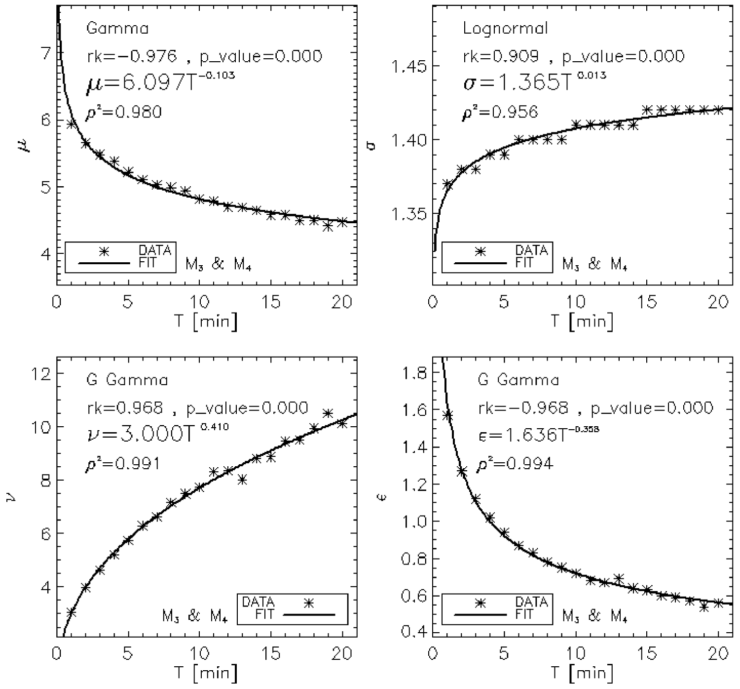
Figure 4.
Link between shape function parameters and integration time step. rk is the Kendall rank correlation between sample and integration time step. p_value is the significance level of the correlation. It’s in the interval [0.0,1.0]; a small value indicates a significant correlation. Case of the couple of moments (M₃, M₄). 𝜌² is the square of the linear Pearson correlation coefficient, between the sample and the model. Generalized gamma is noted G Gamma.

	Gamma				Lognormal
Couples	rk	p_value	Relationship	𝜌²	rk	p_value	Relationship	𝜌²
(M₀, M₁)	−0.989	0.000	𝜇 = 6.180T^−0.098	0.983	0.912	0.000	𝜎 = 1.396T^0.012	0.936
(M₁, M₂)	−0.979	0.000	𝜇 = 6.349T^−0.129	0.987	0.909	0.000	𝜎 = 1.375T^0.013	0.956
(M₂, M₃)	−0.979	0.000	𝜇 = 6.714T^−0.173	0.992	0.923	0.000	𝜎 = 1.356T^0.015	0.966
(M₃, M₄)	−0.976	0.000	𝜇 = 6.097T^−0.103	0.980	0.909	0.000	𝜎 = 1.365T^0.013	0.956
(M₄, M₅)	−0.984	0.000	𝜇 = 6.313T^−0.129	0.989	0.903	0.000	𝜎 = 1.376T^0.012	0.953
(M₅, M₆)	−0.979	0.000	𝜇 = 6.778T^−0.175	0.992	0.923	0.000	𝜎 = 1.352T^0.016	0.975

	Generalized gamma
Couples	rk	p_value	Relationship	𝜌²	rk	p_value	Relationship	𝜌²

(M₀, M₁)	0.968	0.000	𝜈 = 3.449T^0.343	0.989	−0.968	0.000	𝜀 = 1.527T^−0.321	0.994
(M₁, M₂)	0.968	0.000	𝜈 = 2.640T^0.450	0.990	−0.968	0.000	𝜀 = 1.753T^−0.377	0.994
(M₂, M₃)	0.947	0.000	𝜈 = 3.708T^0.314	0.979	−0.966	0.000	𝜀 = 1.427T^−0.294	0.994
(M₃, M₄)	0.968	0.000	𝜈 = 3.000T^0.410	0.991	−0.968	0.000	𝜀 = 1.636T^−0.358	0.994
(M₄, M₅)	0.937	0.000	𝜈 = 3.959T^0.294	0.984	−0.947	0.000	𝜀 = 1.359T^−0.280	0.995
(M₅, M₆)	0.968	0.000	𝜈 = 3.447T^0.353	0.991	−0.976	0.000	𝜀 = 1.513T^−0.325	0.994

They are established for the six couples of moments studied. rk is the Kendall rank correlation between sample and integration time step. p_value is the significance level of the correlation. It’s in the interval [0.0,1.0]; a small value indicates a significant correlation. 𝜌² is the square of the linear Pearson correlation coefficient, between the sample and the model.

4.2. Discussion

In West Africa, gamma and lognormal DSD models are used more to adjust measured DSDs [Nzeukou et al. 2004, Ochou et al. 2007, Sauvageot and Lacaux 1995, Moumouni et al. 2008, 2021]. This study showed that these models are well adapted for the analyzed DSDs, but the generalized gamma DSD model is better because of its flexibility [Lee et al. 2004].

The choice of reference moments for DSD normalization must be made according to the applications. In this article, we have analyzed the case of consecutive moment order, because it allows us to simplify the equations. The expressions of the shape function or the constant C_n, established for the three DSD models used, will be used for any application requiring the use of consecutive moment order. For other combinations of moments, one can refer to Lee et al. [2004]. For retrieval of rain intensity from radar measurements, these authors suggest the combination of moments M₆ (close to the reflectivity, variable measured by the radar) and M_i (i less than 6).

Weather radar measurements are usually based on a sequence of quasi-horizontal scans (PPIs, for Plan Position Indicators) each providing a quasi-instantaneous snapshot of the rain, with a typical sampling rate of 1 to 5 min. Depending on the overall scanning strategy, several subsequent PPIs may be used to provide a time averaged rainrate every 10 to 15 min. The parameters of the rainfall estimation algorithms or of DSD model are often derived from DSDs sampled at ground level, at 1 min time step. The results of this study can be used to transform these parameters to the time step most relevant for the application.

This article shows trends in the evolution of the shape parameters with respect to the DSD integration time step, in West Africa, as shown by Moumouni et al. [2021] with the single-moment normalization method. Unfortunately, to our knowledge, no reference relating to the study of the impact of the DSD integration time step on their double-moment normalization is available to make a comparison with. Meanwhile, it opens up other scientific questions: (i) do the trends in parameters values change from one climatic region to another? (ii) what is the physical significance of these changes? or more broadly, what is the cause of the variability of the shape parameters during the rainfall event? etc. All these important scientific questions for the modeling of the DSD, can be the subject of other works. The gamma, generalized gamma and lognormal models doesn’t have the same heavy tails [Halliwell 2013] as shown in Figure 2. For future work, we will consider this aspect, as well as the fitting of other models (Pareto and inverse gamma) by other methods [Halliwell 2013].

5. Concluding remark

Following the work of Moumouni et al. [2021] on the analysis of the impact of the integration time step on the single-moment normalization of the DSD, this study analyzes the impact of the integration time step on the double-moment normalization of the DSD. The method proposed by Lee et al. [2004] was used. It was applied to rain DSD data measured in northern Benin (West Africa) during AMMA intensive period experiment. DSD models gamma, generalized gamma, and lognormal are used for spectra fitting. The modeling was evaluated by comparing the estimated moments to the measured moments.

The study revealed, as in the case of single-moment normalization [Moumouni et al. 2021], a strong dependence of the shape function parameters on the integration time step. It also showed that the gamma and lognormal DSD models are well adapted to the data used, but the generalized gamma DSD model is recommended because the DSD moment estimation errors are reduced and independent of the integration time step.

Author contributions

Data curation, SM; Formal analysis, SM, FPA, E-PZ; Methodology, SM, FPA, E-PZ; Supervision, SM, AEL, MG; Writing—original draft, SM; Writing—review & editing, SM, AEL, MG.

Conflicts of interest

The authors declare no conflict of interest.

Funding

This research received no external funding.

Acknowledgments

Based on a French initiative, AMMA was built by an international scientific group and is currently funded by a large number of agencies, especially from France, UK, US and Africa. It has been the beneficiary of a major financial contribution from the European Community’s Sixth Framework Research Program. Detailed information on scientific coordination and funding is available on the AMMA International web site http://www.amma-international.org.

Appendix

See Tables A1 and A2 and Figures A1–A5.

T (min)	D_c (mm)							Log(N_c (m⁻³⋅mm⁻¹))
T (min)	Mean	Std.	Skew.	Kurt.	Med.	Min.	Max.	Mean	Std.	Skew.	Kurt.	Med.	Min.	Max.
(M₀, M₁)
1	1.107	0.263	0.134	0.169	1.113	0.419	2.359	1.938	0.484	−0.299	0.166	1.937	−0.300	3.215
2	1.108	0.258	0.101	0.135	1.114	0.434	2.267	1.946	0.472	−0.221	−0.071	1.943	−0.093	3.175
3	1.109	0.255	0.066	0.102	1.117	0.429	2.231	1.952	0.464	−0.187	−0.176	1.946	0.226	3.092
4	1.111	0.252	0.073	0.142	1.118	0.438	2.206	1.956	0.460	−0.179	−0.190	1.949	0.313	3.082
5	1.112	0.249	0.038	0.119	1.118	0.450	2.130	1.961	0.455	−0.176	−0.194	1.954	0.296	3.077
6	1.113	0.248	0.036	0.128	1.117	0.466	2.059	1.965	0.449	−0.145	−0.272	1.958	0.433	3.081
7	1.115	0.244	0.012	0.106	1.129	0.465	1.997	1.968	0.445	−0.142	−0.296	1.961	0.542	3.068
8	1.118	0.243	0.027	0.201	1.128	0.469	2.071	1.971	0.443	−0.152	−0.287	1.968	0.509	3.077
9	1.118	0.243	0.006	0.179	1.131	0.470	2.058	1.978	0.436	−0.120	−0.352	1.969	0.559	3.058
10	1.119	0.238	−0.022	0.080	1.128	0.472	1.971	1.979	0.436	−0.155	−0.312	1.972	0.683	3.049
11	1.121	0.238	−0.036	0.106	1.130	0.475	1.975	1.986	0.429	−0.130	−0.327	1.968	0.570	3.051
12	1.123	0.237	−0.030	0.180	1.133	0.474	1.973	1.990	0.425	−0.113	−0.457	1.990	0.741	3.054
13	1.125	0.234	−0.019	0.159	1.135	0.474	1.971	1.991	0.424	−0.140	−0.366	1.988	0.635	3.055
14	1.126	0.235	−0.030	0.158	1.130	0.473	1.965	1.992	0.421	−0.143	−0.344	1.984	0.604	3.055
15	1.127	0.235	−0.046	0.202	1.131	0.474	1.959	2.002	0.414	−0.112	−0.450	1.992	0.715	3.058
16	1.129	0.233	−0.059	0.214	1.145	0.474	1.953	1.996	0.420	−0.174	−0.362	2.005	0.610	3.058
17	1.130	0.230	−0.041	0.234	1.140	0.474	1.951	2.004	0.413	−0.133	−0.412	2.009	0.741	3.054
18	1.132	0.228	−0.026	0.270	1.144	0.474	1.956	2.003	0.413	−0.141	−0.406	2.009	0.774	3.050
19	1.132	0.228	−0.044	0.208	1.134	0.475	1.951	2.004	0.408	−0.126	−0.469	2.010	0.860	3.027
20	1.136	0.227	−0.030	0.239	1.150	0.475	1.945	2.010	0.403	−0.093	−0.548	1.999	0.864	2.996
(M₁, M₂)
1	1.274	0.322	0.288	0.642	1.277	0.426	3.082	1.819	0.480	−0.312	0.122	1.820	−0.303	3.149
2	1.277	0.317	0.255	0.576	1.285	0.449	2.821	1.825	0.468	−0.242	−0.091	1.823	−0.172	3.072
3	1.281	0.312	0.199	0.403	1.288	0.445	2.676	1.830	0.461	−0.211	−0.200	1.834	0.150	2.996
4	1.285	0.308	0.192	0.458	1.293	0.452	2.587	1.832	0.456	−0.208	−0.205	1.831	0.190	2.978
5	1.287	0.304	0.130	0.307	1.298	0.477	2.519	1.837	0.450	−0.201	−0.220	1.838	0.154	2.988
6	1.289	0.301	0.124	0.337	1.300	0.483	2.488	1.840	0.445	−0.172	−0.297	1.843	0.284	2.987
7	1.293	0.298	0.099	0.329	1.301	0.483	2.447	1.842	0.440	−0.174	−0.313	1.838	0.376	2.961
8	1.297	0.296	0.097	0.355	1.304	0.491	2.423	1.845	0.438	−0.185	−0.306	1.848	0.391	2.972
9	1.297	0.294	0.062	0.350	1.310	0.491	2.386	1.851	0.431	−0.153	−0.360	1.846	0.461	2.935
10	1.299	0.289	0.071	0.354	1.306	0.494	2.368	1.851	0.429	−0.184	−0.340	1.850	0.571	2.941
11	1.304	0.289	0.031	0.331	1.316	0.493	2.359	1.857	0.423	−0.181	−0.319	1.851	0.423	2.945
12	1.307	0.287	0.036	0.431	1.316	0.491	2.348	1.860	0.418	−0.162	−0.450	1.869	0.605	2.946
13	1.310	0.284	0.053	0.421	1.308	0.491	2.339	1.861	0.416	−0.184	−0.342	1.853	0.552	2.946
14	1.311	0.284	0.021	0.381	1.319	0.492	2.341	1.861	0.413	−0.174	−0.345	1.861	0.502	2.946
15	1.314	0.284	−0.006	0.430	1.323	0.493	2.346	1.870	0.406	−0.152	−0.415	1.873	0.578	2.949
16	1.317	0.281	−0.033	0.451	1.323	0.497	2.339	1.864	0.413	−0.213	−0.338	1.870	0.516	2.949
17	1.319	0.278	−0.008	0.460	1.325	0.498	2.331	1.871	0.404	−0.161	−0.392	1.873	0.627	2.944
18	1.321	0.274	−0.025	0.555	1.330	0.498	2.325	1.870	0.404	−0.170	−0.376	1.864	0.632	2.924
19	1.322	0.273	−0.006	0.467	1.329	0.499	2.317	1.871	0.399	−0.166	−0.439	1.884	0.763	2.849
20	1.326	0.273	0.003	0.490	1.339	0.499	2.302	1.876	0.393	−0.141	−0.516	1.877	0.774	2.779
(M₂, M₃)
1	1.446	0.398	0.541	1.253	1.438	0.432	4.183	1.662	0.484	−0.301	0.066	1.659	−0.389	3.003
2	1.452	0.391	0.506	1.163	1.446	0.461	3.656	1.664	0.472	−0.236	−0.150	1.655	−0.271	2.925
3	1.459	0.386	0.486	1.069	1.453	0.472	3.403	1.666	0.465	−0.213	−0.239	1.661	0.002	2.919
4	1.466	0.382	0.468	1.110	1.456	0.474	3.370	1.667	0.460	−0.211	−0.260	1.659	0.046	2.889
5	1.469	0.376	0.389	0.754	1.467	0.501	3.089	1.670	0.452	−0.200	−0.272	1.667	0.016	2.884
6	1.473	0.373	0.392	0.831	1.465	0.502	3.045	1.671	0.447	−0.182	−0.332	1.667	0.117	2.826
7	1.480	0.370	0.375	0.807	1.477	0.501	3.182	1.672	0.442	−0.181	−0.343	1.664	0.190	2.841
8	1.485	0.369	0.412	0.994	1.478	0.508	3.134	1.673	0.439	−0.196	−0.331	1.674	0.276	2.776
9	1.485	0.363	0.320	0.764	1.486	0.507	2.957	1.680	0.429	−0.156	−0.384	1.662	0.356	2.782
10	1.491	0.358	0.341	0.799	1.480	0.511	2.878	1.676	0.427	−0.177	−0.398	1.673	0.434	2.766
11	1.497	0.361	0.335	0.806	1.489	0.511	2.842	1.682	0.422	−0.207	−0.299	1.681	0.277	2.752
12	1.502	0.357	0.317	0.834	1.496	0.508	2.808	1.683	0.418	−0.189	−0.410	1.688	0.440	2.726
13	1.507	0.354	0.322	0.778	1.494	0.508	2.835	1.683	0.413	−0.190	−0.327	1.686	0.416	2.662
14	1.508	0.353	0.288	0.685	1.496	0.509	2.841	1.684	0.409	−0.166	−0.343	1.669	0.397	2.608
15	1.513	0.351	0.252	0.702	1.505	0.510	2.823	1.691	0.405	−0.163	−0.368	1.697	0.431	2.593
16	1.517	0.352	0.236	0.605	1.520	0.532	2.807	1.685	0.412	−0.238	−0.304	1.684	0.418	2.579
17	1.521	0.346	0.258	0.655	1.509	0.533	2.790	1.689	0.401	−0.168	−0.367	1.710	0.514	2.597
18	1.524	0.342	0.208	0.660	1.519	0.532	2.779	1.689	0.400	−0.166	−0.396	1.696	0.480	2.602
19	1.526	0.337	0.221	0.640	1.526	0.526	2.766	1.688	0.395	−0.194	−0.383	1.708	0.560	2.602
20	1.530	0.339	0.247	0.726	1.529	0.525	2.772	1.694	0.387	−0.168	−0.420	1.703	0.607	2.599
(M₃, M₄)
1	1.617	0.490	0.805	1.928	1.586	0.438	4.775	1.479	0.502	−0.295	0.134	1.466	−0.885	2.917
2	1.630	0.481	0.759	1.767	1.603	0.479	4.460	1.474	0.492	−0.241	−0.055	1.460	−0.631	2.870
3	1.642	0.475	0.754	1.789	1.613	0.514	4.337	1.471	0.485	−0.224	−0.134	1.458	−0.251	2.854
4	1.652	0.470	0.737	1.820	1.624	0.512	4.314	1.469	0.478	−0.219	−0.181	1.455	−0.157	2.824
5	1.658	0.463	0.667	1.493	1.636	0.520	4.248	1.469	0.469	−0.203	−0.195	1.458	−0.313	2.809
6	1.666	0.463	0.708	1.608	1.640	0.523	3.920	1.467	0.466	−0.206	−0.168	1.454	−0.311	2.704
7	1.675	0.459	0.700	1.637	1.653	0.521	4.215	1.466	0.459	−0.197	−0.227	1.454	−0.265	2.731
8	1.682	0.456	0.727	1.906	1.650	0.526	4.273	1.466	0.455	−0.191	−0.280	1.460	−0.100	2.682
9	1.682	0.448	0.617	1.441	1.662	0.523	3.870	1.471	0.443	−0.137	−0.319	1.449	−0.034	2.655
10	1.692	0.445	0.676	1.688	1.659	0.528	3.983	1.464	0.442	−0.188	−0.257	1.450	−0.099	2.616
11	1.700	0.450	0.693	1.646	1.665	0.529	3.766	1.469	0.435	−0.202	−0.176	1.450	−0.037	2.589
12	1.709	0.447	0.695	1.683	1.681	0.525	3.742	1.468	0.433	−0.212	−0.208	1.451	−0.059	2.573
13	1.713	0.443	0.703	1.748	1.685	0.524	3.902	1.468	0.425	−0.165	−0.214	1.462	−0.089	2.519
14	1.716	0.438	0.632	1.493	1.687	0.525	3.750	1.467	0.420	−0.119	−0.271	1.455	−0.113	2.476
15	1.723	0.435	0.542	1.195	1.690	0.528	3.656	1.472	0.420	−0.178	−0.153	1.463	−0.097	2.452
16	1.728	0.442	0.712	1.964	1.695	0.617	4.106	1.466	0.423	−0.238	−0.082	1.454	−0.063	2.467
17	1.735	0.431	0.568	1.097	1.704	0.585	3.475	1.468	0.414	−0.161	−0.211	1.458	−0.028	2.479
18	1.738	0.430	0.593	1.384	1.707	0.582	3.723	1.467	0.408	−0.125	−0.315	1.463	0.043	2.479
19	1.743	0.423	0.561	1.115	1.711	0.565	3.359	1.464	0.408	−0.250	0.018	1.468	−0.043	2.474
20	1.745	0.423	0.540	1.097	1.718	0.563	3.351	1.472	0.395	−0.154	−0.192	1.474	0.056	2.465
(M₄, M₅)
1	1.783	0.596	1.039	2.571	1.723	0.443	5.840	1.284	0.535	−0.333	0.359	1.274	−1.422	2.854
2	1.808	0.587	0.987	2.306	1.746	0.506	5.284	1.266	0.530	−0.338	0.421	1.256	−1.409	2.806
3	1.828	0.584	0.971	2.155	1.772	0.529	5.116	1.254	0.528	−0.365	0.514	1.245	−1.324	2.777
4	1.843	0.577	0.921	2.000	1.782	0.528	5.055	1.247	0.520	−0.361	0.489	1.232	−1.200	2.745
5	1.854	0.572	0.874	1.833	1.800	0.537	5.094	1.242	0.512	−0.380	0.637	1.231	−1.272	2.718
6	1.866	0.573	0.939	2.002	1.820	0.539	4.978	1.236	0.511	−0.402	0.667	1.230	−1.225	2.559
7	1.879	0.569	0.922	1.958	1.820	0.536	4.878	1.231	0.504	−0.425	0.746	1.226	−1.198	2.597
8	1.888	0.560	0.887	1.862	1.830	0.545	4.971	1.228	0.498	−0.377	0.464	1.235	−1.011	2.564
9	1.891	0.553	0.838	1.687	1.845	0.538	4.574	1.231	0.487	−0.348	0.566	1.222	−0.904	2.511
10	1.906	0.552	0.875	1.946	1.857	0.544	4.956	1.219	0.485	−0.403	0.682	1.210	−0.896	2.443
11	1.915	0.552	0.885	1.949	1.864	0.548	4.777	1.222	0.475	−0.328	0.380	1.212	−0.691	2.396
12	1.928	0.553	0.906	2.026	1.882	0.542	4.760	1.218	0.476	−0.391	0.524	1.211	−0.684	2.385
13	1.932	0.547	0.889	2.125	1.886	0.540	4.892	1.219	0.466	−0.301	0.337	1.210	−0.508	2.349
14	1.937	0.542	0.837	1.702	1.885	0.542	4.539	1.215	0.462	−0.311	0.612	1.203	−0.777	2.325
15	1.948	0.540	0.763	1.445	1.895	0.546	4.450	1.218	0.464	−0.388	0.777	1.203	−0.752	2.328
16	1.952	0.541	0.898	2.202	1.890	0.676	4.892	1.211	0.457	−0.293	0.260	1.194	−0.521	2.337
17	1.964	0.534	0.803	1.375	1.906	0.674	4.356	1.209	0.457	−0.384	0.669	1.201	−0.700	2.342
18	1.968	0.531	0.842	1.760	1.917	0.666	4.526	1.208	0.446	−0.275	0.282	1.191	−0.492	2.337
19	1.976	0.526	0.872	1.989	1.939	0.625	4.580	1.201	0.446	−0.431	0.855	1.177	−0.769	2.327
20	1.976	0.521	0.741	1.314	1.928	0.620	4.208	1.212	0.427	−0.256	0.387	1.197	−0.480	2.313
(M₅, M₆)
1	1.938	0.702	1.157	2.601	1.847	0.448	6.354	1.089	0.571	−0.360	0.475	1.081	−1.642	2.782
2	1.980	0.700	1.107	2.375	1.892	0.537	6.180	1.051	0.576	−0.425	0.743	1.043	−1.855	2.732
3	2.012	0.701	1.118	2.403	1.925	0.544	5.997	1.027	0.579	−0.495	1.015	1.022	−1.935	2.686
4	2.035	0.697	1.061	2.191	1.938	0.543	5.817	1.010	0.575	−0.536	1.227	1.006	−1.961	2.654
5	2.054	0.697	1.040	2.132	1.958	0.551	5.832	0.998	0.569	−0.588	1.550	0.999	−2.068	2.611
6	2.071	0.697	1.105	2.363	1.988	0.553	5.677	0.985	0.569	−0.634	1.707	0.983	−2.054	2.442
7	2.089	0.694	1.090	2.312	2.003	0.549	5.589	0.975	0.564	−0.690	1.980	0.967	−2.069	2.440
8	2.103	0.686	1.063	2.167	2.018	0.562	5.392	0.967	0.561	−0.696	1.976	0.977	−2.012	2.425
9	2.109	0.680	1.034	2.080	2.029	0.553	5.297	0.966	0.553	−0.719	2.161	0.964	−1.983	2.357
10	2.130	0.679	1.004	1.932	2.047	0.561	5.369	0.950	0.550	−0.739	2.217	0.947	−1.926	2.257
11	2.144	0.675	0.959	1.731	2.055	0.568	5.223	0.947	0.544	−0.669	1.682	0.945	−1.786	2.187
12	2.160	0.679	1.006	1.833	2.077	0.561	5.205	0.940	0.546	−0.807	2.355	0.932	−1.923	2.194
13	2.164	0.671	0.956	1.846	2.075	0.556	5.313	0.943	0.535	−0.731	2.190	0.938	−1.902	2.220
14	2.172	0.667	0.990	1.900	2.086	0.558	5.180	0.934	0.530	−0.727	2.537	0.936	−2.137	2.200
15	2.188	0.663	0.872	1.391	2.085	0.566	5.145	0.933	0.535	−0.728	2.003	0.925	−1.536	2.185
16	2.194	0.659	0.910	1.594	2.099	0.706	5.251	0.923	0.526	−0.644	1.617	0.924	−1.539	2.187
17	2.210	0.658	0.934	1.469	2.118	0.698	5.162	0.918	0.533	−0.861	2.570	0.923	−1.762	2.186
18	2.217	0.655	0.942	1.561	2.126	0.692	4.978	0.914	0.523	−0.857	2.771	0.913	−1.849	2.176
19	2.232	0.648	0.925	1.626	2.157	0.708	5.123	0.900	0.521	−0.878	2.776	0.903	−1.777	2.162
20	2.227	0.639	0.816	1.083	2.131	0.705	4.863	0.916	0.495	−0.703	2.421	0.910	−1.657	2.145

Std.: Standard deviation, Skew.: Skewness, Kurt.: Kurtosis, Med.: Median, Min.: Minimum, Max.: Maximum.

T\n	0.0	0.5	1.0	1.5	2.0	2.5	3.0	3.5	4.0	4.5	5.0	5.5	6.0	6.5	7.0
	(M₀, M₁)
1	1.000	0.982	1.000	1.054	1.146	1.286	1.483	1.757	2.131	2.645	3.350	4.323	5.676	7.568	10.234
2	1.000	0.982	1.000	1.054	1.149	1.291	1.494	1.776	2.166	2.706	3.457	4.508	5.993	8.109	11.152
3	1.000	0.982	1.000	1.055	1.151	1.296	1.502	1.792	2.194	2.755	3.540	4.650	6.234	8.518	11.844
4	1.000	0.981	1.000	1.056	1.153	1.299	1.509	1.803	2.213	2.786	3.595	4.744	6.396	8.797	12.327
5	1.000	0.981	1.000	1.056	1.154	1.301	1.513	1.810	2.227	2.811	3.639	4.821	6.530	9.031	12.734
6	1.000	0.981	1.000	1.056	1.155	1.303	1.517	1.819	2.242	2.839	3.686	4.904	6.674	9.281	13.171
7	1.000	0.981	1.000	1.057	1.156	1.307	1.524	1.831	2.262	2.871	3.740	4.993	6.823	9.532	13.597
8	1.000	0.981	1.000	1.057	1.157	1.309	1.527	1.835	2.270	2.885	3.765	5.038	6.904	9.678	13.859
9	1.000	0.981	1.000	1.057	1.157	1.309	1.527	1.837	2.273	2.893	3.780	5.066	6.956	9.773	14.031
10	1.000	0.981	1.000	1.058	1.159	1.313	1.535	1.851	2.298	2.934	3.849	5.183	7.152	10.105	14.597
11	1.000	0.981	1.000	1.058	1.160	1.315	1.539	1.857	2.308	2.951	3.878	5.232	7.240	10.263	14.881
12	1.000	0.981	1.000	1.059	1.161	1.318	1.544	1.867	2.325	2.979	3.926	5.313	7.376	10.493	15.276
13	1.000	0.981	1.000	1.059	1.162	1.319	1.547	1.871	2.331	2.989	3.939	5.331	7.400	10.524	15.319
14	1.000	0.981	1.000	1.059	1.162	1.320	1.549	1.875	2.338	3.002	3.963	5.375	7.482	10.679	15.610
15	1.000	0.980	1.000	1.059	1.164	1.323	1.553	1.883	2.352	3.026	4.004	5.446	7.605	10.892	15.982
16	1.000	0.980	1.000	1.059	1.164	1.324	1.555	1.886	2.356	3.032	4.015	5.465	7.642	10.964	16.119
17	1.000	0.980	1.000	1.060	1.165	1.327	1.561	1.897	2.376	3.066	4.073	5.565	7.809	11.244	16.592
18	1.000	0.980	1.000	1.060	1.166	1.327	1.562	1.897	2.376	3.067	4.075	5.570	7.823	11.279	16.671
19	1.000	0.980	1.000	1.060	1.166	1.328	1.565	1.903	2.388	3.089	4.114	5.642	7.956	11.526	17.136
20	1.000	0.980	1.000	1.060	1.166	1.328	1.564	1.901	2.383	3.079	4.094	5.602	7.880	11.383	16.868
	(M₁, M₂)
1	1.146	1.052	1.000	0.984	1.000	1.047	1.128	1.248	1.414	1.639	1.939	2.337	2.865	3.568	4.506
2	1.149	1.052	1.000	0.984	1.000	1.048	1.131	1.255	1.428	1.665	1.984	2.414	2.994	3.779	4.849
3	1.151	1.053	1.000	0.984	1.000	1.049	1.134	1.261	1.439	1.684	2.017	2.470	3.086	3.930	5.094
4	1.153	1.054	1.000	0.983	1.000	1.050	1.136	1.264	1.445	1.695	2.037	2.504	3.144	4.028	5.257
5	1.154	1.054	1.000	0.983	1.000	1.050	1.137	1.267	1.451	1.705	2.055	2.535	3.197	4.116	5.404
6	1.155	1.054	1.000	0.983	1.000	1.051	1.138	1.270	1.457	1.717	2.075	2.569	3.254	4.211	5.562
7	1.156	1.055	1.000	0.983	1.000	1.051	1.140	1.273	1.463	1.727	2.092	2.596	3.300	4.287	5.686
8	1.157	1.055	1.000	0.983	1.000	1.051	1.140	1.274	1.465	1.731	2.101	2.613	3.329	4.338	5.775
9	1.157	1.055	1.000	0.983	1.000	1.051	1.141	1.275	1.468	1.736	2.109	2.628	3.354	4.380	5.846
10	1.159	1.056	1.000	0.983	1.000	1.052	1.143	1.280	1.477	1.751	2.135	2.670	3.422	4.492	6.028
11	1.160	1.056	1.000	0.982	1.000	1.053	1.144	1.282	1.479	1.755	2.142	2.683	3.448	4.538	6.110
12	1.161	1.057	1.000	0.982	1.000	1.053	1.145	1.285	1.485	1.766	2.160	2.713	3.495	4.615	6.235
13	1.162	1.057	1.000	0.982	1.000	1.053	1.146	1.286	1.486	1.768	2.161	2.713	3.494	4.611	6.226
14	1.162	1.057	1.000	0.982	1.000	1.053	1.146	1.287	1.488	1.772	2.170	2.730	3.525	4.666	6.326
15	1.164	1.058	1.000	0.982	1.000	1.054	1.147	1.289	1.493	1.781	2.185	2.755	3.566	4.735	6.441
16	1.164	1.058	1.000	0.982	1.000	1.054	1.148	1.290	1.494	1.782	2.187	2.760	3.577	4.756	6.482
17	1.165	1.058	1.000	0.982	1.000	1.054	1.149	1.293	1.501	1.794	2.208	2.794	3.631	4.843	6.620
18	1.166	1.058	1.000	0.982	1.000	1.054	1.149	1.293	1.500	1.793	2.207	2.794	3.635	4.854	6.645
19	1.166	1.058	1.000	0.982	1.000	1.055	1.151	1.296	1.506	1.804	2.225	2.825	3.689	4.949	6.814
20	1.166	1.058	1.000	0.982	1.000	1.055	1.150	1.294	1.503	1.797	2.213	2.805	3.653	4.887	6.705
	(M₂, M₃)
1	1.460	1.260	1.128	1.045	1.000	0.986	1.000	1.041	1.111	1.212	1.350	1.531	1.767	2.072	2.463
2	1.471	1.267	1.131	1.046	1.000	0.986	1.000	1.043	1.116	1.222	1.370	1.567	1.827	2.168	2.614
3	1.480	1.272	1.134	1.047	1.000	0.985	1.000	1.044	1.119	1.230	1.383	1.590	1.866	2.232	2.716
4	1.486	1.275	1.136	1.048	1.000	0.985	1.000	1.044	1.121	1.234	1.391	1.605	1.891	2.274	2.784
5	1.491	1.278	1.137	1.048	1.000	0.985	1.000	1.045	1.122	1.238	1.399	1.618	1.914	2.312	2.846
6	1.496	1.281	1.138	1.049	1.000	0.985	1.000	1.046	1.124	1.242	1.407	1.632	1.938	2.350	2.910
7	1.502	1.284	1.140	1.049	1.000	0.985	1.000	1.046	1.126	1.245	1.412	1.642	1.955	2.379	2.956
8	1.505	1.285	1.140	1.050	1.000	0.985	1.000	1.046	1.127	1.247	1.416	1.650	1.968	2.402	2.994
9	1.506	1.286	1.141	1.050	1.000	0.984	1.000	1.047	1.128	1.249	1.420	1.657	1.980	2.421	3.026
10	1.514	1.291	1.143	1.051	1.000	0.984	1.000	1.048	1.130	1.254	1.429	1.672	2.004	2.460	3.088
11	1.518	1.292	1.144	1.051	1.000	0.984	1.000	1.048	1.130	1.255	1.431	1.677	2.014	2.479	3.121
12	1.523	1.295	1.145	1.051	1.000	0.984	1.000	1.048	1.132	1.258	1.437	1.687	2.031	2.505	3.162
13	1.526	1.296	1.146	1.051	1.000	0.984	1.000	1.048	1.132	1.258	1.437	1.685	2.027	2.499	3.152
14	1.527	1.297	1.146	1.052	1.000	0.984	1.000	1.048	1.133	1.260	1.441	1.693	2.042	2.525	3.197
15	1.532	1.300	1.147	1.052	1.000	0.984	1.000	1.049	1.134	1.263	1.446	1.703	2.058	2.551	3.239
16	1.534	1.301	1.148	1.052	1.000	0.984	1.000	1.049	1.134	1.262	1.446	1.703	2.060	2.556	3.251
17	1.540	1.304	1.149	1.053	1.000	0.984	1.000	1.050	1.136	1.267	1.454	1.716	2.081	2.589	3.301
18	1.540	1.304	1.149	1.053	1.000	0.984	1.000	1.050	1.136	1.266	1.454	1.717	2.083	2.595	3.313
19	1.544	1.306	1.151	1.053	1.000	0.983	1.000	1.050	1.138	1.270	1.461	1.729	2.105	2.633	3.380
20	1.542	1.305	1.150	1.053	1.000	0.983	1.000	1.050	1.136	1.267	1.456	1.720	2.089	2.606	3.334
	(M₃, M₄)
1	2.001	1.639	1.392	1.224	1.111	1.039	1.000	0.988	1.000	1.035	1.094	1.177	1.289	1.434	1.618
2	2.042	1.665	1.408	1.233	1.116	1.041	1.000	0.987	1.000	1.037	1.101	1.192	1.316	1.478	1.688
3	2.073	1.684	1.420	1.240	1.119	1.042	1.000	0.987	1.000	1.039	1.105	1.201	1.332	1.506	1.733
4	2.092	1.695	1.426	1.243	1.121	1.043	1.000	0.987	1.000	1.040	1.108	1.207	1.344	1.526	1.766
5	2.108	1.706	1.432	1.247	1.122	1.044	1.000	0.986	1.000	1.041	1.110	1.212	1.353	1.543	1.793
6	2.127	1.717	1.439	1.251	1.124	1.044	1.000	0.986	1.000	1.041	1.113	1.217	1.363	1.559	1.820
7	2.144	1.727	1.445	1.254	1.126	1.045	1.000	0.986	1.000	1.042	1.114	1.221	1.370	1.571	1.840
8	2.152	1.731	1.447	1.255	1.127	1.045	1.000	0.986	1.000	1.043	1.116	1.225	1.376	1.582	1.859
9	2.159	1.736	1.451	1.257	1.128	1.045	1.000	0.986	1.000	1.043	1.117	1.227	1.381	1.590	1.872
10	2.184	1.751	1.459	1.262	1.130	1.046	1.000	0.985	1.000	1.044	1.119	1.232	1.389	1.604	1.895
11	2.191	1.755	1.461	1.263	1.130	1.046	1.000	0.985	1.000	1.044	1.120	1.234	1.395	1.615	1.912
12	2.209	1.766	1.468	1.266	1.132	1.047	1.000	0.985	1.000	1.045	1.122	1.237	1.400	1.623	1.926
13	2.212	1.767	1.468	1.266	1.132	1.047	1.000	0.985	1.000	1.044	1.121	1.236	1.398	1.620	1.921
14	2.220	1.772	1.471	1.268	1.133	1.047	1.000	0.985	1.000	1.045	1.123	1.240	1.405	1.632	1.941
15	2.235	1.781	1.476	1.271	1.134	1.048	1.000	0.985	1.000	1.045	1.124	1.242	1.410	1.641	1.957
16	2.236	1.781	1.476	1.270	1.134	1.048	1.000	0.985	1.000	1.045	1.124	1.244	1.413	1.647	1.967
17	2.257	1.794	1.483	1.275	1.136	1.048	1.000	0.985	1.000	1.046	1.127	1.248	1.419	1.657	1.982
18	2.256	1.793	1.483	1.274	1.136	1.048	1.000	0.985	1.000	1.046	1.127	1.249	1.422	1.662	1.991
19	2.273	1.803	1.489	1.278	1.138	1.049	1.000	0.985	1.000	1.047	1.129	1.253	1.430	1.677	2.018
20	2.263	1.797	1.485	1.275	1.136	1.048	1.000	0.985	1.000	1.046	1.127	1.249	1.424	1.666	2.000
	(M₄, M₅)
1	2.863	2.243	1.822	1.531	1.329	1.189	1.094	1.033	1.000	0.990	1.000	1.029	1.078	1.146	1.237
2	2.995	2.328	1.877	1.567	1.351	1.202	1.101	1.036	1.000	0.989	1.000	1.032	1.086	1.164	1.267
3	3.090	2.388	1.915	1.590	1.366	1.210	1.105	1.037	1.000	0.988	1.000	1.034	1.091	1.174	1.285
4	3.149	2.425	1.938	1.605	1.375	1.216	1.108	1.038	1.000	0.988	1.000	1.035	1.095	1.182	1.299
5	3.203	2.459	1.960	1.619	1.383	1.221	1.110	1.039	1.000	0.988	1.000	1.036	1.098	1.188	1.310
6	3.258	2.494	1.982	1.633	1.392	1.225	1.113	1.040	1.000	0.987	1.000	1.037	1.101	1.194	1.322
7	3.305	2.522	1.999	1.643	1.398	1.229	1.114	1.041	1.000	0.987	1.000	1.038	1.103	1.199	1.330
8	3.336	2.541	2.011	1.651	1.403	1.232	1.116	1.041	1.000	0.987	1.000	1.039	1.105	1.203	1.338
9	3.362	2.558	2.022	1.658	1.407	1.234	1.117	1.042	1.000	0.987	1.000	1.039	1.107	1.206	1.343
10	3.428	2.598	2.046	1.672	1.416	1.239	1.119	1.043	1.000	0.987	1.000	1.040	1.109	1.211	1.351
11	3.453	2.613	2.055	1.678	1.419	1.241	1.120	1.043	1.000	0.986	1.000	1.041	1.111	1.215	1.359
12	3.499	2.640	2.072	1.688	1.424	1.244	1.122	1.044	1.000	0.986	1.000	1.041	1.113	1.218	1.364
13	3.497	2.638	2.070	1.686	1.423	1.243	1.121	1.043	1.000	0.986	1.000	1.041	1.112	1.216	1.362
14	3.529	2.658	2.082	1.694	1.428	1.246	1.123	1.044	1.000	0.986	1.000	1.042	1.114	1.221	1.371
15	3.570	2.683	2.097	1.703	1.433	1.249	1.124	1.044	1.000	0.986	1.000	1.042	1.116	1.225	1.377
16	3.575	2.685	2.099	1.703	1.434	1.249	1.124	1.045	1.000	0.986	1.000	1.043	1.117	1.228	1.383
17	3.637	2.722	2.121	1.717	1.442	1.254	1.127	1.045	1.000	0.986	1.000	1.043	1.118	1.230	1.386
18	3.638	2.723	2.122	1.718	1.442	1.254	1.127	1.045	1.000	0.986	1.000	1.044	1.120	1.233	1.391
19	3.689	2.755	2.141	1.730	1.449	1.258	1.129	1.046	1.000	0.985	1.000	1.045	1.122	1.239	1.403
20	3.653	2.732	2.127	1.721	1.444	1.255	1.127	1.045	1.000	0.986	1.000	1.044	1.120	1.235	1.396
	(M₅, M₆)
1	4.167	3.144	2.460	1.991	1.664	1.434	1.271	1.156	1.078	1.028	1.000	0.991	1.000	1.024	1.064
2	4.532	3.379	2.614	2.093	1.732	1.478	1.299	1.173	1.086	1.031	1.000	0.990	1.000	1.028	1.073
3	4.784	3.539	2.717	2.160	1.776	1.506	1.316	1.183	1.091	1.033	1.000	0.990	1.000	1.030	1.079
4	4.961	3.650	2.788	2.207	1.806	1.526	1.329	1.190	1.095	1.034	1.000	0.989	1.000	1.031	1.083
5	5.115	3.747	2.850	2.247	1.832	1.543	1.339	1.196	1.098	1.035	1.000	0.989	1.000	1.032	1.087
6	5.276	3.848	2.914	2.288	1.858	1.559	1.349	1.202	1.101	1.036	1.000	0.989	1.000	1.034	1.090
7	5.403	3.924	2.961	2.318	1.877	1.571	1.356	1.206	1.103	1.037	1.000	0.988	1.000	1.034	1.092
8	5.506	3.989	3.003	2.344	1.895	1.583	1.364	1.210	1.105	1.038	1.000	0.988	1.000	1.035	1.095
9	5.584	4.038	3.034	2.365	1.908	1.591	1.368	1.213	1.107	1.038	1.000	0.988	1.000	1.036	1.096
10	5.752	4.139	3.096	2.402	1.931	1.605	1.377	1.218	1.109	1.039	1.000	0.988	1.000	1.036	1.099
11	5.853	4.201	3.135	2.427	1.947	1.616	1.384	1.222	1.111	1.040	1.000	0.987	1.000	1.037	1.101
12	5.966	4.268	3.175	2.452	1.962	1.624	1.389	1.225	1.113	1.040	1.000	0.987	1.000	1.038	1.102
13	5.941	4.251	3.163	2.443	1.956	1.620	1.386	1.223	1.112	1.040	1.000	0.987	1.000	1.038	1.102
14	6.055	4.321	3.207	2.472	1.974	1.632	1.393	1.227	1.114	1.041	1.000	0.987	1.000	1.039	1.105
15	6.171	4.390	3.249	2.498	1.991	1.642	1.399	1.231	1.116	1.041	1.000	0.987	1.000	1.039	1.107
16	6.224	4.423	3.270	2.511	1.999	1.648	1.404	1.233	1.117	1.042	1.000	0.987	1.000	1.040	1.108
17	6.357	4.501	3.316	2.539	2.016	1.657	1.409	1.236	1.118	1.042	1.000	0.987	1.000	1.040	1.108
18	6.401	4.528	3.334	2.551	2.024	1.663	1.413	1.238	1.120	1.043	1.000	0.986	1.000	1.041	1.110
19	6.569	4.630	3.397	2.590	2.049	1.678	1.422	1.244	1.122	1.044	1.000	0.986	1.000	1.042	1.114
20	6.451	4.557	3.352	2.562	2.031	1.667	1.415	1.240	1.120	1.043	1.000	0.986	1.000	1.041	1.112

Figure A1.
Comparison of moments estimated to moments measured with SDFE and MRE. Case of the couple of moments (M₀, M₁), relating to the DSD models gamma, generalized gamma (noted G Gamma) and lognormal.

Figure A2.
Comparison of moments estimated to moments measured with SDFE and MRE. Case of the couple of moments (M₁, M₂), relating to the DSD models gamma, generalized gamma (noted G Gamma) and lognormal.

Figure A3.
Comparison of moments estimated to moments measured with SDFE and MRE. Case of the couple of moments (M₂, M₃), relating to the DSD models gamma, generalized gamma (noted G Gamma) and lognormal.

Figure A4.
Comparison of moments estimated to moments measured with SDFE and MRE. Case of the couple of moments (M₄, M₅), relating to the DSD models gamma, generalized gamma (noted G Gamma) and lognormal.

Figure A5.
Comparison of moments estimated to moments measured with SDFE and MRE. Case of the couple of moments (M₅, M₆), relating to the DSD models gamma, generalized gamma (noted G Gamma) and lognormal.

References

[171948Marshall and Palmer] J. S. Marshall; W. McK. Palmer The distribution of raindrop with size, J. Meteorol., Volume 5 (1948), pp. 165-166 | DOI

[11977Atlas and Ulbrich] D. Atlas; C. W. Ulbrich Path and area-integrated rainfall measurement by microwave attenuation in the 1–3 cm band, J. Appl. Meteorol., Volume 16 (1977), pp. 1322-1331 | DOI

[341983Ulbrich] C. W. Ulbrich Natural variation in the analytical form of the raindrop size distribution, J. Clim. Appl. Moteor., Volume 22 (1983), pp. 1764-1775 | DOI

[371984Willis] P. T. Willis Functional fits to some observated drop size distributions and parametrisation of rain, J. Atmos. Sci., Volume 41 (1984), pp. 1648-1661 | DOI

[91986Feingold and Levin] G. Feingold; Z. Levin The lognormal fit of raindrop spectra from frontal convective clouds in Israel, J. Clim. Appl. Meteorol., Volume 25 (1986), pp. 1346-1363 | DOI

[281994Sempere-Torres et al.] D. J. Sempere-Torres; M. Porra; J. D. Creutin A general formulation for raindrop size distribution, J. Appl. Meteorol., Volume 33 (1994), pp. 1494-1502 | DOI

[241995Salles] C. Salles Analyse microphysique de la pluie au sol: Mesures par spectropluviomètre optique et méthodes statistiques d’analyse spectrale et de simulation numérique, Doctoral thesis, Université Joseph Fourier, Grenoble, France (1995), 391 (212 pages)

[261995Sauvageot and Lacaux] H. Sauvageot; J. P. Lacaux The shape of averaged drop size distributions, J. Atmos. Sci., Volume 52 (1995), pp. 1070-1083 | DOI

[321996Tokay and Short] A. Tokay; D. A. Short Evidence from tropical raindrop spectra of the origin of rain from stratiform versus convective clouds, J. Appl. Meteorol., Volume 35 (1996), pp. 355-371 | DOI

[51997Cerro et al.] C. Cerro; B. Codina; J. Bech; J. Lorente Modeling raindrop size distribution and Z(R) relations in the Western Mediterranean area, J. Appl. Meteorol., Volume 36 (1997), pp. 1470-1479 | DOI

[251998Salles et al.] C. Salles; J. D. Creutin; D. Sempere-Torres The optical spectropluviometer revisited, J. Atmos. Ocean. Technol., Volume 15 (1998), pp. 1215-1222 | DOI

[271998Sempere-Torres et al.] D. Sempere-Torres; J. M. Porra; J. D. Creutin Experimental evidence of a general description for raindrop size distribution properties, J. Geophys. Res., Volume 103 (1998), pp. 1785-1797

[351998Ulbrich and Atlas] C. W. Ulbrich; D. Atlas Rainfall microphysics and radar properties: Analysis methods for drop size spectra, J. Appl. Meteorol., Volume 37 (1998), pp. 912-923

[21999Atlas et al.] D. Atlas; C. W. Ulbrich; F. D. Marks Jr.; E. Amitai; C. R. Williams Systematic variation of drop size and radar-rainfall relations, J. Geophys. Res., Volume 104 (1999), pp. 6155-6169 | DOI

[152000Löffler-Mang and Joss] M. Löffler-Mang; J. Joss An optical disdrometer for measuring size and velocity of hydrometeors, J. Atmos. Ocean. Technol., Volume 17 (2000), pp. 130-139 | DOI

[162001Maki et al.] M. Maki; T. D. Keenan; Y. Sasaki; K. Nakamura Characteristics of the raindrop size distribution in tropical continental squall lines observed in Darwin, Australia, J. Appl. Meteorol., Volume 40 (2001), pp. 1393-1412 | DOI

[312001Testud et al.] J. Testud; S. Oury; R. A. Black; P. Amayenc; X. Dou The concept of “normalized” distribution to describe raindrop spectra: A tool for cloud physics and cloud remote sensing, J. Appl. Meteorol., Volume 40 (2001), pp. 1118-1140 | DOI

[102002Gorgucci et al.] E. Gorgucci; V. Chandrasekar; V. N. Bringi; G. Scarchilli Estimation of raindrop size distribution parameters from polarimetric radar measurements, J. Atmos. Sci., Volume 59 (2002), L23807, pp. 2373-2384 | DOI

[32003Bringi et al.] V. N. Bringi; V. Chandrasekar; J. Hubbert; E. Gorgucci; W. L. Randeu; M. Schoenhuber Raindrop size distribution in different climatic regimes from disdrometer and dual-polarized radar analysis, J. Atmos. Sci., Volume 60 (2003), pp. 354-355

[332003Uijlenhoet et al.] R. Uijlenhoet; J. A. Smith; M. Steiner The microphysical structure of extreme precipitation as inferred from ground-based raindrop spectra, J. Atmos. Sci., Volume 60 (2003), pp. 1220-1238

[392003Zhang et al.] G. Zhang; J. Vivekanandan; E. A. Brandes; R. Meneghini; T. Kozu The shape-slope relation in observed gamma raindrop size distributions: Statistical error or useful information?, J. Atmos. Ocean. Technol., Volume 20 (2003), pp. 1106-1119

[142004Lee et al.] G. W. Lee; I. Zawadzki; W. Szyrmer; D. Sempere-Torres; R. A. Uijlenhoet Genaral approch to double-moment normalisation of drop size distributions, J. Appl. Meteorol., Volume 43 (2004), pp. 264-281 | DOI

[222004Nzeukou et al.] A. Nzeukou; H. Sauvageot; A. D. Ochou; C. M. F. Kebe Raindrop size distribution and radar parameters at Cape Verde, J. Appl. Meteorol., Volume 43 (2004), pp. 90-105 | DOI

[82005Delahaye et al.] J.-Y. Delahaye; L. Barthès; P. Golé; J. Lavergnat; J. P. Vinson A dual-beam spectropluviometer concept, J. Hydrol., Volume 328 (2005), pp. 110-120 | DOI

[42006Bringi et al.] V. N. Bringi; M. Thurai; K. Nakagawa; G. J. Huang; T. Kobayashi; A. Adachi; H. Hanado; S. Sekizawa Rainfall estimation from C-band polarimetric radar in Okinawa, Japan: Comparisons with 2D-video disdrometer and 400 MHz wind profiler, J. Meteorol. Soc. Japan, Volume 84 (2006) no. 4, pp. 705-724

[232007Ochou et al.] A. D. Ochou; A. Nzeukou; H. Sauvageot Parametrization of drop size distribution with rain rate, Atmos. Res., Volume 84 (2007), pp. 58-66 | DOI

[62008Chapon et al.] B. Chapon; G. Delrieu; M. Gosset; B. Boudevillain Variability of rain drop size distribution and its effect on the Z–R relationship: A case study for intense Mediterranean rainfall, Atmos. Res., Volume 87 (2008), pp. 52-65

[212008Moumouni et al.] S. Moumouni; M. Gosset; E. Houngninou Main features of rain drop size distributions observed in Benin, West Africa, with optical disdromètres, Geophys. Res. Lett., Volume 35 (2008), L23807 | DOI

[182009Moumouni] S. Moumouni Analyse des distributions granulométriques des pluies au Bénin : caractéristiques globales, variabilité et application à la mesure radar, Doctoral thesis, INP-Grenoble, France (2009) (191 pages) | DOI

[112010Gosset et al.] M. Gosset; E. P. Zahiri; S. Moumouni Rain drop size distributions variability and impact on Xband polarimetric radar retrieval: results from the AMMA campaign in Benin, Q. J. R. Meteorol. Soc., Volume 136 (2010), pp. 243-256 | DOI

[302012Tenorio et al.] R. S. Tenorio; M. C. da Silva Moraes; H. Sauvageot Raindrop size distribution and radar parameters in coastal tropical rain systems of Northeastern Brazil, J. Appl. Meteorol. Clim., Volume 51 (2012), pp. 1960-1970 | DOI

[122013Halliwell] L. J. Halliwell Classifying the tails of loss distributions, CAS E-Forum, Volume Spring, 2 (2013), pp. 1-27 | DOI

[132017Kougbéagbédé et al.] H. Kougbéagbédé; B. E. Houngninou; S. Moumouni Modeling rain rate distribution per diameter class from disdrometer data collected in northern Benin (AMMA Campaign): A new relationship between radar reflectivity and rainfall rate, Int. J. Res. Innov. Earth Sci., Volume 4 (2017) no. 3, pp. 56-62 | DOI

[292017Tapiador et al.] F. J. Tapiador; A. Navarro; R. Moreno; A. Jimenez-Alcazar; C. Marcos; A. Tokay; J. M. Bodoque; R. Martin; W. Petersen; M. de Castro On the optimal measuring area for pointwise rainfall estimation: A dedicated experiment with 14 laser disdrometers, J. Hydrometeorol., Volume 18 (2017), pp. 753-760 | DOI

[202018Moumouni et al.] S. Moumouni; L. S. Adjikpé; S. Massou; A. E. Lawin Parameterization of drop size distribution with rainfall rate: comparison of the N(D) and R(D) functions; and relationship between gamma and lognormal laws, Int. J. Res. Innov. Earth Sci., Volume 5 (2018) no. 6, pp. 116-123 | DOI

[362018Wen et al.] L. Wen; K. Zhao; G. Chen; M. Wang; B. Zhou; H. Huang; D. Hu; W.-C. Lee; H. Hu Drop size distribution characteristics of seven typhoons in China, J. Geophys. Res. Atmos., Volume 123 (2018), pp. 6529-6548 | DOI

[72019Chen et al.] Y. Chen; J. Duan; J. An; H. Liu Raindrop Size distribution characteristics for tropical cyclones and Meiyu–Baiu fronts impacting Tokyo, Japan, Atmos, Volume 10 (2019), 391 | DOI

[382019Zeng et al.] Q. Zeng; Y. Zhang; H. Lei; Y. Xie; T. Gao; L. Zhang; C. Wang; Y. Huang Microphysical characteristics of precipitation during pre-monsoon, monsoon, and post-monsoon periods over the South China Sea, Adv. Atmos. Sci., Volume 36 (2019), pp. 1103-1120 | DOI

[192021Moumouni et al.] S. Moumouni; L. S. Adjikpé; A. E. Lawin Impact of integration time steps of rain drop size distribution on their structuring and their modelling: A case study in Northern Benin, C. R. Géosci., Volume 353 (2021) no. 1, pp. 135-153 | DOI

Comments - Policy