Assessing the salinization mechanisms of coastal brackish springs

Esteban Sanz; Jesús Carrera; Carlos Ayora; Alfredo Barón; Concha González

doi:10.5802/crgeos.205

Assessing the salinization mechanisms of coastal brackish springs

Esteban Sanz ¹ ; Jesús Carrera ^2,³ ; Carlos Ayora ^2,³ ; Alfredo Barón ⁴ ; Concha González ⁴

¹ Vår Energi ASA, Stavanger, Norway
² Institute of Environmental Assessment and Water Research, IDAEA-CSIC, Barcelona, Spain
³ Associated Unit: Hydrogeology group (UPC-CSIC), Spain
⁴ Water Authority, Balearic Government, Palma de Mallorca, Spain

Comptes Rendus. Géoscience, Volume 355 (2023) no. S1, pp. 501-522.

Résumé

Brackish springs have been extensively reported in Mediterranean coastal carbonate formations. The phenomenon is puzzling because these springs may discharge high flow rates with significant salinities at elevations of several meters above sea level. Although these springs have been studied for millennia (since the ancient Greeks), controversy persists. In essence, they are typically assumed to consist of a karstic conduit bringing fresh groundwater that meets a saltwater conduit at a branching point, where the brackish mixture flows up to the spring mouth. Here, we analyze the hydraulics of the system for two simple cases, depending on whether seawater flow occurs through an open conduit or a porous aquifer. To this end, we derive the equations governing variable-density turbulent flow through the conduits. These turn out to be similar to the traditional ones, except that (1) Bernouilli’s head (energy per unit weight) is substituted by the energy per unit volume, and (2) this energy is not a potential, as a flow path dependent term needs to be added. We solve these equations to obtain the characteristic functions relating fresh to seawater discharge depending on spring concentration. These functions are specific to every brackish spring and representative of the karst system and salinization mechanism. They allow us to show that the spring salinity is mostly controlled by the weight of the water column flowing towards the spring mouth (for low flow rates) and by energy dissipation (for high flow rates). When concentration and flow rate data are available, it is possible to characterize: (1) the resistance of the upwards conduit from the response at high flow rate; (2) the depth of the branching point from the concentration at low discharges; and (3) the hydraulic resistance of the seawater conduit from the slope of concentration vs. flow rate at low spring discharges. These patterns are compared to field data from three different springs, which yields insights on the conceptual model governing every particular spring.

Métadonnées

Reçu le : 2022-04-18
Révisé le : 2023-01-31
Accepté le : 2023-02-21
Première publication : 2023-03-13
Publié le : 2024-02-23

DOI : 10.5802/crgeos.205

Mots clés : Brackish spring, Salinization, Conduit branching, S’Almadrava, Modeling, Coastal springs

Affiliations des auteurs :

Esteban Sanz ¹ ; Jesús Carrera ^{2, 3} ; Carlos Ayora ^{2, 3} ; Alfredo Barón ⁴ ; Concha González ⁴

Licence :

CC-BY 4.0

Droits d'auteur : Les auteurs conservent leurs droits

@article{CRGEOS_2023__355_S1_501_0,
     author = {Esteban Sanz and Jes\'us Carrera and Carlos Ayora and Alfredo Bar\'on and Concha Gonz\'alez},
     title = {Assessing the salinization mechanisms of coastal brackish springs},
     journal = {Comptes Rendus. G\'eoscience},
     pages = {501--522},
     publisher = {Acad\'emie des sciences, Paris},
     volume = {355},
     number = {S1},
     year = {2023},
     doi = {10.5802/crgeos.205},
     language = {en},
}

TY  - JOUR
AU  - Esteban Sanz
AU  - Jesús Carrera
AU  - Carlos Ayora
AU  - Alfredo Barón
AU  - Concha González
TI  - Assessing the salinization mechanisms of coastal brackish springs
JO  - Comptes Rendus. Géoscience
PY  - 2023
SP  - 501
EP  - 522
VL  - 355
IS  - S1
PB  - Académie des sciences, Paris
DO  - 10.5802/crgeos.205
LA  - en
ID  - CRGEOS_2023__355_S1_501_0
ER  -

%0 Journal Article
%A Esteban Sanz
%A Jesús Carrera
%A Carlos Ayora
%A Alfredo Barón
%A Concha González
%T Assessing the salinization mechanisms of coastal brackish springs
%J Comptes Rendus. Géoscience
%D 2023
%P 501-522
%V 355
%N S1
%I Académie des sciences, Paris
%R 10.5802/crgeos.205
%G en
%F CRGEOS_2023__355_S1_501_0

Esteban Sanz; Jesús Carrera; Carlos Ayora; Alfredo Barón; Concha González. Assessing the salinization mechanisms of coastal brackish springs. Comptes Rendus. Géoscience, Volume 355 (2023) no. S1, pp. 501-522. doi : 10.5802/crgeos.205. https://comptes-rendus.academie-sciences.fr/geoscience/articles/10.5802/crgeos.205/

Version originale du texte intégral (Proposez une traduction )

1. Introduction

Ghislain de Marsily is best known for his contributions to the identification of aquifer heterogeneity [Ackerer et al. 2023], his book [de Marsily 1986], or his recent works on the global relevance of water [e.g., de Marsily 2009], to list a few of his contributions. Less known is his work on seawater intrusion and specifically on the puzzle of coastal springs that discharge water containing a large fraction of seawater above sea level [Arfib and de Marsily 2004; Arfib et al. 2007], which motivates this paper.

Advances in science have overturned the ancient Greeks belief that seawater, consisting of water and earth (two of the five basic elements), flowed inland where its earthen component slowly returned to the ground (its natural state) giving rise to fresh groundwater. It is believed that this concept originated in the Island of Cephallonia (Greece) as a result of the simultaneous observation of a continuous flow of seawater into a sink on the west side of the island, and frequent clouds over the island’s mountains [Stringfield and LeGrand 1969]. The fact that seawater could be seen entering the ground, together with the observation that water got fresher (and lighter) uphill, suggested that by the time it reached the mountain top, it had turned so light as to become air (clouds), “clearly” showing that the hydrological cycle was just the opposite of what we now know. The particular phenomenon of seawater inflow in Cephallonia triggered a scientific controversy that would last for many centuries. A number of imaginative but often physically unacceptable hypotheses had been advanced to account for the phenomenon [Fouqué 1867; Wiebel 1873, in Breznik 1973; Crosby and Crosby 1896 and Fuller 1907] until Maurin and Zoetl [1967] demonstrated with a colouring test that the inflowing seawater returned at brackish karst springs located on the opposite side of the island at a distance of 15 km.

Brackish springs are relatively frequent in coastal carbonate formations and their existence has been extensively reported, especially in the Mediterranean area [Payne et al. 1978, reviews of Breznik 1973; Leontiadis et al. 1988; Fleury et al. 2007; Acikel and Ekmekci 2018]. In fact, more than 300 springs have been identified in the coast of former Yugoslavia alone [Bonacci and Roje-Bonacci 1997]. They essentially consist of inland or submarine karst outlets discharging waters with flow-dependent salinity. They may discharge high flow rates with significant salinities (presumably coming from the sea) at elevations of several meters above sea level, which reveals the especial complexity of their hydraulic and salinization mechanisms (see, e.g., records of rainfall, flow rate, salinity, and temperature at S’Almadrava spring, which discharges at 8 m.a.s.l. in Majorca, Spain, Figure 1a). Although these phenomena have been studied for many years, controversy persists.

Figure 1.
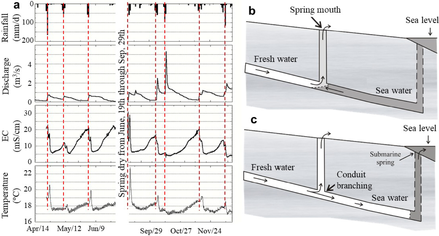
Left, field measurements of rainfall at the recharge area, discharge, electrical conductivity (EC) and temperature of S’Almadrava spring at 8 m.a.s.l in Majorca (Spain) from April, 14th through December, 26th, 1996 year (note that the spring was dry during the summer). Right, conduit branching conceptual model for brackish springs discharging a fraction of seawater above sea level. When the freshwater flow is small (a), the density of mixed water in the vertical branch is smaller than that of seawater and brackish water discharges at the spring mouth. When the freshwater flow is large (b), it intrudes into the conduit connected to the sea, thus creating a submarine spring on the sea floor. Flow is turbulent if all conduits are open (T–T, for Turbulent–Turbulent, model).

The occurrence of a well-developed deep karst system in a seawater intrusion zone appears to be the key factor in the formation of brackish springs. This karst could be formed by the combination of tectonic activity and variations in the sea level over geologic time scales [Fleury et al. 2007]. Moreover, mixing of fresh and seawater may lead to carbonate dissolution [Rezaei et al. 2005], further broadening the conduit section at depth and modifying the seawater intrusion pattern. Under these conditions, a plausible scenario consists of a karst conduit open directly to the sea, allowing mixing at a deep conduit branching [Breznik 1973]. The conduit branching is the junction of three conduits: one from inland with freshwater, another one connected to the sea, and the third one with brackish water leading to the spring mouth (Figure 1b). Such conduit branching has never been directly observed, and the uncertainties associated with its geometry and dimensions have led authors to propose different physical mechanisms to explain salinization at heights above sea level. Proposed salinization mechanisms can be divided into two groups [Stringfield and LeGrand 1969]: salinization due to hydrodynamic effects and salinization due to the greater density of seawater. The first group involves physical conditions of flow in tubular openings or other channels which serve as Venturi tubes. This requires a narrowing of the freshwater conduit at the intersection with the seawater one, allowing the freshwater flowing through to cause a depression, of the order of v²∕2g that sucks in seawater. This mechanism has been proposed for springs showing a rising or steady salinity with increasing discharge flow, such as the Slanac spring (Croatia) [Breznik 1973] and the Makaria spring (Greece) [Maramathas et al. 2006]. However, considering the salinity and elevation of the springs, these situations would require very high groundwater velocities and particular conduit networking morphologies that would be difficult to find in nature or to maintain without erosion, not to mention that mixing fresh and seawater leads to aggressive conditions [i.e., limestone dissolution, Sanford and Konikov 1989; Rezaei et al. 2005; Sanz et al. 2011]. The Venturi effect was also conjectured by McCullough and Land [1992] to explain the inflow of seawater into submarine karst conduits in response to tides and waves. However, the inflow is not in phase with sea level fluctuations, which makes the Venturi effect unlikely. Instead, a hydromechanical effect [Guarracino et al. 2012] explains why the maximum flow rate coincides with the mid-point of the rising tide.

The second group of proposed mechanisms assumes that seawater is sucked at the conduit branching when the hydrostatic pressure in the upwards brackish water conduit is less than that in the seawater tube (that is, when the weight of the brackish mixture up to the spring mouth is less than the weight of seawater up to the sea level). This situation becomes possible if the depth of the branching point is large enough to balance the elevation of the spring mouth with the reduced density of brackish water as compared to seawater. The required depth of the branching point is of several hundred meters, which adds mystery to these peculiar springs. Bakalowicz [2014] attributes deep karst conduits to the Messinian salinity crisis some 5.6 million years ago, when the Mediterranean Sea became isolated from the Atlantic Ocean. This caused the sea-level to drop by at least 1500 m [Ryan 1976], thus lowering the base discharge level and the elevation of karst outlets at large depths below current sea level. In fact, not only the low base level, but also the increased salinity contribute to the development of deep karst conduits. Furthermore, as discussed above, mixing of fresh and salt water leads to calcite subsaturation even when both end members are in equilibrium with calcite and the effect increases with the salinity contrast. Enhanced dissolution coupled to the large drops in sea level elevation during the Messinian salinity crisis may explain why these springs are well documented in Mediterranean shores, but rare elsewhere. Kohout [1965, in Kohout et al. 1977] describe saline springs in Florida. Their observations have been attributed to a thermal convection effect (labelled “Kohout effect”): cold (i.e., dense) seawater enters the aquifer, where it warms up, thus becoming lighter, so that it can rise to a significant height. The relevance of this effect increases with the temperature contrast between the cold and hot waters and with the depth of the cold sea. Both factors are large in Florida [Hughes et al. 2007], but relatively small in the Mediterranean Sea, where we have estimated that the Kohout effect could account for only some 25 cm rise above sea level.

A singular feature of Mediterranean brackish springs is the variation salinity with spring discharge, which has been attributed to variations of freshwater pressure with changes in freshwater flow from the aquifer [Gjurasin 1943, and Kuscer 1950, in Breznik 1973]. This mechanism has been widely accepted for springs that display an inverse relation of flow discharge with respect to salinity, i.e., discharging freshwater during high flows and, below a certain flow-limiting value, increasingly saline waters with decreasing discharge. Examples include Almyros of Heraklion spring (Crete, Greece) [Breznik 1973] Blaz spring (Croatia) [Bonacci and Roje-Bonacci 1997], Pantan [Breznik 1973] and S’Almadrava spring [Sanz et al. 2003].

In some cases, geological constraints suggest that seawater contamination of freshwater flowing through a karst conduit would not be necessarily related to a conduit network connected directly to the sea, but rather to a diffusive seawater intrusion from the porous matrix surrounding the conduit [Arfib and de Marsily 2004]. This situation may occur when a freshwater conduit crosses a saline-intruded fissured matrix zone. Arfib and Ganoulis [2004] performed laboratory experiments demonstrating that a considerable mass exchange may happen under these conditions. Vertical conduits, such as the spring conduit in Figure 1, connected to deep horizontal conduits, such as the fresh and sea water conduits, have been described by Lofi et al. [2012], who link these conduits to karstic activity during the Messinian crisis. While the model of Figure 1 makes geologic sense, it is hard to ascertain whether the sea water conduit is open to the sea or connected through a permeable porous medium. We conjecture that some insight into the most dominant mechanism (open conduit or diffusive connection) in a specific case can be gained from modeling.

There have been attempts to apply numerical models to brackish springs. They have been motivated by the fact that the discharge of those springs represents a precious resource in areas with limited water resources. Modeling proved to be an important tool to test different options of spring development proposed in the last decades [Breznik 1973, 1988; Leontiadis et al. 1988; Bonacci and Roje-Bonacci 1997; Cardoso 1997; Sanz et al. 2003]. Some authors have employed nonlinear analysis or inverse modeling to calculate unit hydrographs and impulse responses from rainfall data in the recharge area [Lambrakis et al. 2000; Pinault et al. 2004]. This type of models, extensively used for freshwater karst springs, use box reservoirs to represent the relationship between an input and an output signal. However, these methods do not consider the physical processes and mechanisms controlling the spring functioning. Maramathas et al. [2003] adopted a different approach based on the mass and energy balance on a hydrodynamic analog, which included three reservoirs flowing from tubes lying adjacent to the spring. Two reservoirs represent the karstic system (two karst subsystems with different depletion period), and the third one emulates the sea. This model assumes the existence of a conduit branching with a conduit open directly to the sea (although this is not simulated), and computes discharge and chloride concentration of the spring using rainfall data as model input. Although the model was successfully applied to the Almyros spring of Heraklion, mixing at the conduit branching and the variable-density turbulent flow in conduits were not considered. In fact, the equations governing variable-density turbulent flow have never been addressed before. We believe that these equations are crucial for a full understanding of the physics of spring functioning. In contrast to this work, Arfib and de Marsily [2004] applied a different conceptual model to the same spring. They assumed the existence of a single freshwater conduit surrounded by a saline porous matrix, where salinization of freshwater in the conduit is a consequence of saline flux from the matrix. This approach considered constant-density turbulent flow in the conduits and mass exchange ratio driven by the head difference between the conduit and the matrix. Surprisingly, these two studies at Almyros spring provided similar results even though they were based on rather different conceptual models and approaches. Therefore, a detailed description of these conceptual models for brackish springs and a direct comparison among them should be addressed.

The objectives of this study are (1) to derive the equations governing density-dependent turbulent flow in open conduits, (2) to describe the salinization mechanisms of inland brackish springs presenting a connection with the sea through an open karst conduit or a diffusive seawater connection, and (3) to compare the spring discharge and concentration response for these two salinization mechanisms.

2. Theory

2.1. Conceptual models of brackish springs

Any conceptual model aimed at explaining brackish springs must include a well developed deep karst system and identify the dominant mechanism of seawater contamination, i.e., the way in which seawater intrudes into the aquifer and mixes with freshwater. Here we analyze two conceptual models that synthesize the features of the most plausible natural systems (Figures 1 and 2). Both conceptual models can explain inverse relations of concentration and discharge of inland springs but apply different salinization mechanisms. The first conceptual model, Turbulent–Turbulent (T–T), assumes that groundwater flows only through a network of conduits and that the seawater contamination occurs at a deep branching point through a conduit of undefined shape connected to the sea (Figure 1). In this environment, ground water follows the hydraulic laws for pipes, resulting on laminar or turbulent flow depending on the velocity and properties of the fluid, and the shape and extent of the conduit section [Chadwick and Morfett 1998]. This problem can be simplified into a mass and energy balance at the conduit branching. Mixing of fresh and saltwater occurs when the interface is placed at the conduit branching (Figure 1a). If the freshwater flow is high enough, freshwater will intrude the seawards conduit and create a submarine spring of, eventually, freshwater (Figure 1b). By contrast, if freshwater flow is very low (or eventually zero), seawater will intrude into the freshwater conduit thus increasing the seawater contamination in the aquifer.

Figure 2.
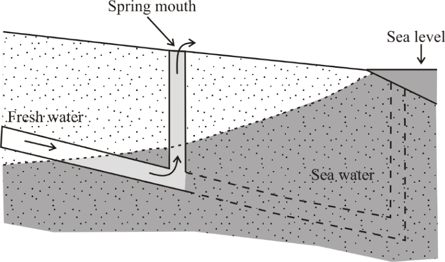
Scheme of the Turbulent–Porous (T–P) conceptual model for brackish springs that considers salinization from seawater by diffuse exchange between the conduit and the surrounding porous matrix. Dotted areas represent the porous/fissured matrix. Water salinity in the conduit and the matrix increases from white to dark grey.

The second conceptual model for spring salinization, which we term Turbulent–Porous (T–P), is a simplification of the model described by Arfib and de Marsily [2004]. They assumed that the freshwater conduit is embedded in a fissured matrix intruded by seawater. For the sake of simplicity, we treat this fissured matrix as a conduit where water flows according to Darcy’s Law (Figure 2).

Given the complexity of karst systems, the schemes of Figures 1 and 2 should be viewed as modeling simplifications. Combinations of multiple branching points contaminated at different depths are likely to occur in natural systems. Nevertheless, the simplicity of these two models should facilitate understanding of the physics controlling the phenomenon, which is the aim of our work.

2.2. Governing equations

The conceptual models considered in this study consist both of a mixing place (i.e., conduit branching) in which a conduit connected to the sea and another conduit from the aquifer inland, join a third vertical conduit with mixed water leading to the spring mouth. Depending on the conceptual model, the seawater conduit is assumed to be an open conduit (T–T case, Figure 1) or a porous/fissured medium (T–P case, Figure 2). In both cases flow is governed by mass and either momentum or energy conservation. We have found no equations for variable density pipe flow in the literature. Therefore we derived them below.

We consider a conduit with open area A(l) (A = A′𝜙, where A′ is the total area and 𝜙 porosity, in the case of a porous medium), where l is the length along the conduit axis. Fluid mass conservation is expressed as:

\frac{\partial 𝜌 A}{\partial t} = - \frac{\partial 𝜌 A v}{\partial l}

(1)

where 𝜌(l,t) is density and v(l,t) is velocity.

Momentum conservation can be expressed in lagrangian coordinates, in which case it expresses Newton’s second law, or in eulerian coordinates. We adopt the second option, which implies that the variation of momentum (∂𝜌Av∕∂t) is equal to the inflow minus outflow of momentum per unit length of conduit ( − ∂𝜌Av²∕∂l) plus the forces acting on the fluid (pressure, weight, and conduit resistance), which, expressed per unit length equals − ∂PA∕∂l −𝜌 Ag cos𝜃−f_p, where cos𝜃 = ∂z∕∂l, z is elevation, and f_p represents the component along l of the forces exerted by the conduit walls over the fluid. That is,

\frac{\partial 𝜌 A v}{\partial t} = - \frac{\partial 𝜌 A v^{2}}{\partial l} - \frac{\partial P A}{\partial l} - 𝜌 A g cos 𝜃 - f_{p} .

(2)

This equation can be used, together with Equation (1), for solving the problem. It can also be written in terms of energy conservation, which may be more intuitive. To this end, we expand the time derivative in Equation (2), use Equation (1) to eliminate the resulting ∂𝜌A∕∂t and perform some minor algebraic manipulations to obtain

𝜌 A \frac{\partial v}{\partial t} = - (𝜌 A \frac{\partial v^{2} ∕ 2}{\partial l} + \frac{\partial P A}{\partial l} + 𝜌 A g cos 𝜃 + f_{p}) .

(3)

Multiplying Equation (3) by v and adding Equation (1) multiplied by v²∕2, yields the energy conservation equation for variable density flow in a pipe:

\frac{\partial 𝜌 A v^{2} ∕ 2}{\partial t} + \frac{\partial 𝜌 A v^{3} ∕ 2}{\partial l} + v \frac{\partial P A}{\partial l} + 𝜌 A v g cos 𝜃 + f_{p} v = 0 .

(4)

This equation expresses energy conservation explicitly, but it is still not easy to apply because of the pressure forces exerted by the conduit walls. The normal component of these cancels if A is assumed constant. Moreover, measurements are rarely more frequent than hourly so that pressure waves can be ignored and the fluid assumed to be incompressible. Therefore, the flow rate (Q = Av) is constant along the conduit. With these simplifications, Equation (4) becomes

- \frac{1}{Q} \frac{\partial 𝜌 A v^{2} ∕ 2}{\partial t} = \frac{\partial}{\partial l} (𝜌 \frac{v^{2}}{2} + P + 𝜌 g z) + \frac{f_{p}}{A} .

(5)

Equation (5) resembles Bernouilli’s equation except for the fact that 𝜌 varies in space and time in response to variations in the proportion of seawater. As a result, 𝜌 cannot be factored out and energy conservation cannot be written in terms of head (energy per unit weight of fluid), but in terms of energy per unit volume. This can be viewed as e =𝜌 gh. Another difficulty is that e is no longer a potential. That is, flow is no longer given solely by differences in local e, but it depends also on the values of 𝜌 along the path. To illustrate this result, assume steady-state and integrate Equation (5) along the conduit, between points 1 and 2, which yields:

(𝜌_{2} - 𝜌_{1}) \frac{v^{2}}{2} + P_{2} - P_{1} + \bar{𝜌} g (z_{2} - z_{1}) + \frac{\bar{f_{p}} L}{A} = 0

(6)

where the overbar stands for spatial average and L is the conduit length

\bar{𝜌}

is not the average along the conduit length, but along the vertical direction:

\bar{𝜌} = \int 𝜌 d z ∕ (z_{2} - z_{1})

. If 𝜌 is constant, then Equation (6) is the traditional expression of energy conservation (e₂ equals e₁ minus dissipated energy). But the fact that e depends on the average density along the (vertical component of the) path hinders its use as state variable. Instead, we will use H =𝜌 v²∕2 + P (energy per unit volume relative to the point elevation) as state variable. Note that, if density is constant, then the traditional Bernouilli head would be h = e∕𝜌g = z + H∕𝜌g.

The expression of $\bar{f_{p}}$ depends on whether the conduit is open (turbulent flow) or porous (Darcy flow). In the case of the open conduit, we have used Manning’s equation:

\frac{\bar{f_{p}}}{A} = \frac{n^{2} \bar{𝜌} g v^{2}}{R_{H}^{4 ∕ 3}}

(7)

where n is Manning’s coefficient and R_H is the hydraulic radius of the conduit (ratio of A to wet perimeter). We have assumed constant cross-sectional area A (and also n). If variable, we would have had to integrate Equation (6), which usually leads, in constant density practice, to an increased

\bar{f_{p}}

, still proportional to Q². In the case of porous medium, Newton’s Law of viscosity suggest that the shear stress will be proportional to velocity:

\bar{f_{p}} = \frac{A 𝜇 v}{k}

(8)

where 𝜇 is viscosity (assumed constant and equal to 1 × 10⁻³ m⋅s/kg) and k intrinsic permeability. This, together with neglecting v² (of the order of 𝜇Pa for normal groundwater velocities), yields Darcy’s law:

v = \frac{k}{𝜇} (\frac{P_{1} - P_{2}}{L} + \frac{\bar{𝜌} g (z_{1} - z_{2})}{L}) .

(9)

The fact that 𝜌 varies in space and time forces us to solve the salt mass conservation equation, which we have written (neglecting dispersion) as:

\frac{\partial c}{\partial t} = - v \frac{\partial c}{\partial l}

(10)

where c is salt mass fraction. Density depends on concentration as:

𝜌 = 𝜌_{f} exp (𝛼 (c - c_{f}))

(11)

where 𝜌_f is the density of fresh water (1000 kg/m³) and 𝛼 equals 0.69167 for mixtures of fresh and seawater (c_s = 3.57 × 10⁻²). It should be noted that having assumed the area to be constant and the fluid to be incompressible, the fluid mass conservation is equivalent to solute mass conservation. This can be easily checked by plugging Equation (11) into Equation (1), which leads to Equation (10).

Solution of these equations requires specifying boundary conditions and continuity at inner nodes (branching point). Pressure is specified as equal to atmospheric pressure (zero relative pressure) at the spring mouth. Energy (per unit volume), $H_{s} = 𝜌_{s} v_{s}^{2} ∕ 2 + P_{s}$ , is specified at the seawater entry point, which can be derived from

𝜌_{s} g e_{s} = 𝜌_{s} g z_{s} + \frac{𝜌_{s} v_{s}^{2}}{2} + P_{s} = 0

(12)

where the subscript s stands for seawater entry point (see Figure 3 for symbols). Continuity at the branching conduit is established in terms of fluid mass, solute mass and energy. That is

\begin{matrix} Q_{m} 𝜌_{m} = Q_{f} 𝜌_{f} + Q_{s} 𝜌_{s} \end{matrix}

(13)

\begin{matrix} Q_{m} 𝜌_{m} c_{m} = Q_{f} 𝜌_{f} c_{f} + Q_{s} 𝜌_{s} c_{s} \end{matrix}

(14)

and

H_{B m} = H_{B s}

(15)

where subscripts f, s and m stand for fresh, sea and mixed waters, respectively, H_Bm is the energy at the branching point obtained from the mixed water conduit, and H_Bs is that obtained from the seawater conduit. These result from result from Equation (6), which yields:

\begin{matrix} H_{B m} & = & P_{B m} + 𝜌_{B m} \frac{v_{m}^{2}}{2} \\ = & \bar{𝜌} g L_{m} (1 + \frac{n_{m}^{2} v_{m}^{2}}{R_{H m}^{4 ∕ 3}}) + 𝜌_{m - spring} \frac{v_{m}^{2}}{2} \end{matrix}

(16a)

where we have assumed that the conduit is vertical L_m = z_spring − z_B. In the steady state case,

\bar{𝜌} = 𝜌_{m - spring} = 𝜌_{m}

, so that H_Bm simplifies to:

H_{B m} = 𝜌_{m} g (L_{m} + b_{m} Q_{m}^{2})

(16b)

with

b_{m} = (1 + 2 L_{m} n_{m}^{2} ∕ R_{H m}^{4 ∕ 3}) ∕ 2 A_{m}^{2}

. Similarly, applying now Equation (6) between the sea entry and the branching points (assuming directly for simplicity that the seawater branch is filled with seawater), yields

H_{B s} = P_{B s} + 𝜌_{s} \frac{v_{s}^{2}}{2} = 𝜌_{s} g (- z_{B} - a_{s} Q_{s}^{2})

(17)

with

a_{s} = L_{s} n_{s}^{2} ∕ R_{H s}^{4 ∕ 3} A_{s}^{2}

. For Darcy flow, H_Bs becomes

H_{B s} = P_{B s} + 𝜌_{s} \frac{v_{s}^{2}}{2} = 𝜌_{s} g (- z_{B} - \frac{𝜇 Q_{s}}{k A_{s}}) .

(18)

In analysing these equations, note that z_B is negative.

Figure 3.
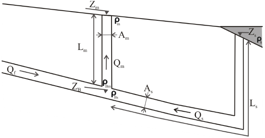
Scheme of the conceptual model for brackish springs including the definition of symbols and notations used in the text. See also Nomenclature list.

3. Methods

3.1. TURBOCODE solver

The above equations are solved using an iterative algorithm (called TURBOCODE) programmed in FORTRAN. Basically, input data include the description of the system (elevation, area, etc.) and the freshwater flow rate. Output consists of the seawater flow rate, Q_s, and derived variables such as mixed water flow rate and concentration (Q_m amd C_m, respectively). The procedure is as follows:

Initialization. Read Q_f(t), z_spring, z_s, z_B, L_m, L_s, n_s (or k_s), n_m (or k_m), A_s, A_m. Time loop. For each time step perform the following operations.
Assume initial value for Q_s [Q_s(t) = Q_s(t − 1); Q_s(0) = Q_f(0)].
Using Q_f and Equations (13), (14) and (11) obtain Q_m, c_m and 𝜌_m, respectively.
Solve transport using Equation (10) by means of a particle tracking method. Once the spatial distribution of concentrations is known, compute $\bar{𝜌}$ . Repeat for the seawater and mixed water conduits.
Compute H_Bm and H_Bs using Equations (16) and (17), or Equation (18).
If H_Bm ≈ H_Bs, go to next time step. If H_Bm > H_Bs, reduce Q_s (otherwise, increase Q_s), and go to step 3.

3.2. Model setting

Simulations are first performed under steady-flow conditions of constant input freshwater flow to facilitate the understanding of the physics of the problem without memory effects. Transient simulations with a time-dependent freshwater input flow are used later to reproduce the actual functioning of brackish springs. The parameter values used in the simulations are listed in Table 1. They do not respond to any particular brackish spring but are selected partly from S’Almadrava spring (Mallorca, Spain) and partially from literature values of other springs of this type. The elevation of the spring mouth is +8 m.a.s.l. for all the simulations.

	Steady-flow	Steady-flow	Transient
	T–P model	T–T model	T–T model
k_s (m²)	10⁻⁶	-	-
L_s (m)	2200	2200	2200
A_s (m²)	35	0.5	0.5
n_s (m^−1∕3⋅s⁻¹)	-	1.5 × 10⁻²	1.5 × 10⁻²
z_s (m)	-	-	700
z_B (m)	540	540	540
A_m (m²)	2	2	2
n_m (m^−1∕3⋅s⁻¹)	1.5 × 10⁻²	1.5 × 10⁻²	1.5 × 10⁻²

See text or Nomenclature list for definition of parameter symbols.

4. Results and discussion

4.1. An energy balance analysis of Freshwater-Seawater mixing at the conduit branching

For a given freshwater flow rate entering the conduit branching, mixing can be viewed as resulting from a mass and energy (or momentum) balance problem. To understand this balance we first calculate the energy at the conduit branching measured from the seawater side (H_Bs) as a function of seawater flow (Q_s), after losses along the seawater conduit (Equations (17) or (18)). This energy is compared to H_Bm (Equation (16)), energy needed to bring the resulting mixed flow to the spring mouth (that is, the energy at the conduit branching measured from the mixed water side). The problem is solved when both energies become identical (Equation (15)). In fact, this is the way TURBOCODE operates. We consider steady-flow conditions, i.e., a constant density in every conduit, for discussion simplicity.

Results for the T–P conceptual model are shown in Figures 4a and 4b, for two series of small and large Q_f values, respectively. H_Bs decreases linearly with seawater flow rate because energy loss at the seawater conduit obeys Darcy’s law (recall that energy at the sea intake is constant and equal to the hydraulic pressure of seawater). This linear relationship is specific to the seawater conduit and does not depend on how much freshwater is flowing into the system. By contrast, the energy necessary to push a column of mixed water towards the spring mouth, H_Bm, depends on both freshwater (Q_f) and seawater (Q_s) flow rates at the conduit branching. For any given Q_f, this energy increases with Q_s because both friction losses and density of the mixture (and thus the weight of the water column) increase with the mixing ratio. For a low Q_f (e.g., 0.25 m³/s, Figure 4a) energy losses in the conduit are small and the dominant term controlling the overall energy is the weight of the water column (Equation (5)), which decreases with decreasing Q_s (i.e., with the density of the mixture). For slightly larger Q_f (e.g., 1.0 m³/s, Figure 4a) we find that less energy is necessary to push up the same Q_s (Figure 4a). This reflects again the fact that energy is most sensitive to the density of the mixed water in the vertical column, which decreases with an increasing Q_f/Q_s ratio. In fact, H_Bm is virtually insensitive to Q_f for null Q_s. This can be attributed to the fact that, for small Q_f, friction losses in the vertical conduit are also small and the energy required to push the mixed water up depends only on the weight of the water column, which is insensitive to Q_f when Q_s is near zero (Figure 4a).

Figure 4.
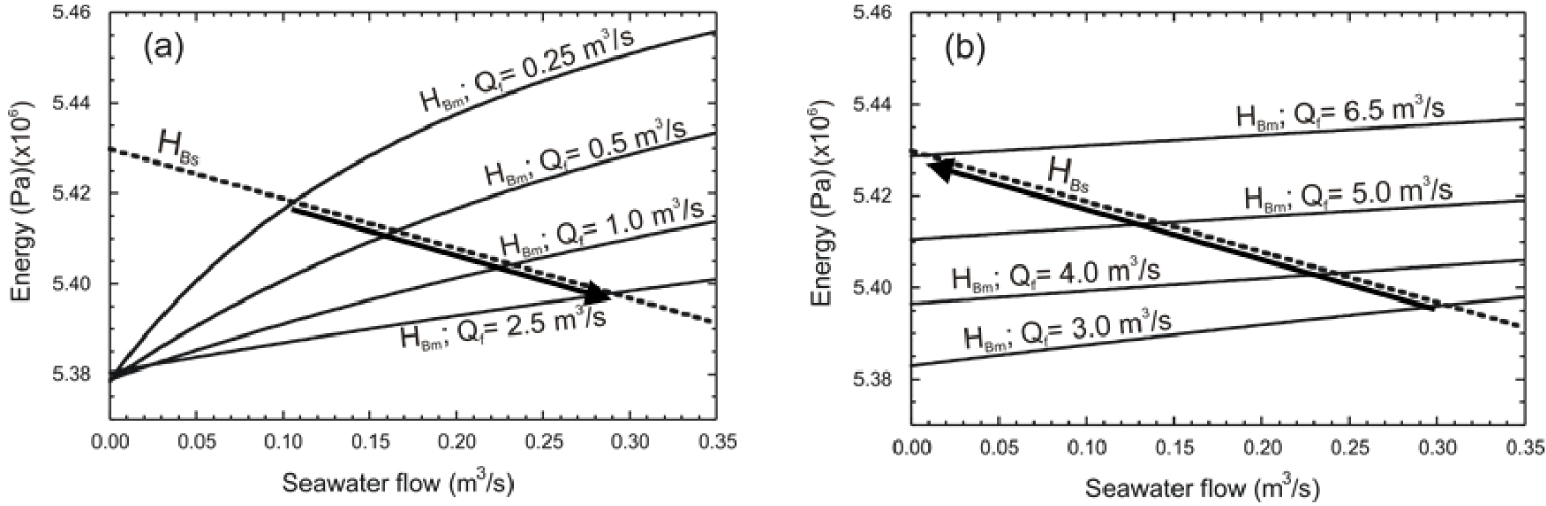
Energy per unit volume computed at the branching point, as seen from the seawater conduit (dotted line, H_Bs) and the mixed water conduit (single line, H_Bm), vs. seawater flow rate for (a) low (0.0–2.5 m³/s) and (b) high (3.0–6.5 m³/s) freshwater flow rates. Results correspond to steady-flow simulations of Turbulent–Porous conceptual model (Table 1).

The situation changes for large values of Q_f (3.0 to 6.5 m³/s, Figure 4b) as the energy loss associated with flow resistance in the upwards conduit become increasingly important. In fact, above a critical Q_f (around 2.5 m³/s for this example) friction losses become more important than density effects. As resistance increases quadratically with the flow rate (Equation (7)), so does the energy required to allow the mixed water to ascend. It should be noted that the increase in energy needed to compensate the resistance of the wall of the conduit is not very sensitive to Q_s because for such high values of Q_f the proportion of Q_s in the total spring discharge is minor.

Every point in which two energy lines (H_Bm and H_Bs) cross in Figure 4 represents a solution of the problem for steady flow regimes, i.e., the energy equilibrium point at the conduit branching for a specific freshwater–seawater mixing ratio (Equation (15)). In summary, for increasing Q_f values, equilibrium occurs with increasing Q_s below the freshwater critical value (Figure 4a), but with decreasing Q_s above it (Figure 4b). The overall trend is represented as a freshwater–seawater curve in Figure 5a. The freshwater–seawater curve is particular for every brackish spring and it is representative of the dimensions of the karst system and the physics of seawater contamination at depth. This critical Q_f value (around 2.5 m³/s for this example, Figure 5a) separates the flow conditions in which the system is primarily controlled either by the weight of the water column or by friction losses. Note that for very large Q_f values (higher than 6.7 m³/s, in this example) the energy equilibrium at the conduit branching is reached for energies higher than the hydraulic pressure of seawater at the conduit outlet to the sea, i.e., for negative Q_s. When this happens, freshwater flows through the conduit branching towards the sea and a submarine spring is created. This situation is addressed in detail in Section 4.3.

Figure 5.
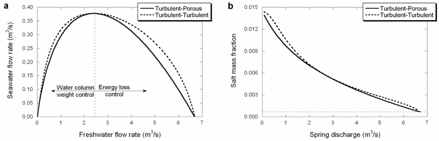
Comparison of simulation results for steady-flow simulations of Turbulent–Turbulent and Turbulent–Porous conceptual models (Table 1). (a) Curves of freshwater–seawater ratio at the conduit branching. The ranges of freshwater flow rate for which the freshwater–seawater ratios are dominated by the weight of the water column or by the energy loss due to resistance are indicated. (b) Relation of salt mass fraction and spring discharge. Horizontal dashed line in the plots on the right marks the pure freshwater salt mass fraction in the simulations.

Figure 5b displays the relationship of salt mass fraction and the spring discharge. The relation reproduces the freshwater–seawater curve discussed above with a decrease on the salinity of the discharge with the flow rate.

For the T–T conceptual model, the behaviour of the mixed water conduit is identical to the T–P case because differences are restricted to the seawater conduit. Still, the T–T case also display two ranges of Q_f depending on whether the solution is controlled by the weight of the mixed water column, or by the energy loss in the conduit (Figure 5a). Differences arise in terms of the energy necessary for a particular seawater flow rate to occur (H_Bs, Equation (17)). The energy loss in the seawater conduit is no longer linear, but quadratic with Q_s, and so does the decrease of H_Bs. As a consequence, the energy equilibrium at the conduit branching is reached for different freshwater–seawater mixing ratios on each conceptual model. Figure 6 illustrates these differences for a low and a high Q_f in our examples (0.25 and 4.5 m³/s). Because the examples chosen to illustrate the two conceptual models are designed to hold the same freshwater–seawater ratio at the Q_f critical value, any equilibrium point for lower or higher freshwater flow rate yields a lower freshwater–seawater ratio at the conduit branching for the T–P conceptual model than for the T–T case (Figure 5a).

Figure 6.
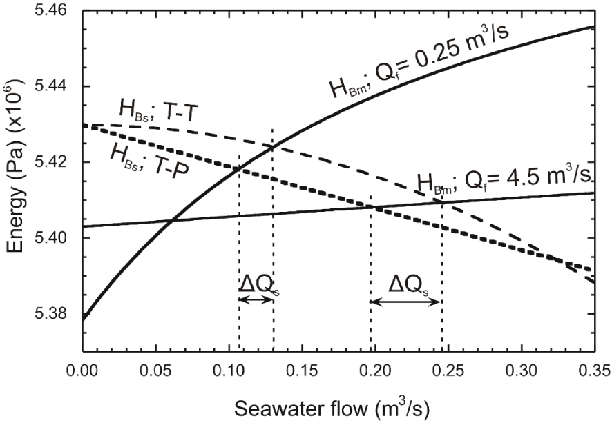
Relationship of energy per unit volume computed at the branching point, as seen from the seawater conduit (H_Bs) and the mixed water conduit (H_Bm) vs. seawater flow rate for 0.25 and 4.5 m³/s of freshwater flow rate. Results correspond to steady-flow simulations of both Turbulent–Porous and Turbulent-turbulent conceptual models (Table 1). Single vertical dashed lines mark the energy equilibrium points. Arrows indicate the difference in seawater flow rate for a particular freshwater flow rate, between the T–T and T–P conceptual models.

The relation of salt mass fraction and spring discharge in the T–T model differs from that obtained for the T–P case near the extreme values of spring discharge (Figure 5b). Thus, the salinity of the spring for lower and higher flow rates on the T–T model increases slightly with respect to that of the T–P case to finally end at the same point. The relationship of the curve at extreme values of spring discharge may therefore be used as a distinctive feature of T–P or T–T conceptual models. This issue is discussed in detail later.

4.2. Solution for the first extreme point (zero seawater and freshwater flow rates)

We discuss here the two points with zero seawater flow in the freshwater–seawater curve. Figure 5a shows that Q_s tends to zero when Q_f approaches zero and for a particular high value of Q_f. Figure 5a shows that when the freshwater inflow from the aquifer decreases to zero, the seawater intrusion at the conduit branching also decreases but in a lesser degree. As a consequence, the density of the mixed water flowing up towards the spring mouth increases as does the weight of the water column connected to the spring mouth. Eventually, energy loss and kinetic terms become negligible. Ignoring all velocity dependent terms in Equations (16) and (17) or (18) yields

𝜌_{m} L_{m} = - 𝜌_{s} z_{B}

(19)

which simply expresses that the weight (pressure) of seawater at the branching point equals the weight of the mixed water column. This expression allows us to derive the elevation of the branching point from the elevation of the spring mouth and the concentration for extremely low flow. In fact, using Equation (11) for 𝜌_m and 𝜌_s, and L_m = z_spring − z_B yields

z_{B} = \frac{z_{spring}}{1 - exp [𝛼 (c_{s} - c_{m})]}

(20)

where z_B is negative because c_m < c_s. It is also worth pointing that, in the T–T case, all ignored terms depend on Q². Therefore, concentration at the spring mouth should tend to a constant value as Q tends to zero. That is

{\frac{\partial c_{m}}{\partial Q}|}_{Q = 0} = 0

(21)

which explains why c_m becomes constant for small Q in the T–T graph of Figure 5b.

On the contrary, for the T–P case the concentration at the spring mouth decreases linearly with Q for small Q values (Figure 5b). In fact, equating H_Bm (Equation (16)) and H_Bs (Equation (18)) and taking derivatives yields

{\frac{\partial c_{m}}{\partial Q}|}_{Q = 0} = - \frac{𝜇}{L_{m} A_{s} k} \frac{(c_{s} - c_{f})}{𝛼 (c_{m} - c_{f})}

(22)

which suggests that hydraulic resistance of porous conduit could be derived from the slope of the c_m vs. Q graph.

That the behaviour near the origin does not depend much on hydraulic parameters is also shown in the freshwater vs. saltwater discharge curve. Taking derivatives of the mass balance equations (13) and (14) with respect to the Q_f yields

{\frac{\partial Q_{s}}{\partial Q_{f}}|}_{Q_{f} = 0} = \frac{𝜌_{f} c_{m}}{𝜌_{s} (c_{s} - c_{m})}

(23)

which depends solely on c_m. Since c_m at the origin only depends on Z_B, so does the slope of the Q_s–Q_f curve. This can indeed be seen in Figure 5a. In fact, this slope defines a straight line above which it is not possible to find any valid Q_s value.

In summary, the behaviour of the Q_s–Q_f and c_m–Q curves at the origin is informative of the depth of the branching point, which can be derived either from c_m or from the slope of the Q_s–Q_f curve. It is also informative of the type of seawater conduit: turbulent if the slope of the c_m–Q curve is zero, or darcian, otherwise. In the latter case, the slope of the c_m–Q curve at the origin allows one to derive the hydraulic resistance of the seawater conduit.

For our example, representing a brackish spring with a spring mouth at +8 m.a.s.l. and a conduit branching at −540 m.a.s.l. (Table 1), we obtain a maximum potential salt mass fraction at the spring mouth of 1.4 × 10⁻² (equivalent to 38% of seawater) (Equation (20)). The grey area in Figure 7 illustrates all freshwater–seawater combinations representing a salt mass fraction over the maximum potential calculated, i.e., combinations out of the calculated potential range. In other words, it shows freshwater–seawater mixing ratios that would never be measured at the spring discharge of our modeled brackish spring. As expected, for either conceptual model considered, the solution fits the maximum potential freshwater–seawater ratio for very low Q_f values. As the Q_f increases the solution separates from that potential ratio given that the energy loss becomes more significant. It should be pointed out that the dependence of Q_s on Q_f is more linear in the T–T case than in the T–P case. This is attributed to the fact that H_Bs remains essentially constant for low Q_s (Figure 6). This implies that salinity at the spring mouth will tend to be constant value for a range of very low flow rates (say, below 0.2 m³/s in our example) in the T–T case, while it will grow steadily to the same value in the T–P case. It relevant to point out that this quasi linear behaviour does not require a Venturi effect, as suggested by Maramathas et al. [2006] for the Makaria spring.

Figure 7.
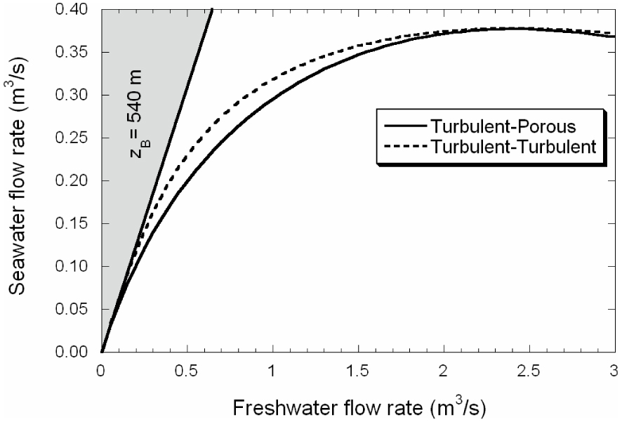
Curve of freshwater–seawater ratio at the conduit branching for steady-flow simulations of Turbulent–Turbulent and Turbulent–Porous conceptual models (Table 1). The grey area mark freshwater–seawater ratios out of the potential range for the spring mouth elevation and conduit branching depth of the brackish spring simulated.

4.3. Second extreme point (Q_s = 0,Q_f > 0) and submarine freshwater spring

The second situation in which we have zero Q_s occurs for a particular high value of Q_f (6.7 m³/s in our example, Figure 5a). As discussed before, the energy loss at the mixed conduit increases quadratically with the mixed water flow, so that the seawater flow reduces to minimize the concentration of the mixed water, and therefore the weight of the mixed water column. This explanation implies that the resulting flow rate is independent of the seawater conduit behaviour. In fact, using again the energy continuity condition (Equation (15) with (16b) for H_Bm and either (17) or (18) for H_Bs) together with Q_s = 0, yields

Q_{f} = \sqrt[2]{\frac{- 𝜌_{s} z_{B} - 𝜌_{f} L_{m}}{𝜌_{f} b_{m}}} .

(24)

Simple inspection of this equation shows that Q_f at this point solely depends of the elevation of spring and branching point and turbulent losses in the mixed conduit. Energy continuity, together with fluid and solute mass conservation can be used to compute the derivatives of C_m with respect to Q_m and Q_s with respect to Q_f. The derivation is a bit tedious and the results less informative than at the origin. The only relevant result is that the slope of both curves is far larger in the T–T case, than in the T–P case. This finding is related to the fact that head losses in the seawater conduit are proportional to $Q_{s}^{2}$ in the T–T case, so that they are negligible for small Q_s. They are proportional to Q_s in the T–P case, so that they are sizeable even for small Q_s.

For even higher Q_f, the functioning of the spring is inverted. The energy necessary at the conduit branching to exceed the energy loss in the mixed water conduit is too high to be maintained. As a consequence, freshwater starts to flow towards the sea reducing the mixed water flow upwards. The freshwater intruding into the conduit connected to the sea promotes a negative Q_s (i.e., towards the sea) and a submarine spring is created. Concentration at the spring mouth becomes pure freshwater while the concentration in the submarine spring mouth is initially that of pure seawater. When that happens the functioning of the system changes radically and becomes dependent on the magnitude of the freshwater intrusion into the conduit connected to the sea. In fact, the magnitude of the freshwater intrusion will determine the salinity of the submarine spring, which may even become pure freshwater in an extreme situation. It is important to note that the minimum Q_f value for which a negative Q_s is produced is essential for a complete characterization of the spring functioning since it defines the flow ranges for which the system behaves as an inland or a submarine spring. It is also important to note that although any freshwater–seawater curve calculated for a particular brackish spring has a theoretical Q_f before the Q_s is inverted, the actual chances for that high Q_f to occur in the aquifer may be very low and that situation could never happen in reality. Measuring pure freshwater at the spring mouth during high flow discharge periods may be an indicator that freshwater is intruding into the seawater conduit thus forming a submarine spring.

To obtain a more realistic solution to the problem involving submarine springs, equations must be solved in transient-flow mode. In order to do that, a time-dependent freshwater inflow function is designed with an increase from 5.0 to 9.0 m³/s followed by a decrease back to 5.0 m³/s, with a variation rate of 0.5 m³/s every 24 h. This freshwater function is introduced in a T–T simulation type with a sea opening at −700 m.a.s.l. (Table 1). Note that for the T–T conceptual model the depth of the sea outlet needs to be defined (Equation (17)), since the average density in the conduit connecting with the sea may no longer be equal to that of the seawater. Results are shown in Figure 8.

Figure 8.
Curve of freshwater–seawater ratio at the conduit branching for transient simulation of Turbulent–Turbulent conceptual model (Table 1). Arrows indicate the order at which the values are generated when increasing freshwater flow rates (filled arrows) and when decreasing freshwater flow rates (simple arrows). The negative seawater flow situation applies briefly while there is seawater within the seawater conduit.

Under these flow circumstances, the controlling parameters are the depth of the sea outlet and the average density in the conduit connected to the sea (which depends on the length of this conduit and the magnitude of the freshwater intrusion into this conduit). If the depth of the sea outlet is equal or less than that of the conduit branching, the pressure at the sea outlet is therefore less than that at the conduit branching, and freshwater is able to easily intrude into the conduit. The submarine discharge will become fresh very quickly, only depending on the length of the conduit.

By contrast, if the sea outlet is deeper than the conduit branching (as it happens in our example, Figure 8), the velocity of the freshwater intruding into the seawater conduit will be very small because pressure at the branching point needs to increase to overcome the double effect of having a higher pressure at the sea opening, and the reducing density of the water filling the conduit, initially assumed to be pure seawater. In Figure 8, freshwater flow, Q_f, increases from 6.7 to 8.75 m³/s, with a negligible flow in the seawater conduit. As Q_f increases further, pressure at the branching becomes sufficient to overcome the reduced density of freshwater filling the sea conduit and the submarine spring discharges pure freshwater (freshwater flow above 8.75 m³/s, Figure 8). When Q_f decreases again (e.g., after an important rainfall event) the behavior of the system inverts and the fluid in the conduit becomes positive again (freshwater flow reduction from 8.75 to 6.7 m³/s, Figure 8). Note that for this range of flow rates, although groundwater flows back towards the conduit branching, the mixed water moving upwards to the spring is still pure freshwater. Only when the seawater front reaches the conduit branching (at 6.7 m³/s approx., in our example) will the spring discharge become salinized again.

4.4. Sensitivity analysis

A set of simulations are conducted to illustrate the sensitivity of the spring response with respect to the parameters used in the simulation. First of all, we identify the controlling parameters for each conceptual model on steady-flow conditions from Equations (16) and (17) or (18). Then a perturbation of ±20% is applied separately over the base value of every parameter in order to quantify the relative sensitivity of the solution to that parameter (see parameter unperturbed base values in Table 2). The analysis is performed over steady-flow simulations since it allows a better isolation of the effect that each parameter has on the solution. The sensitivity analysis is discussed separately for the two conceptual models. Results are presented in terms of freshwater–seawater curves and relation of salt mass fraction with spring discharge. These representations are especially useful because they can be compared with the most commonly available field measurements in brackish springs, which are spring flow rates and water concentration with time.

T–P model		T–T model
Parameter	Value	Parameter	Value
A_m (m²)	2.0	A_m (m²)	2.0
n_m	1.5 × 10⁻²	n_m	1.5 × 10⁻²
z_B (m)	540.0	z_B (m)	540.0
L_s∕k_s A_s (m⁻³)	6.3 × 10⁺⁷	$n_{s} \sqrt{L_{s}} ∕ A_{s}$ (m^−2.5)	1.41

See text or Nomenclature list for definition of parameter symbols.

4.4.1. Turbulent–Porous conceptual model

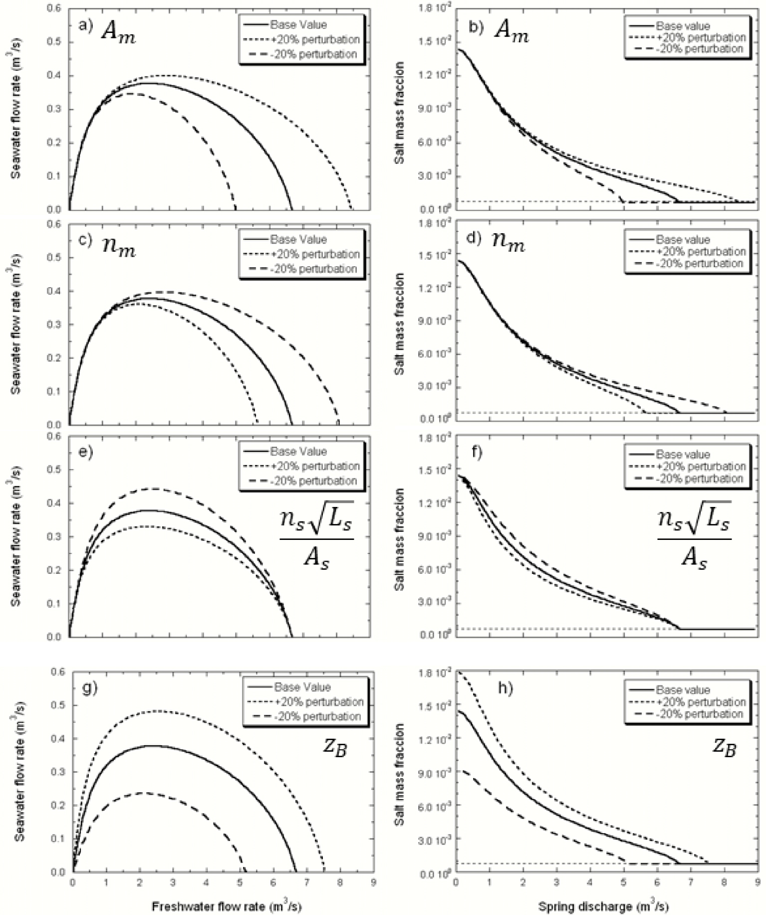
The solution for a T–P problem depends only on four parameters: A_m, n_m, L_s∕k_s A_s and Z_B. Although this analysis is performed for steady-flow conditions, these four parameters (plus the history of Q_f(t)) would control a transient-flow simulation as well. Figure 9 displays the results (Q_s vs. Q_f, and c_m vs. Q_m) for the base case and perturbated parameters.

Figure 9.
Sensitivity analysis Q_s vs. Q_f curve (left column) and c_m vs. Q_m (right column), with respect to every controlling parameter of the Turbulent–Porous conceptual model (T–P): A_m (cross sectional area of the mixed water conduit), n_m (Manning’s coefficient of the mixed water conduit), L_s∕k_s A_s (ratio of length, permeability and cross section area, of the seawater conduit) and z_B (depth of the branching point). The horizontal dashed line in the plots on the right marks the pure freshwater salt mass fraction in the simulations.

The parameters A_m and n_m control the resistance of the vertical conduit to the water flow (Equation (16)) and therefore show a similar—but opposite-influence on the spring response (Figure 9a–d). As the energy loss in the vertical conduit is a quadratic function of the water flow, the effect of these parameters is negligible for low Q_f or spring discharges (recall that for low Q_f the solution was primarily dominated by the weight of the water column, Figure 5a). However, their influence rapidly increases with Q_f (Figure 9a,c). As a consequence, the expected spring concentration will increase with decreasing flow resistance, although this effect can be observed only for high spring discharges (Figure 9b,d). A_m not only controls the energy loss but also the velocity of the groundwater in the conduit, and therefore for transient-flow situations presents a relatively stronger influence on the spring response than n_m.

The solutions display a negative sensitivity with respect to the parameter L_s∕k_s A_s (Figure 9e,f), i.e., an increase in the resistance to flow in the seawater conduit reduces the proportion of seawater entering the conduit branching. Obviously, the solution does not change near the two zero-Q_s situations, which is also consistent with the equations governing the functioning mechanism of the spring. As discussed above, when Q_f approaches zero, the solution only depends on the depth of the conduit branching (Equation (18)) and, accordingly, the solution shows no sensitivity to any other parameter than z_B (Figure 9g,h). Further, for L_s∕k_s A_s the solution shows no sensitivity at the other zero-Q_s point either because the energy equilibrium for this situation to occur depends on the depth of the conduit branching and on the resistance in the vertical conduit (Figure 9, Equations (16) and (18)).

Finally, the depth of the conduit branching, z_B, exerts an influence on the spring concentration for any discharge (Figure 9h). As discussed above, the proportion of seawater entering the conduit branching increases with z_B because the pressure resulting from the weight of the seawater column increases accordingly (Figure 9g). Consequently, the spring salt mass fraction for any spring discharge is higher for deeper conduit branchings (Figure 9h). This parameter influences the energy curves of both the seawater and the mixed water conduit (Equations (16) and (18)). The slope of the freshwater–seawater curve when the freshwater flow approaches zero, is also dependent on the parameter value (recall Equation (19), Figure 9g). Results also show that shallow conduit branchings will facilicitate the formation of submarine springs because the minimum Q_f necessary to inverse Q_s is smaller.

An overall analysis of Figure 9 suggests that a spring with measures in a broad range of discharges may allow us to characterize: (1) the resistance of the upwards conduit (but not n_m and A_m L_m separately) from the response at high flow rate; (2) the depth of the branching point (z_B) from the concentration at low discharges; and (3) the hydraulic resistance of the seawater conduit from the slope of c_m vs. Q_m at low spring discharges.

4.4.2. Turbulent–Turbulent conceptual model

The solution for a T–T problem depends on four parameters: A_m, n_m, $n_{s} \sqrt{L_{s}} ∕ A_{s}$ and Z_B. Figure 10 shows the results of the sensitivity of the solution to these parameters. Results for this case are generally analogous to those of the T–P case and similar discussion could be applied. The most striking feature is that the behaviour at the two zero Q_s points is virtually insensitive to flow resistance parameters at the seawater conduit. This is consistent with Equations (21) and (24). The main difference with the T–P case is that results are less sensitive to z_B and that the abrupt change in Q_s near the critical Q_f remains nearly vertical for all parameter combinations (reflecting that energy losses in the seawater conduit are proportional to $Q_{s}^{2}$ , so that they drop more significantly to zero when Q_s tend to zero than in the T–P case). The other relevant feature is that, for all parameter sets the maximum Q_s is flatter in the T–T case than in the T–P case.

Figure 10.
Sensitivity analysis Q_s vs. Q_f curve (left column) and c_m vs. Q_m) (right column), with respect to every controlling parameters of the Turbulent–Turbulent conceptual model (T–T): A_m (cross section areal of the mixed water conduit), n_m (Manning’s coefficient of the mixed water conduit), $n_{s} \sqrt{L_{s}} ∕ A_{s}$ (ratio of Manning’s coefficient, length and cross section area, of the seawater conduit) and z_B (depth of the branching point). Horizontal dashed line in the plots on the right marks the pure freshwater salt mass fraction in the simulations.

In summary, the sensitivity analysis confirms that the main features to distinguish the T–T and T–P models are: (1) near the origin: the slope of the c_m vs. Q_m curve (near zero in the T–T case), (2) near the critical Q_f point, the slope of the Q_s vs. Q_f curve (nearly vertical in the T–T case), and (3) near the maximum Q_s point, the flatness of the Q_s vs. Q_f curve (inverted parabola and asymmetric in the T–P case and flatter, nearly circumferential in the T–T case).

4.5. Comparison with field data

The results obtained in TURBOCODE simulations are compared with field data observations from three brackish springs: S’Almadrava spring (Mallorca, Spain, Figure 1), Pantan spring (Croatia) and Almyros of Heraklion spring (Crete, Greece). Figure 11 shows the relationship of the spring concentration vs. discharge for S’Almadrava [Sanz et al. 2002], Pantan [Breznik 1973] and Almyros [Monopolis et al. 1995]. Beyond differences in number of observations and in salinity or discharge ranges, all springs display similar patterns with a decreasing salinity for increasing spring discharges (Figure 11). Based on the data available, the authors proposed that the salinization of these springs is due to the greater density of seawater in the T–T scheme, as discussed below. Field data for S’Almadrava covers a wide range on spring discharges (Figure 11a). From these observations, the conceptual model controling the functioning of S’Almadrava spring would be a T–T case because: (1) the relation of salinity and flow rate is far from linearity for medium spring discharges, (2) for very low discharges, the spring concentration seems to reach a constant value (Figures 5b and 10, right hand side plots), and (3) Q_s remains quite constant near its maximum.

Figure 11.
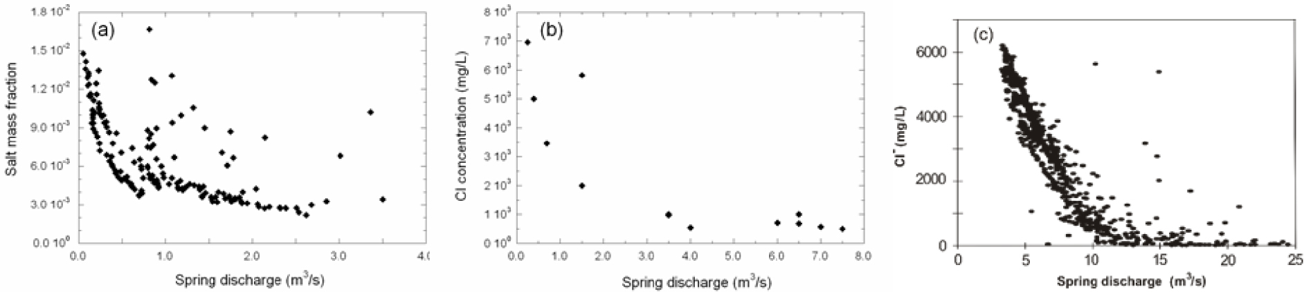
Relationship of spring discharge and water quality for (a) S’Almadrava spring (Mallorca) [after Sanz et al. 2002]; (b) Pantan spring (Croatia) [after Breznik 1973]; and (c) Almyros spring of Heraklion (Crete) [after Monopolis et al. 1995].

The available observations for Pantan spring also cover a wide range of spring discharges and the connection to the sea seems to be controlled by a karst conduit (T–T case) (Figure 11b). However, the limited number of data available prevents further discussion. In contrast, many observations are available for Almyros spring (Figure 11c). Data concentrates for medium to high spring discharges, where the spring clearly discharges freshwater. Field measurements seems to form a curve of high linearity. This observation seems more consistent with a T–P case (Figures 5b and 9, right hand side figures). However, the distinction of the conceptual model of Almyros turns out to be difficult due to the lack of data for very low flow discharges.

The fact that field measurements display some spreading with respect to the simulated curves for steady-flows presented in this study could be attributed to the memory effects resulting from the dynamic nature of the systems or be a consequence of the higher complexity of the karst network in the aquifers (e.g., multiple conduit branchings), compared with the simplifications considered in this study.

The freshwater seawater flow rates plots from field measurements in S’Almadrava spring and Almyros spring [Maramathas et al. 2006] are shown in Figure 12. The data from S’Almadrava spring shows a zero-Q_s point for Q_f approaching zero. The freshwater–seawater ratio then increases linearly with Q_f before gradually stabilizing in about 0.15 m³/s of Q_s for a wide range of Q_f. This pattern agrees with simulations of this study for T–T conceptual model (Figures 5a and 10, left hand side figures). The field data for this spring does not show any significant decrease in Q_s for higher Q_f, and therefore Q_f of at least 4 m³/s are expected to be necessary for the formation of a submarine spring.

Figure 12.
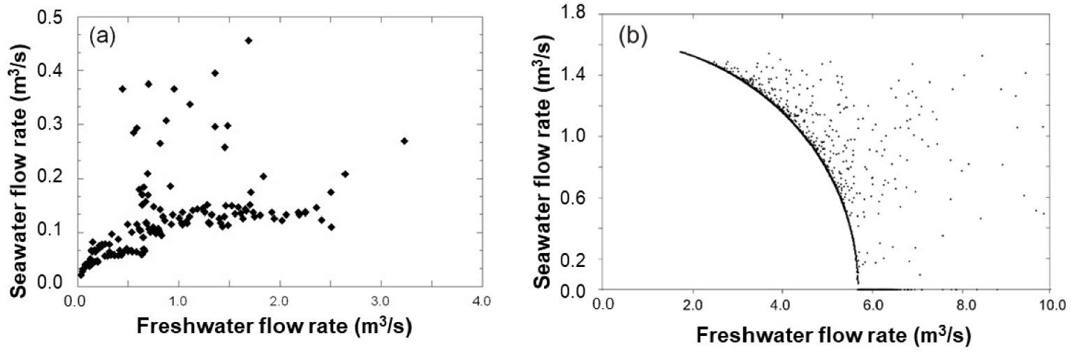
Seawater flow rate vs. freshwater flow rate for (a) S’Almadrava spring (Mallorca, Spain); and (b) Almyros of Heraklion spring (Crete, Greece) [after Maramathas et al. 2006]. Note that the flow rate at Almyros never becomes small enough for the seawater flow rate to drop.

Field measurements for Almyros spring form a curve with an abrupt decrease in Q_s with Q_f until a zero-Q_s point is reached for about 5.6 m³/s Q_f. Null seawater contribution (that is, pure freshwater discharging at the spring) is maintained for higher Q_f values, in line with the formation of a submarine spring at the sea bottom predicted in our simulations (Figure 8). The formation of submarine springs may be reconcilable with either T–T or T–P conceptual models and we would need more geology information to confirm any conceptual model. However, the abruptness of the freshwater–seawater curve when approaching the zero-Q_s point indicates that a T–T scheme is more likely at Almyros spring. The different interpretations that may arise from the available observations for Almyros spring point out the difficulty of selecting the conceptual model governing brackish springs. This is especially so when the available observations do not cover a wide range of spring discharges including the two zero-Q_s points. In fact, Arfib and de Marsily [2004] and Maramathas et al. [2003], built numerical simulations describing the T–P and T–T conceptual models, respectively, and obtained reasonable results in both cases.

5. Conclusions

In this study we use hydraulic models to reproduce the physics controlling the salinization of brackish springs. We derived the equations governing variable-density turbulent flow in conduits and solved them numerically. The solution has been found for systems consisting of a deep mixing place in which a freshwater conduit and another conduit connected to the sea join a third conduit with mixed water leading to the spring mouth. Two conceptual models have been tested: the Turbulent–Turbulent case in which the salinization of the conduit branching comes from a karst conduit connected to the sea, and the Turbulent–Porous case in which the seawater intrusion occurs through a porous/fissured matrix (Figures 1 and 2, respectively). In both cases flow is governed by mass and either momentum or energy conservation. The response of the spring concentration to the variation of freshwater flow rate from the aquifer is evaluated in steady-flow conditions in terms of energy balance at the mixing point and freshwater–seawater ratios. For low freshwater flow rates, the spring response is controlled by the weight of the water column flowing from the conduit branching to the spring mouth. As the freshwater flow rate increases, the energy loss increases accordingly and the resistance of the conduit walls to flow becomes the controlling factor. Results are similar for both conceptual models for medium spring discharges, although the relation of spring salinity and discharge is more linear for the Turbulent–Porous case. Additionally, for the Turbulent–Turbulent case, the spring concentration becomes constant when the spring discharge tends to zero. This points out that in this situation the solution depends only on the water column weight in the vertical conduit. In fact, the spring dries up when the excess in elevation of the spring mouth is balanced by the excess of density of seawater with respect to that of the mixed water in the conduit connected to the spring mouth. Further, the depth of the conduit branching can be then approximated from the elevation of the spring mouth and the spring salinity at very low discharges.

The sensitivity of the spring response with respect to the parameters controlling the system is also evaluated in terms of freshwater–seawater ratios and the relation of spring discharge and salt mass fraction. For the Turbulent–Porous case, the simulation is sensitive to A_m and n_m for high freshwater flow rates, but their effect is opposite: salinity increases for larger A_m and smaller n_m. This is attributed to the quadratic increase of energy loss in the vertical conduit with the spring discharge. The solution for medium freshwater flow rates depends on L_s∕k_s A_s. A higher parameter value increases the energy loss of the seawater intruding into the aquifer and thus reduces the salinitzation at the conduit branching. Finally, for low freshwater flow rates the solution only depends on the depth of the conduit branching since it controls the limiting water column weight that the system can support before the spring dries up. The sensitivity of the solution in the Turbulent–Turbulent case is very similar to that for the Turbulent–Porous one for the parameters A_m, n_m and Z_B. The resistance to flow in the conduit connected to the sea can be expressed now as $n_{s} \sqrt{L_{s}} ∕ A_{s}$ ., where an increase of the resistance not only reduces the proportion of the seawater mixing at the branching point but also the salinity discharging from the spring. This effect is only important for medium freshwater flow rates since the solution for high flow rates is dominated by the energy loss in the vertical conduit rather than in the conduit connected to the sea. If the freshwater flow rate overpasses a limiting value, the high energy loss in the vertical conduit may promote a freshwater intrusion into the conduit connected to the sea. This will generate the formation of a submarine spring in the sea floor of variable density depending on the extent of the intrusion and the depth of the conduit outlet in the sea. This situation may be identified by measuring freshwater concentration during stages of high spring discharges in the spring.

The prediction curves of freshwater–seawater and the relationship of spring discharge and salt mass fraction are compared with field data from S’Almadrava spring, Pantan spring and Almyros of Heraklion spring. The simulation results show a good agreement with the field data available, and provide insights to identify the conceptual model governing every particular spring. The analysis highlights the importance of acquiring high frequency field data encompassing the whole range of spring discharges for a sound understanding of the spring functioning, specially at the extreme points of low seawater flow.

The freshwater–seawater curve is specific to every brackish spring and it is representative of the dimensions of the karst system and the salinization mechanism. In the light of our findings, an analysis based on the freshwater–seawater ratios rather than on the relationship of spring concentration and discharge proves to be more suitable for identifying the salinization mechanisms of brackish springs.

Nomenclature

A_l	Cross sectional area of a conduit
A′	Total area of a conduit
𝜑	Porosity
l	Length along the conduit axis
t	Time
𝜌	Water density, defined in Equation (11)
𝜌₀	Density of pure water
v	Velocity
f_P	Shear component of the forces exerted by the conduit walls over the fluid
Q	Water flow rate at conduit
z	Depth
z_spring	Depth at spring mouth
z_s	Depth at the seawater entry point
L	Conduit length
n	Manning’s coefficient
R_H	Hydraulic radius of the conduit (ratio of A to wet perimeter)
𝜇	Viscosity
k	Intrinsic permeability
c	Salt mass fraction
𝛼	Coefficient
H	Energy per unit volume
H_Bf	Energy at the conduit branching measured from the freshwater side
H_Bs	Energy at the conduit branching measured from the seawater side
H_Bm	Energy at the conduit branching measured from the mixed water side
f	Subscript for freshwater and freshwater conduit
s	Subscript for seawater and seawater conduit
m	Subscript for mixed water and mixed water conduit
B	Subscript for conduit branching
$\bar{𝜌}$	Overbar stands for spatial average

Conflicts of interest

Authors have no conflict of interest to declare.

Acknowledgments

Comments by two anonymous reviewers and especially John M. (Jack) Sharp are gratefully acknowledged. Most of this work was funded by the European Union (SALTRANS project, contract no. EVK1-CT-2000-00062) and the Spanish Government (project Medistraes3. grant no. PID2019-110311RB-C21), and IDAEA-CSIC Center of Excellence Severo Ochoa (Grant CEX2018-000794-S). ES is also grateful to a FI doctoral scholarship from the Catalan Government. The authors wish to acknowledge Dr. Guangjing Chen for his help and useful comments on the formulation and code design. Data and documentation related to S’Almadrava spring was gently provided by the Junta d’Aigües de Balears.

Bibliographie

[Acikel and Ekmekci, 2018] S. Acikel; M. Ekmekci Assessment of groundwater quality using multivariate statistical techniques in the Azmak Spring Zone, Mugla, Turkey, Environ. Earth Sci., Volume 77 (2018) no. 22, pp. 1-14 | DOI

[Ackerer et al., 2023] P. Ackerer; J. Carrera; F. Delay Identification of aquifer heterogeneity through inverse methods, C. R. Géosci., Volume 355 (2023) no. S1 (Online first) | DOI

[Arfib and de Marsily, 2004] B. Arfib; G. de Marsily Modeling the salinity of an inland coastal brackish karstic spring with a conduit-matrix model, Water Resour. Res., Volume 40 (2004), pp. 1-10 | DOI

[Arfib and Ganoulis, 2004] B. Arfib; J. Ganoulis Modélisation physique de l’intrusion d’eau de mer dans un aquifère karstique: cas de l’Almyros d’Héraklion (Crète), C. R. Geosci., Volume 336 (2004) no. 11, pp. 999-1016 | DOI

[Arfib et al., 2007] B. Arfib; G. de Marsily; J. Ganoulis Locating the zone of saline intrusion in a coastal karst aquifer using springflow data, Ground Water, Volume 45 (2007), pp. 28-35 | DOI

[Bakalowicz, 2014] M. Bakalowicz Karst at depth below the sea level around the Mediterranean due to the Messinian crisis of salinity. Hydrogeological consequences and issues, Geol. Bel., Volume 17 (2014) no. 1, pp. 96-101

[Bonacci and Roje-Bonacci, 1997] O. Bonacci; T. Roje-Bonacci Sea water intrusion in coastal karst springs: example of the Blaz Spring (Croatia), Hydrol. Sci. J., Volume 42 (1997), pp. 89-100 | DOI

[Breznik, 1973] M. Breznik The origin of brackish karstic springs and their development, Geologija, Volume 16 (1973), pp. 83-186

[Breznik, 1988] M. Breznik Development of the karstic spring Almyros in Greece, Geologija, Volume 31 (1988), pp. 555-576

[Cardoso, 1997] G. Cardoso Comportamiento de los manantiales del karst nororiental de la Serra de Tramuntana, Mallorca, Ph. D. Thesis, Dep. of Civil Eng., UPC, Barcelona (1997)

[Chadwick and Morfett, 1998] A. Chadwick; J. Morfett Hydraulics in Civil and Environmental Engineering, E and FN Spon, New York, 1998 | DOI

[Crosby and Crosby, 1896] F. W. Crosby; W. O. Crosby The sea mills of Cephalonia, Technol. Q., Volume 9 (1896), pp. 6-23

[de Marsily, 1986] G. de Marsily Quantitative Hydrogeology, Paris School of Mines, Fontainebleau, 1986

[de Marsily, 2009] G. de Marsily L’eau, un trésor en partage, Dunod, Paris, 2009

[Fleury et al., 2007a] P. Fleury; M. Bakalowicz; G. de Marsily Submarine springs and coastal karst aquifers: A review, J. Hydrol., Volume 339 (2007), pp. 79-92 | DOI

[Fleury et al., 2007b] P. Fleury; M. Bakalowicz; G. de Marsily; J. M. Cortes Functioning of a coastal karstic system with a submarine outlet, in southern Spain, Hydrogeol. J., Volume 16 (2007) no. 1, pp. 75-85 | DOI

[Fouqué, 1867] F. Fouqué Rapport sur le tremblement de terre de Céphalonie et de Mételin en 1867, Archives des missions scientifiques et littéraires, Volume 4, 1867, pp. 445-482

[Fuller, 1907] M. Fuller Conditions of circulation at the sea mills of Cephalonia, Geol. Soc. Am. Bull., Volume 18 (1907) no. 1, pp. 221-232 | DOI

[Gjurasin, 1943] K. Gjurasin Prilog hidrografiji primorskog krsa, Tech. Vjesn., Volume 60 (1943), pp. 1-17

[Guarracino et al., 2012] L. Guarracino; J. Carrera; E. Vázquez-Suñé Analytical study of hydraulic and mechanical effects on tide-induced head fluctuation in a coastal aquifer system that extends under the sea, J. Hydrol., Volume 450 (2012), pp. 150-158 | DOI

[Hughes et al., 2007] J. D. Hughes; H. L. Vacher; W. E. Sanford Three-dimensional flow in the Florida platform: Theoretical analysis of Kohout convection at its type locality, Geology, Volume 35 (2007) no. 7, pp. 663-666 | DOI

[Kohout et al., 1977] F. A. Kohout; H. R. Henry; J. E. Banks; K. L. Smith; G. M. Griffin Hydrogeology related to geothermal conditions of the Floridan Plateau, The Geothermal Nature of the Floridan Plateau (D. L. Smith; G. M. Griffin, eds.), Volume 21, Bureau of Geology, Div. of Resour. Manag., Tallahassee, FL, 1977, pp. 1-41

[Kohout, 1965] F. A. Kohout A hypothesis concerning cyclic flow of salt water related to geothermal heating in the Floridan aquifer, Trans. N. Y. Acad. Sci., Volume 28 (1965) no. 2, pp. 249-271 | DOI

[Kuscer, 1950] I. Kuscer Kraski izviri ob morski obali, Razprave SAZU, Ljubljana, 1950

[Lambrakis et al., 2000] N. Lambrakis; A. S. Andreou; P. Polydoropoulos; E. Georgopoulos; T. Bountis Nonlinear analysis and forecasting of a brackish karstic spring, Water Resour. Res., Volume 36 (2000), pp. 875-884 | DOI

[Leontiadis et al., 1988] I. L. Leontiadis; B. R. Payne; T. Christodoulou Isotope hydrology of the Aghios Nikolaos area of Crete, Greece, J. Hydrol., Volume 98 (1988), pp. 121-132 | DOI

[Lofi et al., 2012] J. Lofi; S. Berne; M. Tesson; M. Seranne; P. Pezard Giant solution-subsidence structure in the Western Mediterranean related to deep substratum dissolution, Terra Nova, Volume 24 (2012) no. 3, pp. 181-188 | DOI

[Maramathas et al., 2003] A. Maramathas; Z. Maroulis; D. Marinos-Kouris Brackish karstic springs model: application to almiros spring in crete, Ground Water, Volume 41 (2003), pp. 608-619 | DOI

[Maramathas et al., 2006] A. Maramathas; P. Pergialiotis; I. Gialamas Contribution to the identification of the sea intrusion mechanism of brackish karst springs, Hydrogeol. J., Volume 14 (2006), pp. 657-662 | DOI

[Maurin and Zoetl, 1967] V. Maurin; J. Zoetl Salt water encroachment in the low altitude karst water horizons of the island of Kephallinia (Ionian Islands), Hydrologie des roches fissurées, Volume 2, AIHS, Dubrovnik, Yugoslavia, 1967, pp. 423-438

[McCullough and Land, 1992] M. L. McCullough; L. S. Land Dynamic hydrology and diagenesis of a submerged Pleistocene fringing reef, Discovery Bay, Jamaica, Mar. Geol., Volume 104 (1992) no. 1–4, pp. 139-151 | DOI

[Monopolis et al., 1995] D. Monopolis; P. Sofiou; D. Papamastorakis; E. Steiakakis; M. Kleidopoulou; D. Vavadakis Study of hydrological parameters of almiros spring (Crete – Greece) under technical flow conditions, Proceedings of 3rd Congress of the Greek National Committee of Hydrogeologists (1995), pp. 132-149

[Payne et al., 1978] B. R. Payne; J. Leontiadis; C. Dimitroulas; A. Dounas; G. Kallergis; A. Morfis Study of the Kalamos springs in Greece with environmental isotopes, Water Resour. Res., Volume 14 (1978), pp. 653-658 | DOI

[Pinault et al., 2004] J. L. Pinault; N. Doerfliger; B. Ladouche; M. Bakalowicz Characterizing a coastal karst aquifer using an inverse modeling approach: The saline springs of Thau, southern France, Water Resour. Res., Volume 40 (2004), pp. 1-17 | DOI

[Rezaei et al., 2005] M. Rezaei; E. Sanz; E. Raeisi; C. Ayora; E. Vázquez-Suñe; J. Carrera Reactive transport modeling of calcite dissolution in the fresh-salt water mixing zone, J. Hydrol., Volume 311 (2005), pp. 282-298 | DOI

[Ryan, 1976] W. B. Ryan Quantitative evaluation of the depth of the western Mediterranean before, during and after the Late Miocene salinity crisis, Sedimentology, Volume 23 (1976) no. 6, pp. 791-813 | DOI

[Sanford and Konikov, 1989] W. E. Sanford; L. F. Konikov Simulation of calcite dissolution and porosity changes in saltwater mixing zones in coastal aquifers, Water Resour. Res., Volume 25 (1989), pp. 655-667 | DOI

[Sanz et al., 2002] E. Sanz; E. Custodio; J. Carrera; C. Ayora; A. Baron; C. Gonzalez Modelling coastal salty springs: first aproach in carbonate media (S’Almadrava, Mallorca, Spain), Proceedings of 17st Salt Water Intrusion Meeting, Delft, The Netherlands (2002)

[Sanz et al., 2003] E. Sanz; E. Custodio; J. Carrera; C. Ayora; A. Barón; C. González Modeling karst salty springs in coastal carbonate aquifers (S’Almadrava, Mallorca, Spain), Proceedings of 2nd Salt Water Intrusion and Coastal Aquifers, Merida, Mexico (2003)

[Sanz et al., 2011] E. Sanz; C. Ayora; J. Carrera Calcite dissolution by mixing waters: geochemical modeling and flow-through experiments, Geol. Acta, Volume 9 (2011) no. 1, pp. 67-77

[Stringfield and LeGrand, 1969] V. T. Stringfield; H. E. LeGrand Relation of sea water to fresh water in carbonate rocks in coastal areas, with special reference to Florida, U.S.A., and Cephalonia (Kephallinia), Greece, J. Hydrol., Volume 9 (1969), pp. 387-404 | DOI

[Wiebel, 1873] K. W. M Wiebel Die insel Kephalonia und die Meermühlen von Argostoli: Versuch einer Lösung dieses geophysikalischen Räthsels (The island of Kephalonia and the sea-mills of Argostoli: an attempt at solving this geophysical riddle), TG Meissner, Hamburg, Germany, 1873

Commentaires - Politique

Ces articles pourraient vous intéresser

Coastal karst aquifers and submarine springs: what future for their water resources?

Perrine Fleury; Séverin Pistre; Michel Bakalowicz

C. R. Géos (2023)

Influence de l'hydrodynamique sur l'intrusion saline en aquifère karstique côtier

Bruno Arfib; Thomas Cavalera; Eric Gilli

C. R. Géos (2006)

A hydrogeological acrostic: in honour of Ghislain de Marsily

Vazken Andréassian; Valérie Plagnes; Craig Simmons; ...