


 CC-BY 4.0
1. Introduction
Part of our knowledge about the Earth’s deep interior is deduced from seismological observations. Seismologists derive Earth models from their measurements of the elastodynamic response between sources and sensors. Earthquakes and/or controlled sources are classically used as an impulsive elastic perturbation for this purpose, but other forcings are known to produce seismic waves. Signal processing techniques make it possible to use what can be considered unconventional sources, insofar as they are not directly exploitable because of their broad and complex temporal and/or spatial signature.
The so-called ambient-noise correlation approach (i.e., for surface waves tomography or structural monitoring applications) relies on the fundamental idea that cross-correlation functions (CCF) of the background seismic wavefield observed at two stations (e.g., A and A′) converges toward the elastodynamic Green’s functions (GF) between these two locations. A good convergence here means that, under some assumptions, CCF can be considered to be an empirical approximation of a band-limited GF and can be readily used for many applications. Putting aside the particularities of the ubiquitous seismic noise, and focusing on the foundations of seismic interferometry (SI), this idea was proposed and broadly studied within different domains related to acoustic and elastic wavefields; we can here refer to seismic exploration with the pioneered work on daylight imaging from Claerbout [1968], ultrasonic experiments [Lobkis and Weaver 2001], helioseismology [Duvall et al. 1993], underwater acoustic [Roux and Kuperman 2004] and seismology [Campillo and Paul 2003].
In short, and explained using a ray theory approximation, a perfect convergence would ultimately require the illumination of all possible eigenrays between two sensors with the right partition of energy between them. This could be achieved by multiple-scattering or reverberations within a chaotic cavity [e.g., Weaver and Lobkis 2001, Sánchez-Sesma and Campillo 2006], or an isotropic wavefield produced by an even source distribution within a volume or on a surrounding surface [e.g., Wapenaar 2004, van Manen et al. 2006]. In practice, the background wavefield recorded on the Earth never enables a perfect convergence, but its characteristics are often sufficient for many imaging and monitoring applications. These applications range from local to regional scale, mostly using surface waves [e.g., Shapiro et al. 2005], but also body waves [e.g., Nakata et al. 2015]. A usual processing step to enhance CCF convergence and mitigate measurement biases is to average over many source distribution realizations by stacking CCF computed over long time series [from months to years, e.g., Bensen et al. 2007].
Global seismology did not benefit from the new source of information produced by SI in the early years of the development of these methods. Studies focused on targets ranging from the near-surface to the lithospheric scale [e.g., Wapenaar et al. 2010, Campillo and Roux 2014]. To probe the deep Earth, other methods that use earthquakes ballistic, scattered wavefields, and associated normal modes remain the standard and most efficient ways. Using any other non-impulsive tremor-like sources (i.e., with long duration or stationary source time functions) requires an interferometric approach to decipher and identify different seismic phases (i.e., wave packets) mixed by the inherent convolution between source and propagation terms. Although helioseismologists quickly produced promising imaging applications based on SI, transposition to the Earth and its deep interior is not straightforward; “if it works on the Sun, can it work on the Earth?” questioned Rickett and Claerbout [1999]. The main difference is the background wavefield itself. Even if its observation itself is very challenging, a chaotic acoustic wavefield emanating from stochastic sources resulting from turbulent convection of hot plasma in a star is a perfect ingredient for GF estimation from SI. On our solid Earth, a few effective sources can produce a significant enough field (meaning above other fluctuations) to probe the mantle and the core: significant earthquakes, large volcanic eruptions, large impacts, significant explosions, and finally ocean microseisms. But all these sources are mostly located at or close to the Earth’s surface, and most problematically for imaging purposes they are unevenly distributed. The distribution of sources surrounding a target is not a theoretical limitation of SI (if attenuation is not critical), but a discontinuous source distribution, if not balanced by sufficient scattering, can significantly lower our ability to evaluate, at least partly, an accurate empirical GF. Nevertheless, a theoretical validation of the interferometric relations for a full Earth has been derived by Ruigrok et al. [2008]. In that work, they also validated their findings with purely acoustic modeling which already shows some of the main possibilities and challenges of implementing with SI at that scale.
In parallel, the community of seismologists working on teleseismic signals also developed and used an interferometric approach to extract crustal reflections from earthquake signals [e.g., Bostock et al. 2001]. Interestingly, these approaches were quickly extended to less conventional sources such as non-volcanic tremors [Chaput and Bostock 2007] and ocean microseisms [Ruigrok et al. 2011]. At that stage, the connection with noise-based SI was evident for deeper targets. After several demonstrations of the possibility to extract body wave signals at the crustal scale from conventional ambient noise correlations [e.g., Roux et al. 2005], Poli et al. [2012] show evidence of reflections on the 410 and 660 km upper mantle discontinuities which demonstrated for the first time the potential of SI for deep Earth seismology. Several studies have then quickly proven that this approach can be further extended to the global scale, detecting phases at teleseismic distances that probe the Earth’s deep mantle and core [e.g., Nishida 2013, Boué et al. 2013]. While a significant contribution of observed interferences comes from earthquakes that remain dominant after several hours [Lin et al. 2013, Boué et al. 2014, Phạm et al. 2018], it is also evident that secondary microseisms play a dominant role in the 3 to 10 s period band [e.g., Li et al. 2020a, b]. Alongside, the so-called Earth’s correlation wavefield based on earthquakes’ long-lasting and longer period coda waves emerged as a very effective approach for probing the deepest part of the Earth [e.g., Wang and Tkalčić 2020, Tkalčić et al. 2020].
Regarding the processing strategy, it should be also noted that the idea of using a selective stacking to improve the detectability of low-amplitude body waves from SI has been proposed at various scales. Draganov et al. [2013] took advantage of the density of geophones available in a seismic exploration survey to detect and take into account only particular “events” in the background wavefield with significant body wave content. Similarly, but at a continental scale, Pedersen et al. [2023] assessed the most favorable period for observing body waves by detecting a low amplitude ratio between the horizontal plane and the vertical component (H/V) at seismic stations.
In this manuscript, our efforts focus on secondary microseism sources. Our interest in this source is motivated mainly by three arguments:
- This mechanism is known to be very efficient at producing body waves detectable at a global scale [e.g., Vinnik 1973, Gerstoft et al. 2008, Landès et al. 2010, Nishida and Takagi 2016].
- There is much evidence that noise correlations carry valuable information in the corresponding frequency range. For instance, several observations of P waves in the lower mantle and core were reported with a conventional (noise) processing workflow [e.g., Poli et al. 2015, Xia et al. 2016].
- The secondary microseism peak is a well-constrained mechanism [Longuet-Higgins 1950, Hasselmann 1963, Ardhuin et al. 2011]. Ocean-induced pressure field derived from hindcast models (WAVEWATCH III), combined with proper bathymetric amplification coefficients [e.g., for body waves, Gualtieri et al. 2014], produces a good prediction of the actual seismic wavefield [e.g., Farra et al. 2016, Retailleau and Gualtieri 2021]. In other words, we have a good model of source time and spatial distribution to rely on.
Helped by our knowledge of source spatiotemporal properties, we propose to use an adaptive approach to avoid conventional “blind” correlation stacking over continuous time series. This study explores the possibility of measuring reliable P-wave interferences for a specific target by correlating signals from a single microseism event and adapting receiver pairs to specific phase interferences.
In the first section of this manuscript, we explain the main limitations of classical noise-based approach for deep Earth applications and for a realistic secondary microseism source distribution. We then introduce a simple microseism event-based approach that allows measuring relative phases from a single source. An example is shown for an already well-studied and significant microseism event. Finally, we discuss the possible implications of this research for deep Earth seismology and highlight future challenges.
2. On the limitations of the noise-based approach
Seismic rays emanating from a source located on the Earth’s surface and propagating as P-waves are illustrated in Figure 1A as a reference. For simplicity, only main (first) phases are indicated. In global seismology, a P phase refers to propagation within the crust and the mantle; PcP corresponds to arrivals that reflect on the Core-Mantle Boundary (CMB). Both phases are detected up to about 90° of epicentral distance. In the source’s antipodal region, first arrivals correspond to phases that propagate through the outer core (PKP) and both the outer and inner core (PKIKP). Interferometric methods aim to capture all these (well-known) seismic phases, among many others, in situations where source E is not impulsive enough to allow direct observation.
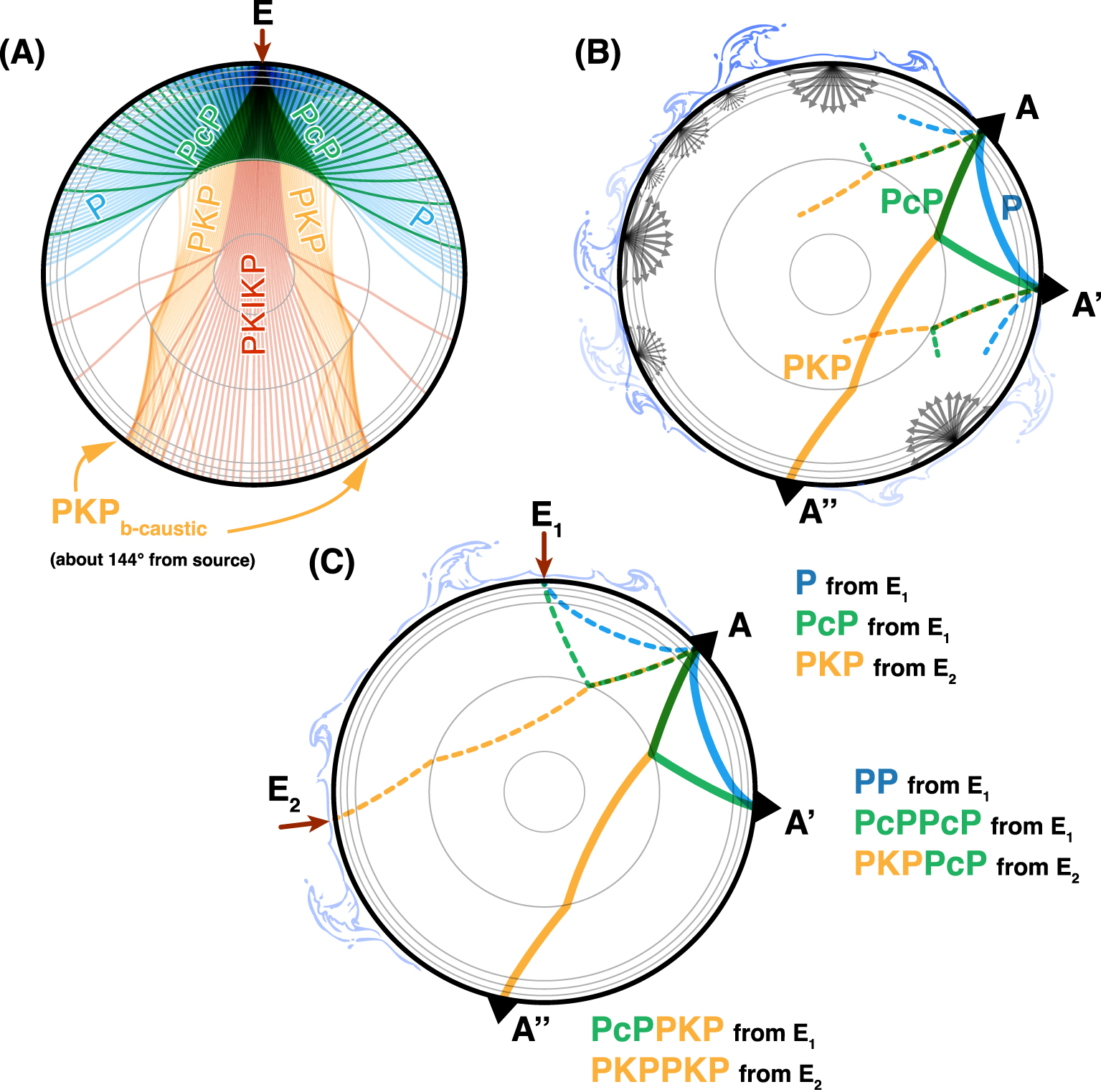
(A) Representation of ray paths for P, PcP, and PKP-type phases emanating from a source E located at the surface and computed within a radial Earth model for a regularly sampled take-off angle. (B) Schematic representation of the noise-based approach where multiple unknown sources are acting (also helped with a possible stacking procedure along continuous recordings). Under favorable conditions, the correlation between two stations could reveal GF-compatible phases like P, PcP between A and A′ or PKP between A and A′′. (C) Schematic representation of the proposed approach which relies on a careful data selection. Here, particular phases (like P, PcP, or PKP) are retrieved by specific interferences made from specific and known sources like E1 or E2 in this example. On all panels, the different types of seismic phases are organized by color. Dotted lines represent the incoming rays while solid lines correspond to the expected/targeted paths. Masquer
(A) Representation of ray paths for P, PcP, and PKP-type phases emanating from a source E located at the surface and computed within a radial Earth model for a regularly sampled take-off angle. (B) Schematic representation of the noise-based approach ... Lire la suite
For instance, Retailleau et al. [2020] reported clear observations of both P and PcP phases between seismic stations deployed in Europe and the USA after correlating one year of continuous data. These signals were interpreted as partial GF retrieval and used to produce a lower mantle image through migration techniques. Besides the obvious first-order time match with a 1D reference model, these two phases exhibited clear symmetry between the two propagation directions (respectively on both causal and acausal parts of the CCF). This symmetry of the correlation function was argued to be proof of CCF convergence toward the GF, thus justifying a direct application of migration technics. Such a noise correlation approach, illustrated in Figure 1B and initially developed for surface wave applications [Bensen et al. 2007], relies on the idea that for a given station pair (e.g., AA′), a sufficient stacking over continuous data will average the contributions from many sources. This idea is represented schematically in Figure 1B where many sources give rise to a (“noise”) field that contains P and PcP phases between A and A′, and PKP between A and A′′. The corresponding processing workflow is shown in Figure 2 (left panel). The resulting correlation wavefield will then contain GF-compatible ray paths, also producing symmetrical CCF. For instance, van Manen et al. [2006] showed and discussed at a smaller scale how the surrounding distribution of sources enables CCF convergence toward GF based on constructive stacking produced by the stationarity (over source integral) of travel-time difference (or phase) between two interfering seismic phases. At a large scale, this was further explored and discussed in the context of the so-called Earth’s correlation wavefield based on the coda of large earthquakes [Phạm et al. 2018]. In that study, the stationarity was explicitly associated with shared ray parameters for which Earth’s major discontinuities play the role of secondary (i.e., virtual) sources. This was also discussed in Li et al. [2020a] for microseism sources.
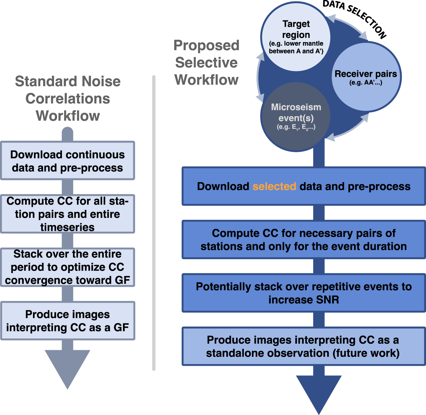
Schematic comparison between the standard noise correlation approach (left column) and the proposed selective workflow (right column). CC and GF stand for cross-correlation and Green’s function respectively, SNR for signal to noise ratio. The proposed approach relies on a data selection using the 3 main parameters: microseism events (date, location, strength), structural target and associated seismic phases (e.g., CMB/PcP), and corresponding receiver pairs that will support the necessary interference.
In the context of secondary microseisms, the distribution of sources located on the Earth’s surface is far from being even. Also, strong isolated sources, usually associated with significant cyclonic events [e.g., Farra et al. 2016, Retailleau and Gualtieri 2021] dominate continuous seismic recordings [e.g., Nishida and Takagi 2022]. Dominant sources are responsible for an unbalanced partition of energy between eigenrays reaching the two stations, which can lead to ambiguous phase measurements. As a result, final images are biased, if not erroneous. A non-symmetrical CCF will be the first obvious sign of such source effects, hence the argument of Retailleau et al. [2020] that symmetry is an indicator of CCF quality. But more subtle ambiguities also exist.
An example is shown in Figure 3 to illustrate the problem in a case that conforms to the observation of PcP phase, as in Retailleau et al. [2020]. We here use PcP as a target phase between station A and A′ (red path in Figure 3A). The reflection mid-point at the CMB between A and A′ is considered here as a target region. Following the idea and vocabulary introduced by Wang and Tkalčić [2020] in the context of long-lasting reverberations, a correlation “feature” (labeled PcP* in this case) is made from numerous constitutive interferences or “constituents”; each constituent being an interference between two coherent seismic phases, which can be reduced to a ray path difference under the ray approximation. Thus, constituents are named by simply associating the two interfering phases with a minus sign, the corresponding lag-time being the subtraction between the two initial phases. For example, PcPPcP-PcP (Figure 3A) refers to an interference matching a PcP phase between the two stations. Assuming that microseisms generate weak body waves which quickly drop below incoherent noise level, and contrary to the late coda of the large earthquakes [e.g., Tkalčić et al. 2020], only the direct wavefield and a limited number of reverberations (e.g., PP, PcPPcP, PKPPKP, PKPPcP, as illustrated in Figure 1C) are involved in the correlation wavefield. Note that no long-lasting reverberation is observed in the microseism frequency range due to both weak sources and rapid attenuation. It means that correlations are mostly sensitive to source dynamics (and primarily all their appearance and disappearance) and the same goes for ambiguities they contain as illustrated in Figure 3.
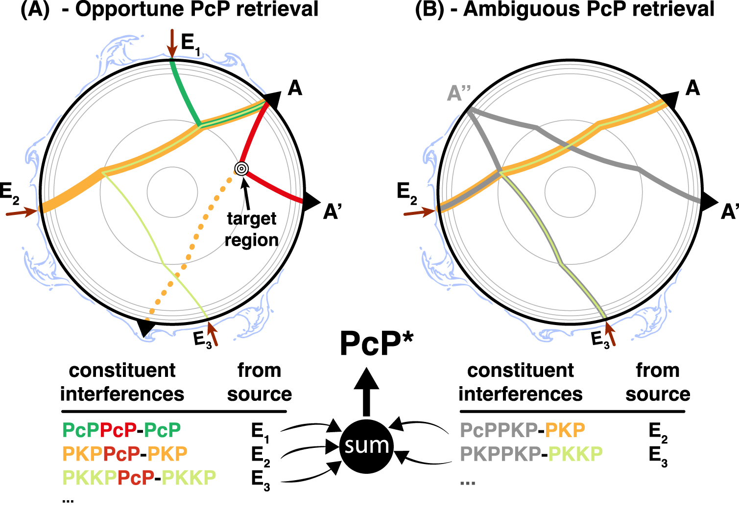
Illustration of possible ambiguities for a PcP* feature. Microseism sources are labeled from E1 to E3. A and A′ are the two considered stations. The targeted phase here corresponds to a PcP between A and A′. (A) Illustration of the main constituents of PcP* which indeed include the targeted PcP branch (in red). (B) Ambiguous constituents as they do not include the targeted PcP branch. Note that the same kind of ambiguities exists for any correlation features, such as PKP*, shown as a dotted yellow ray in (A). Masquer
Illustration of possible ambiguities for a PcP* feature. Microseism sources are labeled from E1 to E3. A and A′ are the two considered stations. The targeted phase here corresponds to a PcP between A and A′. (A) Illustration of the ... Lire la suite
The most intuitive constituents of a PcP* feature are PcPPcP-PcP and PKPPcP-PKP differential travel paths. These interferences are only possible in the case where sources are located at E1 and E2 respectively. If these two sources are contributing to the CCF, the resulting PcP* between A and A′ will be made from, at least, these two constituents. Because a reflection at the CMB is generally weak relative to the corresponding transmission into the core, we expect PKPPcP-PKP to be more effective to produce a PcP* feature. Several studies reported the major influence of PKP branches emanating from secondary microseism events [e.g., Li et al. 2020a]. For instance, PKKPPcP-PKKP can also contribute in the same way for a source located in E3. For these 3 constituents, the PcP* travel path is corresponding to the actual PcP between A and A′ (Figure 3A), meaning that these constituents are at least partly sensitive to the targeted path (discussion on spatial sensitivity in the last section).
As explained by Phạm et al. [2018] in a more generalized framework, a correlation feature is made from all possible constituents that are formed by seismic phases reaching A and A′ with the same ray parameter (condition of phases stationarity). Consequently, a constituent can be formed by two seismic phases that do not intrinsically contain a PcP between A and A′. This is for instance the case of PcPPKP-PKP from source point E2 or PKPPKP-PKKP from E3 (Figure 3B). Note that PKPPKP-PKKP does not include a PcP branch by itself, but rather a reflection of a “cP” branch on the surface, which by symmetry shares the same travel time as a PcP, thus contributing to the PcP* feature. This could of course be extended to any other correlation features such as P* and PKP*. It is important to note that this decomposition into constituent interferences underpins the classical GF retrieval from noise correlation for a closed system such as the Earth. Ruigrok et al. [2008] already proposed some pre-processing (multiple removals) to properly satisfy interferometric relations. Problems could be critical when CCF is blindly used from an initial source distribution that is dominated by some specific events. In that case, some constituents may become dominant and generate misinterpretation of the observed travel times and waveforms in terms of structural information: in other words, observations are not sensitive to the expected structure/location within the Earth.
To come back to the case of Retailleau et al. [2020], it is most likely that the observed PcP* between the US and Europe is dominated by a PKPPcP-PKP constituent that is formed by sources in the southern oceans. A single oceanic event following a prevailing Eastward trajectory south of Tasmania can indeed produce a PcP branch traveling in both directions below the North Atlantic. In other words, a source (E) transiting near E2 in Figure 3A could produce a PKPPcP-PKP constituent for the geometry E–A–A′ and then, depending on its trajectory and dynamic, for the reversed direction E–A′–A. This is by itself not a problem for imaging applications, the symmetry of the correlation is simply produced by a transit of the “same” source into the stationary zone (a.k.a. Fresnel zone, the area formed by the stationary condition of the phase difference for a given interference) of this constituent. Finally, the convergence of the PcP* observed by Retailleau et al. [2020] is probably not as complete as expected and very few oceanic events contribute to it over the entire year.
To avoid these complications, we here propose to restrict the number of constituents by only correlating localized events. Following the synthetic experiment proposed by Ruigrok et al. [2008] where they correlate wavefields produced by patches of sources, we show in the following sections that a single microseism event is sufficient to produce robust features in the correlation between distant stations.
3. Proposed workflow
Figures 1C and 2 illustrate the proposed workflow as a comparison with the classical noise-based approach, the latter being similar to surface wave applications. The main steps remain the same: downloading necessary data and correlating after some pre-processing. Differences are mostly in data selection. Where one could download continuous seismic data to facilitate, through stacking, the convergence of CCF to a more robust GF estimate, we here propose to only use a limited amount of data that we pre-select both in time and space according to three ingredients:
- a target structure (e.g., CMB in a given area) or a seismic phase (P, PcP, PKP …)
- the worldwide distribution of seismic stations
- our knowledge of the secondary microseisms (strength, date, location, spatial spread)
From here, it depends on the objective. Whereas a usual approach is to target a specific area, we here start from a particular microseism event to demonstrate the applicability of our workflow. One could easily adapt this workflow to other goals.
Knowledge of the source dynamics is critical to design an efficient strategy for data processing and avoiding ambiguous phase retrieval by adding unwanted constituents into the final correlograms, as discussed in the previous section. Numerous studies reported direct seismic observations of significant secondary microseism events, usually associated with major atmospheric depressions and oceanic storms. For instance, the seismic coupling of the super typhoon Ioke, which occurred in the late summer of 2006 in the western Pacific was detailed by several authors [e.g., Zhang et al. 2010, Retailleau and Gualtieri 2021, among others]. Such a significant event was proved to be very well predicted from sea state models. The source mechanism associated with secondary microseisms can be numerically computed from ocean sea state hindcast datasets when considering azimuthally dependent oceanic wave spectrum [Ardhuin et al. 2011, Ardhuin and Herbers 2013]. These numerical models usually show a good match with global seismic observations [e.g., Nishida and Takagi 2022]. Besides the state of the ocean swells, bathymetry plays an important role in the coupling between the ocean-generated pressure field and seismic waves [Longuet-Higgins 1950]. This amplification factor depends on several parameters other than the bathymetry itself: wave type and local velocity, considered frequency range and ray parameters (and thus local apparent wavelength). We follow derivations from Gualtieri et al. [2014] and use a P-wave amplification factor integrated over all possible ray parameters and computed at 6 s of period for this preliminary work. Finally, we focus on a single major event occurring in the North Atlantic on December 2014 that is already known to be seismically significant [Nishida and Takagi 2016]. In terms of secondary microseisms, the particularity of this northern Atlantic active area is linked to the combination of two factors: (1) an often adequate and very energetic sea state and (2) a good seismic coupling due to a complex bathymetry that produces a significant amplification factor over a large area overlapping storms’ trajectories.
Figure 4 shows the strategy to characterize source parameters from the ocean model. Figure 4A illustrates a portion of the sea state input model. Here, only the significant (ocean) wave height is shown at a given date (with a 3 h resolution). We can see the major impact of the storm between Iceland and Greenland where ocean swells reach values higher than 12 m on a very broad surface. The pressure field at the ocean surface is computed from the azimuthally dependent oceanic wave spectrum [Figure 4B, Ardhuin et al. 2011]. P-wave amplification coefficients are computed from local bathymetry (Figure 4C) and following Gualtieri et al. [2014]. Iso-values follow iso-bathymetry. Figure 4E shows modulation of the pressure field at the ocean surface by bathymetric amplification; this is interpreted as the actual pressure acting at the ocean bottom that applies to the crust and generates P-waves. On December 9, 2014, at 12:00 UTC, we can locate a very energetic source at about −33° E and 63° N (green star). We can also verify from our model that this location remains very active for the entire day. A better source characterization could be considered, but we rely on this first estimate to conduct our tests. Our modeling of this microseism event follows previous results from Nishida and Takagi [2016].
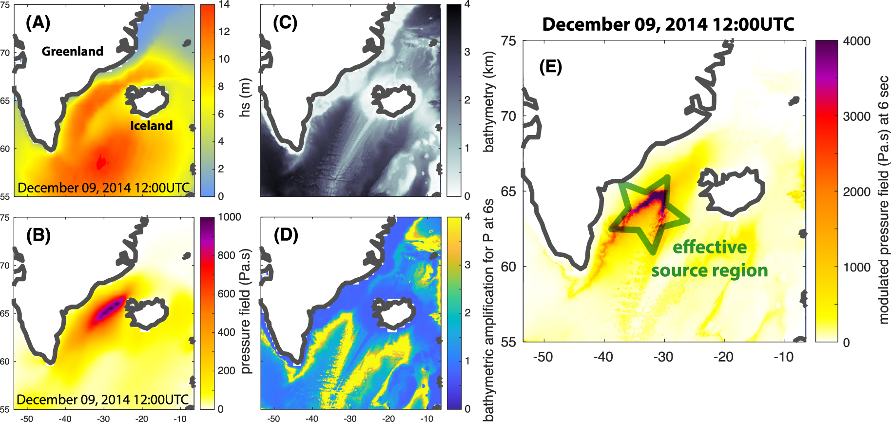
Illustration of the source characterization in the North Atlantic Ocean from the sea state model. (A) Significant wave height in the region on December 9, 2014 (12:00UTC). (B) Pre-computed pressure field from wave-wave interaction in open ocean derived from directional wave spectrum [Ardhuin et al. 2011]. (C) Local bathymetry (ETOPOv2). (D) The bathymetric amplification factor is computed for P waves at 6 s of period and intergrated over ray parameters following Gualtieri et al. [2014]. (E) Result of the effective source region from the modulation of panel (B) with (D). The green star corresponds to the most energetic area which we identify as the epicenter of this event at that date. Masquer
Illustration of the source characterization in the North Atlantic Ocean from the sea state model. (A) Significant wave height in the region on December 9, 2014 (12:00UTC). (B) Pre-computed pressure field from wave-wave interaction in open ocean derived from directional ... Lire la suite
Now that a source location and timing are known, we can select pairs of operational seismic stations worldwide depending on the targeted seismic phase (or constituent). For instance, let us again consider a pair of stations AA′ aligned on the great circle that includes source E and that would be spaced by the same distance that separates source E from the closest station A (e.g., the configuration of E1–A–A′ on Figure 1C). Such a combination would be perfectly suited for measuring constituents that are made by simple phase multiples reflecting at the Earth’s free surface such as PP-P, PcPPcP-PcP, or even PKPPKP-PKP when the inter-station distance gets long enough (Figure 1C). This geometry matches a stationary phase condition in the sense that the ray parameter of each phase reaching the sensors are similar. Since we work in a finite frequency range, the stationarity of the phase difference also allows the incorporation of some tolerance in the station selection: for a given source and a first station, a second station is searched in a small circle centered on the optimal point with a radius corresponding to 5% of the inter-station distance. This simple criterion accounts for the expected aperture of the stationary phase area on the source regions [see for instance Sager et al. 2022].
It is slightly more complicated for some other kinds of interferences. Let us consider a PKPPcP-PKP constituent (see E3–A–A′ configuration in Figure 1C). In that case, ray tracing is required. The ray parameter of PKP reaching the first station is used to compute the propagation distance of the PcP (with the same ray parameter) between the two stations. Using this distance, a forward geodetic arc is computed from the first station and following a great-circle direction to locate the optimal point to search a terminus station A′. As before, a tolerance area is kept when searching for a possible A′ station according to the expected stationary zone aperture. This ray-based data selection can be generalized to any others constituents. The sensitivity of final measurements to such a station pair selection according to the spatiotemporal properties of the source is outside of the scope of this study and will be further explored in future work.
Finally, seismic data are downloaded for the duration of a microseism event (typically from a few hours to a few days) and then correlated according to the previous selection. In the following section, all possible vertical components of high-sensitivity sensors (*HZ) are considered based on the International Federation of Digital Seismograph Networks (FDSN) archive. No particular processing is performed before correlation except for (1) an instrument response deconvolution and a resampling to 4 Hz after the application of an anti-aliasing pre-filter, to account for variability in instrument sensitivity; and (2) a spectral whitening in the period range of interest (from 3 to 12 s), to only measure the coherency of the phases and reduce the impact of relative amplitudes. Correlations are computed on an hourly time series and phase-weighted stacked [Schimmel and Paulssen 1997]. Since our selection of station pairs is oriented, only the causal part of the CCF is considered. Bathymetry plays an important role in the spatial distribution of sources. Some locations in the ocean with favorable bathymetry may produce redundant events over time even though the ocean sea state has a complex dynamic. In that case, a stacking procedure could be performed to enhance the signal-to-noise ratio (SNR). In the following, a single event is used as it is strong enough to show good SNR and validate the workflow. This workflow is summarized in the right panel of Figure 2.
4. Application and results
To illustrate the workflow, we choose a time window of 24 h starting on December 9, 2014, at 9:00 UTC, also knowing that such a significant ocean storm is seismically active for more than a day [Nishida and Takagi 2016]. Taking into account a longer time window could require re-evaluating the epicenter of the event, hence re-evaluating the optimal pairs of stations following the method described above.
Figure 5A illustrates our selection of station pairs considered to measure constituents involving a simple reflection at the Earth’s surface such as PP-P and PKPPKP-PKP (see Figure 1C). Because of this data selection, station pairs align naturally along great circle arcs including the source region (green star). Inter-station distances are color-coded from short, in black, to long, in light yellow. Red points are starting points (e.g., station A for event E1 in Figure 1C), and purple ones are terminus points (e.g., station A′ for event E1 in Figure 1C). At longer distances, for which we expect detection of PKPPKP-PKP (e.g., E2–A–A′′ in Figure 1C), terminus points can be close to the source region. Since surface waves are dominant close to the source, this geometry decreases our capability to detect weak body waves.
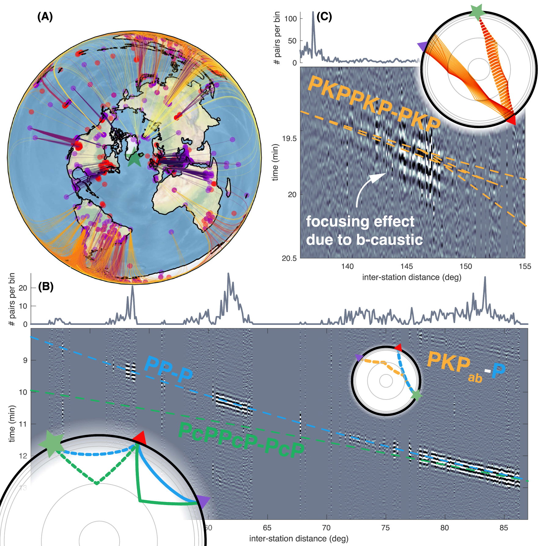
Results for station pairs selected based on their alignment with the source and an inter-station spacing matching single-phase multiples at the Earth’s surface. (A) Map of the effective station pairs selection centered on the source region (green star); inter-station distance is color-coded from black to light yellow. Red and purple dots are departure and terminus station locations respectively. (B, C) Seismic sections from cross-correlations stacked over a 0.1° distance bin. Ray tracing results matching each constituent are shown as dashed lines on both sections. Inserts showing slices of the Earth recall the ray path of each constituent as in Figure 1C. (B) Zoom on PP-P constituent. (C) Zoom on PKPPKP-PKP constituent. Masquer
Results for station pairs selected based on their alignment with the source and an inter-station spacing matching single-phase multiples at the Earth’s surface. (A) Map of the effective station pairs selection centered on the source region (green star); inter-station distance ... Lire la suite
Figure 5B shows a very coherent PP-P constituent that matches the prediction of a ballistic mantle P wave travel-time computed in a reference model [PREM, Dziewonski and Anderson 1981] using ray tracing from TauP toolkit for a corresponding inter-station distance [Crotwell et al. 1999]. Interestingly, no significant PcPPcP-PcP constituent is visible, despite the strength of this major source. As explained earlier in the context of the preliminary work of Retailleau et al. [2020], this is probably related to a relatively weak CMB reflectivity. In other words, observing both P and PcP in noise cross-correlation wavefield computed between two stations most probably corresponds to two different source regions. Some other coherent branches are visible. Before the PP-P branch, a significant arrival shows up (see at about 8.5 min, 80°). This matches a PKPab-P quasi-stationary constituent discussed by Li et al. [2020a]. A coherent signal at about 13 min, between 60° and 65° of distance may correspond to other constituents related to P-wave multiples. This composite seismic section shows a discontinuous coherency along the expected arrival times, which cannot be explained only by the stacking order within each bin. Complex local geology as well as other local sources in the vicinity of some stations, or simply non-isotropic source radiation in the far field may explain such differences in the coherency of the expected constituent for some pairs. This would require investigations and a quality check before any further exploitation of such signals for imaging applications. It is important to note that stacking pairs of stations according to inter-station distance is done for representation purposes, but a single pair of stations can show a very strong signal for a single ocean event already. Being able to detect a wavelet on a single station pair (or by using a local array) is critical for any 3D imaging application.
Figure 5C shows CCF for the same kind of station pair selection, but simply at larger distances where PKPPKP-PKP constituent is expected. Some significant coherency can be seen from 145° to 148°, which corresponds to the PKPb-caustic. At this frequency, it is difficult to decipher the different PKP branches’ contributions, but the caustic seems to play a significant role here as discussed by Snieder and Sens-Schönfelder [2015]. Some finite-frequency propagation modeling could help to see to what extent PKP-related constituents could constrain Earth’s structure. Again, it is worth reminding that only 24 h-long signals are used here, and stacking multiple events could help improve SNR.
Finally, we explore the feasibility of measuring PcP travel time based on a station selection that corresponds to a PKPPcP-PKP constituent (e.g., E2–A–A′ in Figures 1C and 3A). Figure 6A shows our data selection with a map projection that is centered at the sources’ antipode. A large number of temporary and permanent stations were initially present on a purely geometric selection, but a first-order quality check based on the SNR of the CCF left us with most station pairs between Australia and Antarctica. Local conditions of observations (southern oceans sea state), as well as the Antarctica ice cap, may explain the relatively low quality of observed signals. Figure 6B shows the PKPPcP-PKP constituent, zoomed over a portion of the available distant range. Our observation matches the expected PcP travel time, thus validating our station pairs selection. Again here, the quality of this composite seismic section does not seem to be correlated to the number of pairs stacked for building this section.
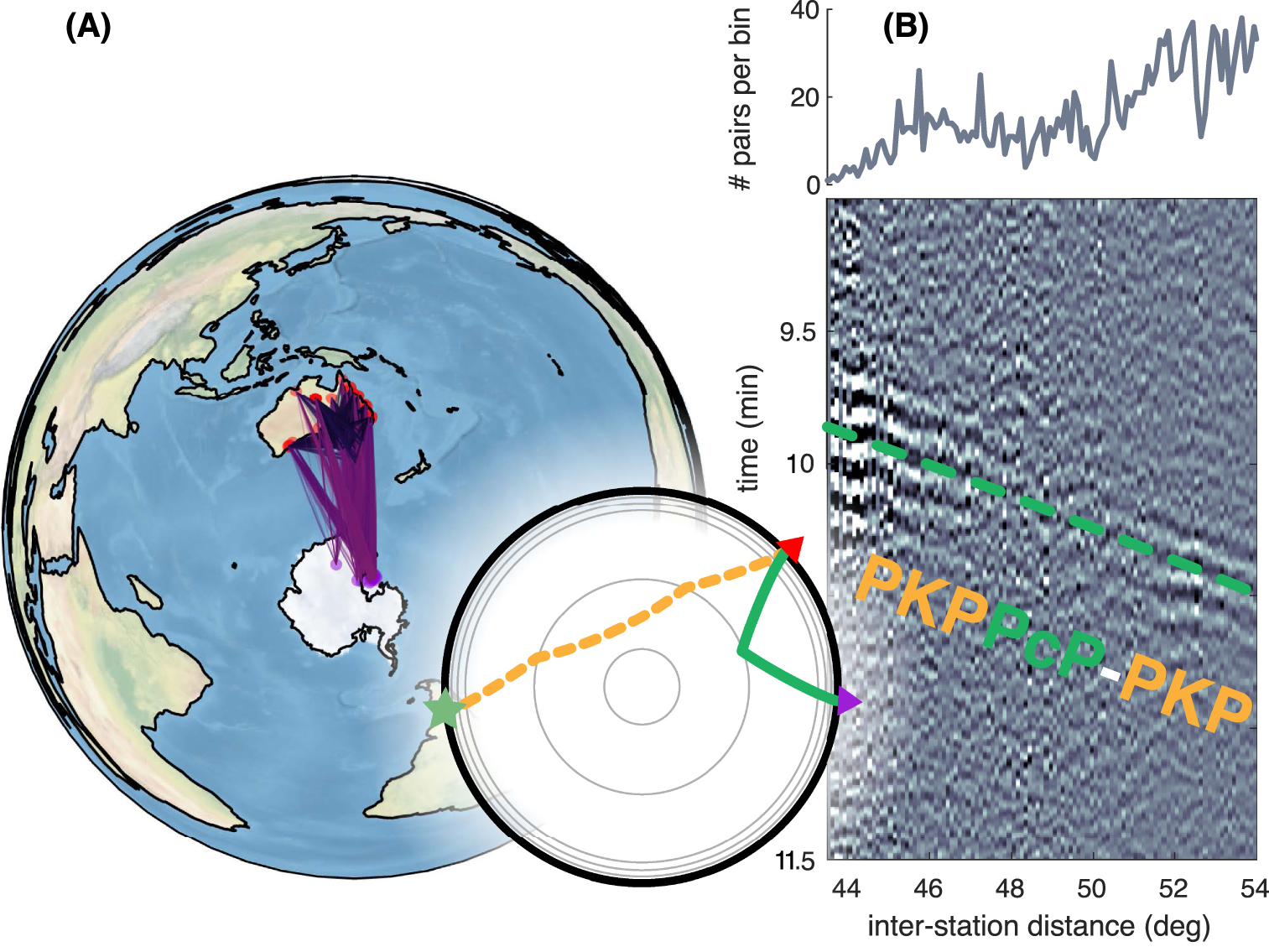
Same as Figure 5 but for a station pairs selection that corresponds to PKPPcP-PKP constituent which corresponds to PcP travel time. (A) Map of station pair selection centered on the antipode of the source location. (B) Seismic section from cross-correlations stacked over 0.1° distance bin zoomed on PKPPcP-PKP. Ray tracing results corresponding to a PcP arrival is shown as a green dashed line.
5. Discussions and conclusions
The proposed workflow revisits the idea of seismic daylight imaging [Rickett and Claerbout 1999, Schuster et al. 2004] and is also motivated by more recent successes of a noise-based correlation approach for the detection of teleseismic body waves in the secondary microseism frequency band. Here, cross-correlations are computed on carefully selected seismic station pairs for a given date and duration adapted to our knowledge of source patterns. Source parameters are derived from secondary microseisms computed from sea state models. The main goal of the proposed approach is to overcome some limitations of the noise-based correlation approach. Noise-based CCF can be biased and ambiguous because of the non-completeness of the necessary hypothesis of an isotropic incoming wavefield or source distribution. This is particularly important when teleseismic body waves are targeted. Misinterpretations emerge when a correlation feature with a travel time matching a known seismic phase (e.g., PcP) between the two stations is “blindly” interpreted as such. Following the decomposition of CCF features into constitutive interferences [Wang and Tkalčić 2020], we proposed an adaptative workflow to mitigate ambiguities for microseism event-based correlations.
A major microseism hitting North Atlantic Ocean on December 9, 2014, is used for illustrating the proposed approach. Pairs of stations are assembled according to various constituents: PP-P, PKPPKP-PKP, and PKPPcP-PKP. While such a large event is, by itself, sufficient to produce clear evidence of these constituents, multiple events could be stacked to improve SNR. Smaller events could then be used, helped by the fact that some areas are very prone to secondary microseisms over years, due to both storm periodicity and the dominant role of bathymetry for seismic coupling [e.g., Nishida and Takagi 2022].
Since different constituents can be measured independently, their interpretation is less ambiguous. The approximation of the GF between seismic stations is not an objective here, hence connecting measurements to the Earth’s structure is less straightforward. Since a single constituent is made from interference between two seismic phases, one needs to measure sensitivity to the structure of this differential path for imaging applications. Sager et al. [2022] estimated the sensitivity of such constituents in the context of fault monitoring, where crustal P-waves emanating from freight trains were correlated in California. Structural sensitivity of travel times measured from PP-P and P-P interferences were computed. This computationally intensive approach also enables a sensitivity evaluation of such measurements to source patterns. Similar evaluations should be performed at a global scale to make use of teleseismic constituents for imaging purposes. We can also emphasize the similarity of the microseism event-based SI approach discussed here with previous works on imaging and monitoring at smaller scales using timely passages of freight trains [Brenguier et al. 2019, Pinzon-Rincon et al. 2021].
It is important to note that even if an empirical evaluation of the GF between stations is not an objective, considering constituents based on a phase difference stationarity is critical because of the spatial extension of microseism sources. Again, stationarity appears when the constituent is made from seismic phases sharing the same ray parameters (e.g., P and PP when doubling the propagation distance), thus defining a possible finite frequency Fresnel zone. By definition, constructive interference happens for any source lying in (the main lobe of) this Fresnel zone. In a first approximation, the relatively large aperture of the stationary area in the secondary microseism frequency range (e.g., several hundreds of kilometers for PP-P at 50° inter-station distance and 6 s period) allows us to take advantage of each source spatial extent and time evolution. On the opposite, a spatially extended source outside the Fresnel zone would interfere destructively with itself due to the oscillatory nature of the interference for a finite frequency wavefield. Further work needs to be done to compare, for a given constituent, observed travel times with a prediction made from a combination of modeled sources and expected Fresnel zones. This is somehow related to the definition of microseism events themselves, which would also need some further investigations (time, space, strength, radiation …). We can also question the feasibility of inverting the interferometric scheme using its reciprocal form, following the idea introduced by Curtis et al. [2009]. The objective could then be to recover correlation features between two events by interfering them at a single seismic station aligned with these sources; but in this case, the (a priori) low correlation between the two source time functions of the two events will most likely be an obstacle for making significant detections.
Finally, this study shows that it is possible to observe teleseismic phases propagating from a single strong microseism source by correlating only a few hours of continuous recordings between station pairs selected for particular body-wave interferences (constituents). In other words, it is possible to turn a few hours of ocean-related non-impulsive tremors-like signals into a clear ballistic pulse in the far field. The limited frequency range of secondary microseisms as well as a dominant impact of some particular regions acting as significant microseism events (e.g., North Atlantic Ocean) are the main and foreseen limitations of this approach. Moreover, we noticed the lack of S-wave-related constituents in these preliminary results, despite the possibility to observe S waves in ballistic wavefields emanating from the same source [Nishida and Takagi 2016]. Horizontal components need to be explored to further conclude. Direct comparison with earthquake data is not straightforward because of the sensitivity of the constituents that are different from the GF between the two stations [Sager et al. 2022], but we expect these two datasets to be complementary. An opportune station pair selection could fill in some of the inherent lack of illumination produced by uneven source–receiver geometries when using earthquakes as sources for deep Earth imaging applications.
Conflicts of interest
Authors have no conflict of interest to declare.
Acknowledgments
We acknowledge the two anonymous reviewers and the editor Andrew Curtis for their thorough reading and useful comments. We also acknowledge the support from the French National Research Agency (ANR) under the project TERRACORR (ANR-20-CE49-0003). Maps are produced using the Cartopy package (doi:10.5281/zenodo.1182735). Bathymetry is taken from ETOPOv2c (doi:10.7289/V5J1012Q). Authors used subfunctions from Obspy within their processing workflow [Beyreuther et al. 2010]. The output of the ocean wave model can be found at http://ftp.ifremer.fr/ifremer/ww3/HINDCAST. We thank Fabrice Ardhuin and Mickaël Accensi for making this dataset available. We acknowledge all the people involved in seismic station deployment, maintenance, and data distribution worldwide. The list of all network codes used in the work is provided in supplementary material, as well as associated DOI.
Supplementary data
Supporting information for this article is available on the journal’s website under https://doi.org/10.5802/crgeos.222 or from the author.