

1 Introduction
There is a long history of studying noise within solid Earth seismology (Bonnefoy-Claudet et al., 2006). However, initially, the noise was not studied for its own merits. It was seen as a nuisance for studying the Earth through earthquake responses (Wilson et al., 2002) or for testing compliance with the comprehensive nuclear-test-ban treaty (Mykkeltveit et al., 1990). Hence, the noise studies were primarily concerned with understanding and suppressing the most disturbing type of noise, the microseisms. These microseims are ambient seismic vibrations related to swell waves in oceans.
Eventually, researchers realized that the noise itself can be used to study the Earth. In the second half of the last century, methods became popular to deduce Earth structure from noise, notably the spatial autocorrelation technique (Aki, 1965 ; Okada, 2003), the extraction of phase velocities from array measurements (Lacoss et al., 1969) and the horizontal-to-vertical spectral ratio technique (Nakamura, 2000). More recently, a technique was developed to turn noise from distant sources into a transient signal between two seismometers. This technique has been coined Green's function retrieval or seismic interferometry (SI) (Larose et al., 2006; Schuster, 2009; Snieder et al., 2009; Wapenaar et al., 2010). For example, Shapiro et al., 2005 used surface-wave microseismic noise from the Pacific to create a transient surface-wave record between stations in the Western USA. Subsequently, using surface-wave inversion, they obtained a velocity model of the crust.
Because of the developments of the above methods, noise is more and more considered a merit rather than a nuisance. Consequently, the recent noise studies focus on a wider frequency range than just that of the microseisms. Moreover, the body-wave portion within the noise is gaining more attention.
Already in the 1960s, Toksöz and Lacoss (1968) found that body waves dominated the noise between 0.4 and 0.8 Hz, for an array measurement in Montana, USA. Soon after, Vinnik (1973) studied microseisms recorded in Kazakhstan. For this array, in the middle of the continent, he found that, from distant oceanic sources, no Rayleigh waves were recorded, but just P-phases. Recent studies have shown that body waves are in fact omnipresent in ocean-generated noise. Roux et al. (2005) identified direct P-waves after crosscorrelating low-frequency noise. Gerstoft et al. (2006) found body waves in the double-frequency microseism band and could attribute these to P-phases induced by hurricane Katrina. They made these noise recordings with an array in southern California. In a later study, using the same array, they also found PP− and PKP phases in noise recordings (Gerstoft et al., 2008). They concluded that the body waves are induced year round and at many locations in the oceans. Landes et al. (2010) reached the same conclusions, using arrays in Turkey, Yellowstone and Kyrgyzstan. Zhang et al. (2009) found also a large proportion of body waves in noise between 0.6 and 2.0 Hz. Koper et al. (2010) used a worldwide distribution of arrays to study one year of noise. Per array, a small frequency band was chosen to beamform (Rost and Thomas, 2002) noise records. The frequency band depended on the spatial sampling of the arrays and varied within 0.5 and 4.0 Hz. For many of the arrays, besides the usual surface waves, a small portion of body waves was found. For some arrays, e.g. the ILAR array in Alaska, body-waves prevailed throughout the year.
The confirmation of the presence of body waves in low-frequency noise has made the noise more attractive for lithospheric imaging and even for exploration. Roux et al. (2005) considered the use of regional P-wave noise for tomography, after the application of SI. Zhang et al. (2010) demonstrated the use of teleseismic P-wave noise for obtaining a lithospheric velocity model through tomography. Zhan et al. (2010) obtained S-wave Moho reflections through interferometrically processing noise records. Draganov et al. (2007, 2009) used higher-frequency (>1 Hz) noise to compose an exploration-scale reflection response. The retrieved responses were subsequently migrated to obtain a reflectivity image of the subsurface. If non-volcanic tremor may be counted as noise, then Chaput and Bostock (2007) also used noise to retrieve scattered body waves between stations. With the retrieved responses they could confirm structure at about 10 km depth.
From the point of view of hydrocarbon exploration, high-resolution seismic reflection data is the most important exploration tool. However, increasingly, companies integrate various types of data to paint a more complete picture of the potential reservoir. In most cases, regional geological information also plays a role in the evaluation of the hydrocarbon potential of a basin.
It is with these observations in mind that we study noise in the frequency range [0.03–1.0] Hz, recorded with an array in Egypt. We split up the noise in different frequency bands, encompassing the primary and secondary microseism and higher-frequency natural noise. This division is based on the potentially different origins of the noise for different frequencies. Our aim is to determine whether we can use the noise recorded in one or more of these frequency bands for SI.
From the theory behind SI we know that a favorable source distribution is required to extract meaningful responses from the noise (Wapenaar and Fokkema, 2006). Our primary goal is therefore to characterize the noise and identify–where possible–its source areas, so as to evaluate the illumination of the array. To this end, we split up the noise records in small time windows and apply beamforming to determine the slowness and azimuthal distribution of the noise. A rough estimate suffices, since the exact source locations are not relevant for SI (Wapenaar and Snieder, 2007). To further distinguish between surface-waves and body-waves, we perform the beamforming for all three components and additionally compute the power-spectrum density variations for all three components. The noise records with a favorable body-wave content are processed into reflection responses.
2 Survey area and data inspection
An array of three-component stations was installed in an area over the Northeast Abu Gharadig Basin in the Western Desert in Egypt. This location is about 230 km west of Cairo. While the area is unpopulated, there is some activity related to oil-and-gas production. Although several tracks in the area were being used by traffic from local producers, the nighttime was very quiet.
Fig. 1 depicts the receiver layout. One hundred and ten broadband seismometers (Trillium T40) were placed in five parallel lines and three cross lines at varying angles. Inline interstation spacing was 500 m, with a more densely sampled (350 m) area in the middle of the array. In total, more than 40 hours of noise were simultaneously recorded on all 110 stations. The total survey area was about 60 km2.
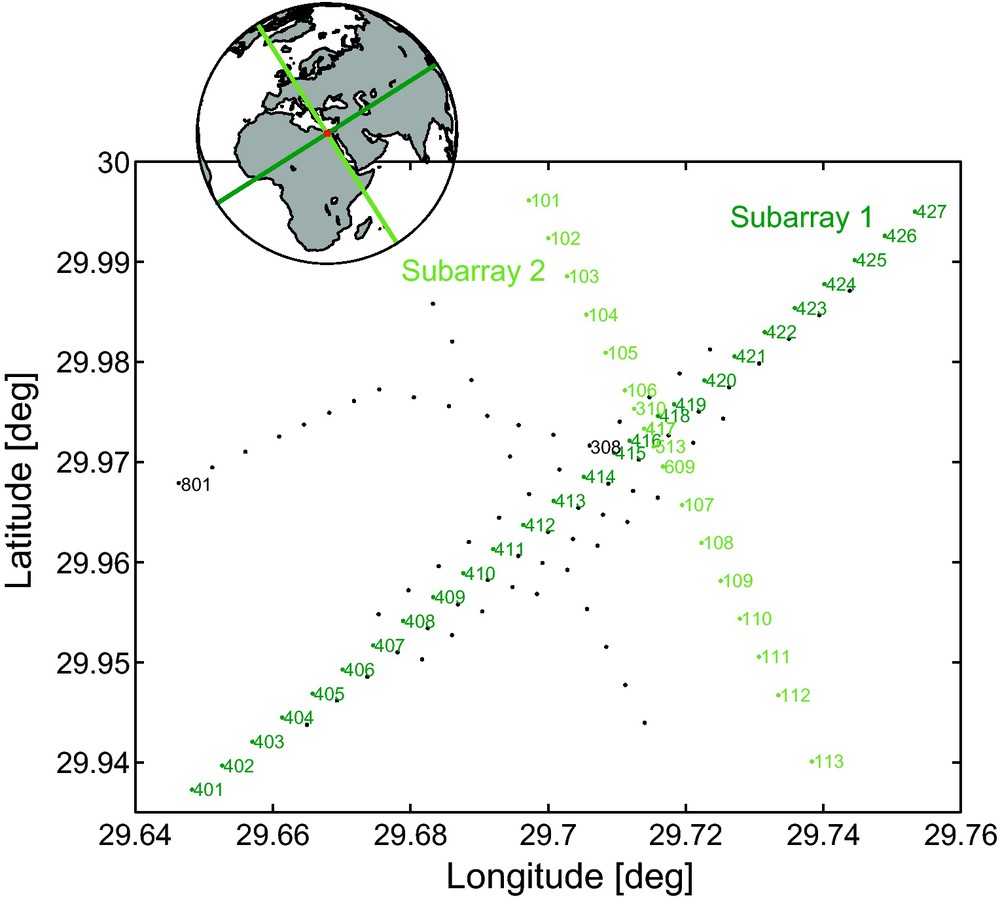
The Egypt-array configuration. The 110 three-component stations are denoted with black dots. The stations for various subarrays are coloured and numbered. In the inset, the bearings of the different subarrays are shown as rhumb lines on a worldmap.
Configuration du réseau égyptien. Les 110 stations à trois composantes sont matérialisées par des points noirs. Les stations des différents sous-réseaux sont colorées et numérotées. Dans l’encart, les directions de visée des différents sous-réseaux sont figurées par des loxodromies sur un planisphère.
Most of the stations are installed on a gravel plane. However, between stations 420 and 423 there is one significant sand dune crossing subarray 1. In general, the topography is slightly undulating, but not to the extent that station corrections are required to account for it.
We start our data analysis by comparing our array measurements with worldwide measurements of ambient noise (Peterson, 1993). We compute power spectral densities (PSDs) with the recipe given in the above reference. A selected spatial distribution of the resulting PSDs is shown in Fig. 2. The PSDs are compared with the New Low Noise Model (NLNM) and the New High Noise Model (NHNM) from Peterson (1993), whose values are obtained from Bormann (1998).
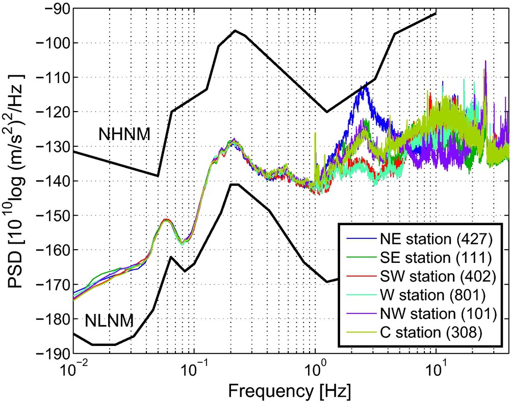
Spatial variation of the power spectral density (PSD) for the Egypt array. The PSDs are compared with the new low noise model (NLNM) and new high noise model (NHNM) from Peterson (1993) (solid black lines). The PSDs are expressed in ground acceleration, which was computed from velocity recordings.
Variations spatiales de la densité spectrale de puissance (PSD) pour le réseau égyptien. Les PSDs sont comparées avec les nouveaux modèles de bruit à basse niveau (NLNM) et à haute niveau (NHNM) selon Peterson (1993) (lignes noires continues). Les PSDs sont exprimées en accélération terrestre, calculée à partir des enregistrements de vitesse.
We observe a large similarity of the PSDs for the different stations between 0.01 and 1 Hz as opposed to large differences above 1 Hz. For many parts of the world 1 Hz separates the domain of domination by natural sources from a domain of domination by anthropogenic or cultural sources (Asten and Henstridge, 1984; Gutenberg, 1958). The distant natural noise sources (f < 1 Hz) are recorded similarly by all the stations, whereas the more nearby cultural noise sources (f > 1 Hz) are recorded with strongly varying amplitudes, e.g., the noise at around 2.5 Hz is stronger in the northeastern than on the southwestern side of the array, pointing to relatively nearby sources at the northeastern side. Most likely, it concerns car traffic.
For a further analysis, we will leave out the frequency band [1.0–40.0] Hz, due to its complicated nature and an interstation separation that is not particularly suited for further multichannel processing at these higher frequencies.
The noise records below 1 Hz follow the global trend, indicated by the NLNM and NHNM. The single-frequency (SF) and double-frequency (DF) microseismic peaks can well be distinguished, at 0.058 and 0.21 Hz, respectively. Both peaks are related to storms crossing the oceans (Tanimoto and Atru-Lambin, 2007). The SF peak is thought to be induced primarily when a storm traverses continental margins (Cessaro, 1994). Due to the relatively small water column, storm-induced ocean waves (swell) can couple directly with the ocean floor and hence induce seismic waves, which can be recorded thousands of kilometers away from the source. The DF microseism is thought to be induced at many places in the oceans, also at locations with large water columns (Vinnik, 1973). Single storm-induced ocean waves do not lead to pressure variations at large depths. However, when ocean waves collide, a pressure variation does build up at the ocean floor, with double or triple the frequency of the individual waves (Longuet-Higgins, 1950). This pressure variation couples to the solid Earth with seismic waves that are significantly stronger than the waves induced at SF (Fig. 2). Despite the fact that the DF-microseism noise could be induced anywhere in the ocean, it tends to be stronger near coasts. Specific coasts are good reflectors for ocean waves and hence provide the necessary opposing waves (Bromirski, 2001).
For the Egypt array, the SF and DF observation are closer to the NLNM than to the NHNM. This is not surprising, considering the distance to oceans with large storms. The nearby Mediterranean and Red Sea are relatively quiet, even in October.
For our analysis, we only use the times for which all the stations were active and good quality data were recorded. The starting time of this period is 12 October 2009 14:00, which we set as time zero.
For obtaining a helicopter view of the noise record, we compute the PSD for one station (no. 402) as function of time. The 40 h of continuous data are split up in windows of 10 min. For each of these windows the PSD is computed, using eight 75% overlying segments of 214 samples. The resulting functions are plotted as function of time, yielding the noise spectrogram as displayed in Fig. 3.
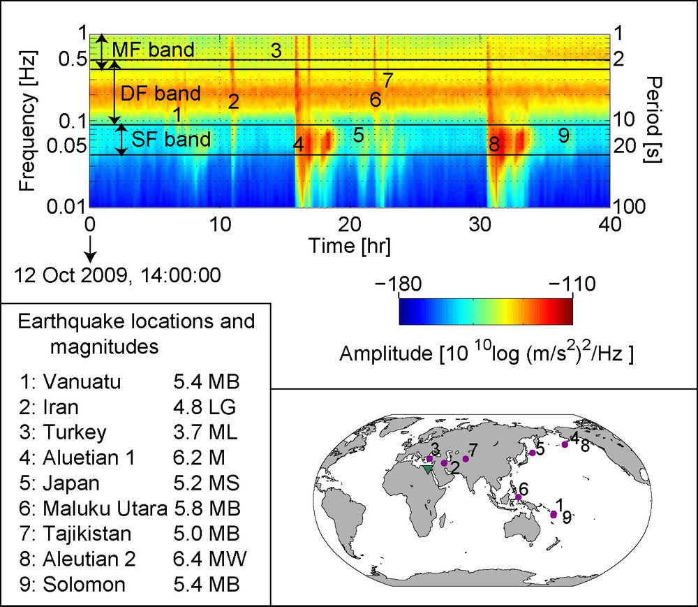
The noise spectrogram (upper figure box), made up by a concatenation of power-spectrum densities (Fig. 2) based on 10-minute Z-component records detected at station 402. The transient events are caused by earthquakes. The identified earthquakes and their magnitudes (given in various scales) are listed in the lower-left box and are indicated on the spectrogram. Their locations are plotted on a world map (lower-right box). The data between 0.03 and 1.0 Hz are divided into three frequency bands (MF, DF and SF) marking different characteristics of the noise in the various bands.
Spectrogramme de bruit (panneau en haut de la figure) bâti à partir des densités de spectre de puissance (Fig. 2), basées sur les enregistrements à composante Z sur 10 minutes, détectés à la station 402. Les évènements transitoires sont causés par des tremblements de terre. Les tremblements de terre identifiés et leurs magnitudes sont listés dans le panneau en bas et à gauche et sont indiqués sur le spectrogramme. Leur localisation est reportée sur un planisphère (panneau en bas et à droite). Les données entre 0,03 et 1,0 Hz sont divisées en trois bandes de fréquence (MF, DF et SF) marquant différentes caractéristiques du bruit dans ces bandes.
Within the 40 hours window, we identify all the large earthquake responses. The origin of all peaks below 1 Hz could be found by raytracing arrival times from earthquakes in a global catalogue (IRIS earthquake browser). All the identified source locations are plotted in the lower-right map in Fig. 3.
As in Fig. 2, we can easily identify the SF and DF microseism in Fig. 3. The DF microseism pops out as a stable ridge, marking its stability over time. The SF is significantly smaller and more hilly, marking a larger time variation.
The different types of noise are restricted to limited frequency bands. Hence, for the further analysis and processing, we split up the data in a few distinct frequency bands, as depicted in Fig. 3. The first band is chosen around and named after the SF microseismic peak (SF band, [0.03–0.09] Hz). The second band encompasses the DF microseismic peak (DF band, [0.09–0.5] Hz). In Fig. 2, it can be seen that, below 1 Hz, there is a small third hill, peaking at 0.55 Hz. We choose the third band (MF band, [0.4–1.0] Hz) such that it encompasses this hill. This MF noise gains in strength from about 30 h onwards (Fig. 3).
3 Origin of noise
Within the 40-h window (Fig. 3) we now identify the origins of the noise. We do this by splitting up the 40 h in non-overlapping time windows. We choose 10-min windows for the SF and DF band and 5-min windows for the higher-frequency MF band. Subsequently, each time window is beamformed.
The beamforming is derived and explained in a large number of references, e.g., Lacoss et al. (1969); Rost and Thomas (2002). Here, we only state the two basic steps. As a preprocessing step, a time window and frequency band is selected from an array measurement. As a first step, all traces for this selection are mutually crosscorrelated. Hence, a crosscorrelation matrix is obtained which contains all the time differences between different waves arriving at the different stations. As a second step, these time differences are fit with a forward model. As a forward model, bandlimited plane waves with varying backazimuth θ and rayparameter p are considered. The degree to which the model fits the data is expressed in beam power. Thus, after beamforming, the beampower is obtained as a function of backazimuth and rayparameter. The p and θ with the maximum beampower is chosen as the dominant rayparameter pdom and the dominant backazimuth θdom, respectively.
The beamforming is implemented in the frequency domain (Lacoss et al., 1969). Instead of computing the beampower for each frequency sample individually, the frequency band is split up in bins and the beampower is only computed for a stack of the frequency samples within each bin. This procedure stabilizes the estimate. We choose five frequency bins per frequency band. For obtaining the final beampower, the beampowers for the different bins are stacked.
Fig. 4 shows an example of beampowers for the three different frequency bands we consider. The beampowers were computed using the first time window of hour 26 (Fig. 3). In Fig. 4a–c, the array signature can well be noted. The beampower has a higher resolution on the SW-NE than on the NW-SE transect due to a better coverage of stations on the former transect. Also, the difference in resolution is obvious for the different frequency bands. Nevertheless, a clear pdom and θdom can be picked for each frequency band.
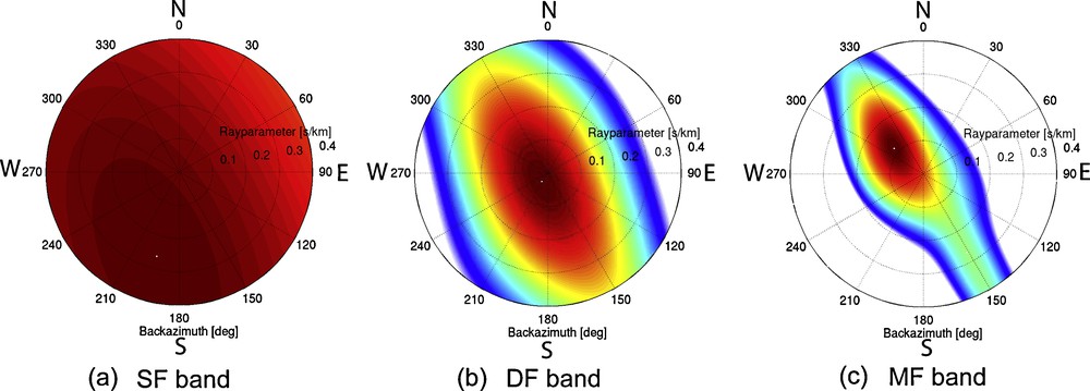
A beampower output for (a) the SF band (using the first 600 s in hour 26), (b) the DF band (using the same time window) and (c) the MF band (using the first 300 s in hour 26). Taking the maximum beampower value, for the SF band, we find: θdom = 185°, pdom = 0.251 s/km, for the DF band: θdom = 216°, pdom = 0.031 s/km and for the MF band: θdom = 311°, pdom = 0.117 s/km.
Puissance obtenue par formation de voies pour (a) la bande SF (utilisant la première fenêtre de temps de 600 secondes dans l’heure 26), (b) la bande DF (utilisant la même fenêtre de temps) et (c) la bande MF (utilisant les premières 300 secondes dans l’heure 26). En prenant la valeur maximum de la puissance de faisceau, on trouve: θdom = 185°, pdom = 0,251 s/km, for the DF band : θdom = 216°, pdom = 0,031 s/km and for the MF band : θdom = 311°, pdom = 0,117 s/km.
Note that, within the chosen time window, waves of similar strength, but from different sources or with different raypaths, might arrive. If this is the case in the SF band, beampowers from the different waves will inevitably interfere, due to the low resolution (Fig. 4a). For smaller distances in the p–θ plane, beampower interference will also occur in the DF- and MF-band (Fig. 4b,c). The longer time-records are included in the beamforming, the more different waves will arrive and the more severe the interference will be. Hence, we choose relatively small time windows to increase the chance to yield parameters of individual noise sources rather than averages over multiple sources.
After beamforming and automatic picking we obtain pdom and θdom for all time windows and frequency bands. Fig. 5a and b show the resulting backazimuth and rayparameter distributions, respectively. We interpolated the distributions for the SF- and DF- to achieve the same number of total counts as in the MF band.
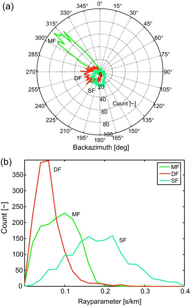
(a) A rose diagram of the dominant noise directions and (b) a distribution plot of the dominant rayparameters, for the three different frequency bands of interest (Fig. 3). The directions and rayparameters were estimated by beamforming 40 h of data.
(a) Diagramme polaire des directions de bruit dominant et (b) schéma de répartition des paramètres de rais dominants, pour les trois différentes bandes de fréquence prises en considération (Fig. 3). Les directions et les paramètres de rai sont estimés en considérant 40 heures de données pour la formation de voie.
In all frequency bands prevailing noise directions exist. Noise from the direction of the Mediterranean dominates the MF band (and hence its name, Mediterranean Frequencies), whereas the SF- and DF-band seem to be susceptible to noise from especially the southern Atlantic.
The rayparameter distribution (Fig. 5b) is rather broad for all bands considered. For body-wave seismic interferometry, the DF- and MF-band show the most favorable distribution, as we will see in the next section. The SF band contains primarily surface waves and is therefore considered to be unsuitable for body-wave SI.
In the following, we will first introduce noise SI and better analyze the wavemode content in the noise, before moving onwards to the actual SI processing. The analysis of the DF band (Section 5) is used to introduce our noise-analysis method.
4 Noise SI
In our configuration we have receivers on the free surface, above the medium of interest (Fig. 1). Also the noise sources are at or near the free surface. However, because of the distance of the sources and the velocity gradient in the crust and mantle, effectively the medium of interest is illuminated from below. For this configuration, Wapenaar and Fokkema (2006) derived interferometric relations. They found that the noise can be used to retrieve the Green's function between two receivers when the noise sources are mutually uncorrelated and a long time window of noise contains a good spatial distribution of noise sources. For details about the required distribution of sources, we refer to Ruigrok et al. (2010). In practice, the second condition is unlikely to be fulfilled. Even if there were a perfect source distribution then the estimated Green's function would still be biased by differences in strength of the sources. To compensate for this, we split up the noise record in small time windows (panels) and root-mean-square normalize each panel. We make the assumption that each such panel is dominated only by a single noise source. This assumption is checked with beamforming (Section 3).
For SI, we threat different phases from the same source as different effective sources illuminating the medium of interest with different angles of incidence. The wavefields due to the noise sources are assumed to be planar near the array. Hence, an effective source is parameterized with the beamforming output p = (pdom,θdom), where pdom and θdom are the dominant rayparameter and backazimuth of the noise. If a certain panel contains multiple strong beams of similar energy, this panel is rejected. For the accepted panels we can write the noise registration at stations xA and xB as:
| (1) |
| (2) |
| (3) |
In the following, we will binarize the azimuthal dependence in relation (3). At the positions halfway between xA and xB, the globe is divided into two hemispheres. For illumination from the hemisphere on which xA is situated, the rayparameter gets the addition of a superscript +, whereas for illumination from the other hemisphere the rayparameter get the addition of a superscript −. In the following, the subscript dom is left out to simplify the notation. When we assume that the medium is approximately layered, Eq. (3) can now be split up into two equations:
| (4) |
| (5) |
Our goal is to retrieve reflections from a wide source-receiver offset range. Most of the lithosphere is approximately horizontally layered. In this case, a zero-offset reflection response corresponds to p ≈ 0. Consequently, to obtain this response, we also need illumination with pmin ≈ 0. The required Pmax is dictated by the largest source-receiver offset 2 h and the shallowest interface d of interest (Fig. 6).
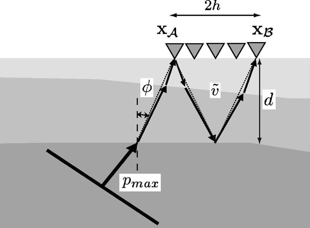
Configuration for the computation of the required rayparameter (Eq. (6)). The tilted line in the lower left denotes a plane-wave, illumination a two-layers-over-a-half-space model. Only the rays (denoted with arrows) are drawn that connect the outer two receivers of the array via a bounce from the second interface. The rays are the actual raypaths while the dotted lines would be the raypaths if the upper two layers were replaced by a layer with their average properties.
Configuration pour le calcul du paramètre de rai (Éq. (6)). La ligne en arête de toit en bas et à gauche indique une onde plane, modèle d’illumination de deux couches sur un demi-espace. Seuls sont dessinés les rais qui relient les deux capteurs externes du réseau via un rebond sur de la seconde interface. Les lignes en couleur sont les trajets des rais, tandis que les lignes en pointillés seraient les trajets si les deux couches supérieures étaient remplacées par une couche avec leurs propriétés moyennes.
The largest offset would ideally be the offset between the two outer receivers in the array. The shallowest interface that could be observed is restricted by the band limitation of the noise and interfering effects from correlations of direct waves. Consequently, reflections from the shallowest interfaces can normally not be retrieved. Fig. 6 shows the stationary illumination (Snieder, 2004) with a plane-wave source for the retrieval of a primary reflection from the second interface. We can express the rayparameter of this reflection as , where is an average velocity of the first two layers. Combining this last expression with yields
| (6) |
As long as the illumination range [pmin, pmax] is well sampled pmax may be much larger than dictated by expression (Eq. (6)). However, since we are interested in reflections only, we always choose pmax < 0.20 s/km, which would be the rayparameter for a direct P-wave with a velocity of 5 km/s. Hence, we do not retrieve surface waves, which we otherwise would need to filter out again before migrating the retrieved responses.
5 DF band
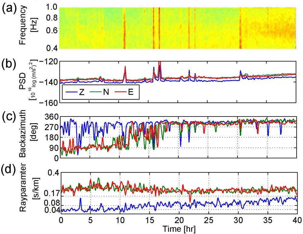
We start the analysis of the data in the DF band ([0.09–0.5] Hz) by computing the PSD time-variation function, as in Fig. 3, but now only for the DF band and for all three components. The PSD time-variation function for the Z-component at station 402 is plotted in Fig. 7a. With this plot we can study the amount of energy that is recorded for certain time intervals. Especially, we can study to what extent this energy is distributed over the entire frequency band.
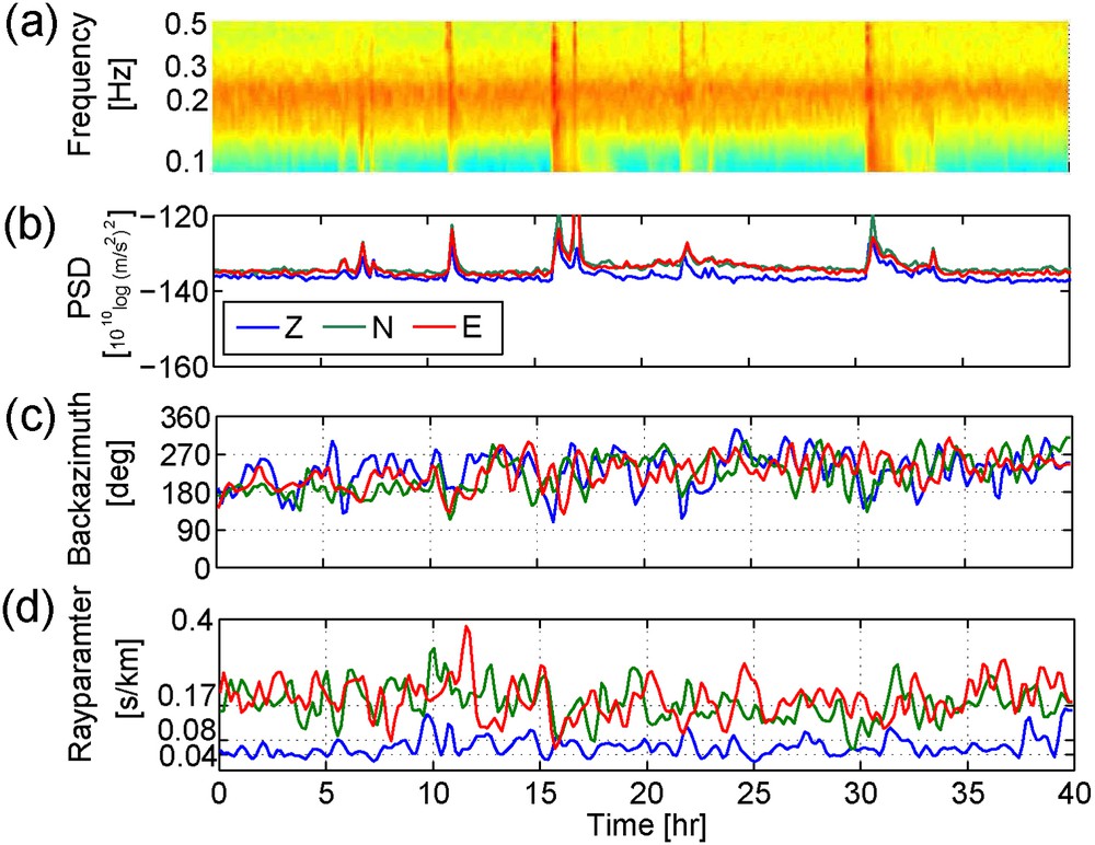
DF-band noise-variation plots for 40 h of data, starting 12 October 2009 at 14:00. (a) Power spectrum density (PSD) variation on the Z-component and, for all components, (b) the averaged (over frequency) PSD variation, (c) the backazimuth and (d) the rayparameter variation.
Représentation de la variation de bruit dans la bande DF pour 40 heures d’enregistrement, débutant le 12 octobre 2009 à 14 heures : (a) variation de la densité spectrale de puissance (PSD) sur la composante Z et, pour toutes les composantes, (b) variation de PSD moyennée sur le bande de fréquence, (c) l’azimuth en retour et (d) la variation du paramètre de rai.
Fig. 7b shows averages over frequency of the PSD time-variation functions. For each time interval, the average of the PSD within the DF band is shown for the Z-component (blue line), the N-component (green line) and the E-component (red line). Hence, on this plot we can study the differences in recorded energy for the different components.
Fig. 7(c) and (d) shows the time-variation graphs for the estimated θdom and pdom, respectively. To make these graphs, the beamforming on the Z-component (as introduced in Section 3) has been repeated for the N- and E-components. The graphs have been smoothed using sliding average of three-sample windows. Similar pdom for the different components would indicate the measurement of the same (mix of) wavemodes on all components. A similar θdom for the different components would hint at a susceptibility to a similar source (or mix of sources).
One important element for noise characterization in general is estimating the contribution of surface and body waves (Bonnefoy-Claudet et al., 2006). Using the four plots of Fig. 7 together, we can untangle the noise for a large part. Making the assumption that the noise sources are near the Earth's surface and far away we can already largely classify the arrivals based on their rayparameter (Fig. 8). Rayparameters below 0.173 s/km can only be explained with body waves, whereas rayparameters above 0.312 s/km can only be explained with surface waves. Rayparameters between 0.224 and 0.312 s/km are harder to classify, since they could be explained by both surface waves and local S-phases. For this p-band, Fig. 7b helps out.
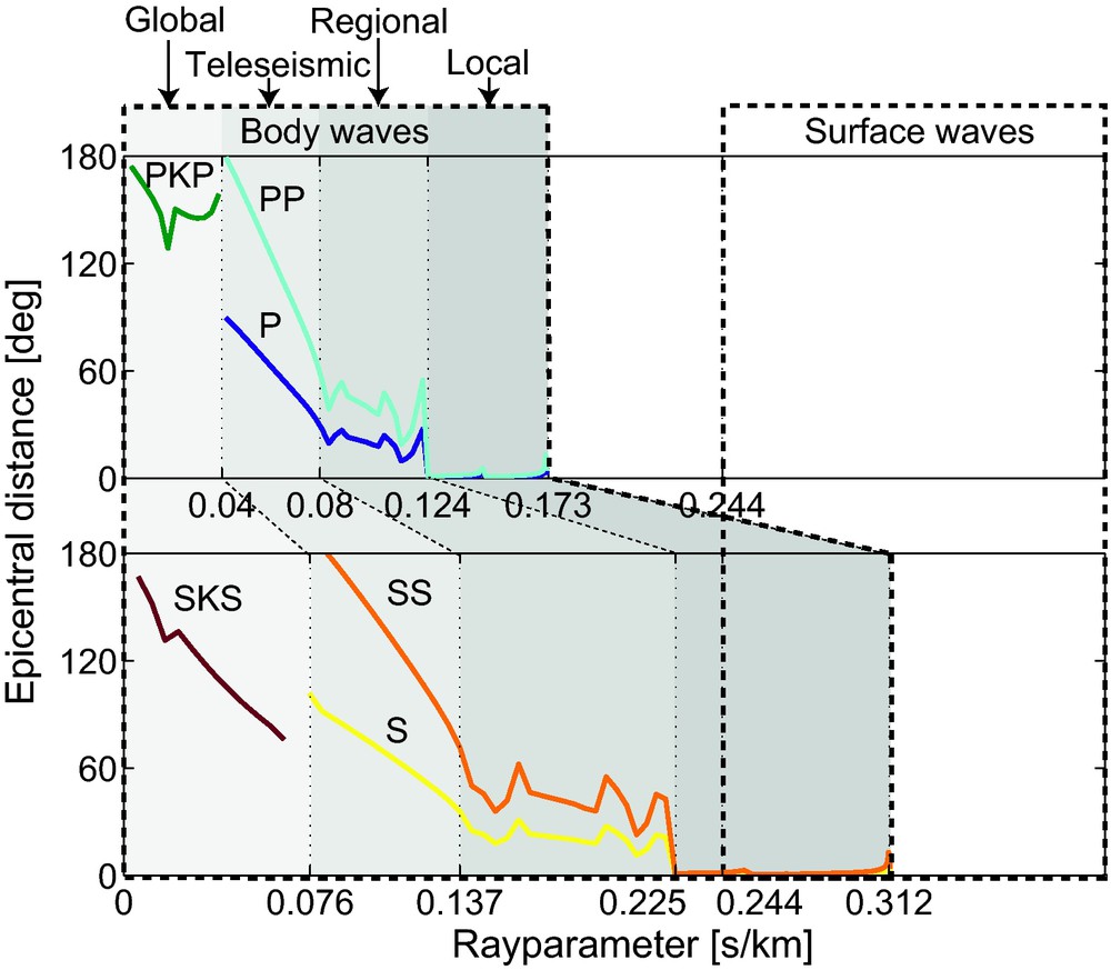
Classification of phases based on rayparameter. For body waves, the four considered classes (indicated with grey shading) are based on the depth penetration of the waves. The four classes are global, teleseismic, regional and local, for waves reaching until within the core, the mantle, the lower crust and the upper crust, respectively. In the upper figure, the rayparameter versus distance graphs are shown for the most energetic P-phases, whereas in the lower figure the same functions for the most energetic S-phases are shown. The functions were computed with TTBox (Knapmeyer, 2004) using a 1D Earth model (PREM, Dziewonski and Anderson, 1981). Using the same model, the lower rayparameter bound for surface waves (0.244 s/km or 4.10 km/s) was computed for a fundamental-mode Rayleigh wave with a peak frequency of 0.01 Hz.
Classification de phases basée sur le paramètre du rai. Pour les ondes de volume, les quatre classes considérées (indiquées par des zones ombrées) sont basées sur la profondeur de pénétration des ondes. Les quatre classes sont globale, télésismique, régionale et locale, pour les ondes atteignant le noyau, le manteau, la croûte inférieure et la croûte supérieure, respectivement. Dans la partie supérieure de la figure, les diagrammes du paramètre de rai en fonction de la distance concernent les phases P les plus énergétiques, tandis que dans le bas de la figure, ce sont les mêmes fonctions pour les phases S les plus énergétiques qui sont présentées. Les fonctions ont été calculées au moyen de TTBox (Knapmeyer, 2004) utilisant le modèle 1D PREM, (Dziewonski et Anderson, 1981). En utilisant le même modèle, le paramètre de rai pour les ondes superficielles (0,244 s/km ou 4,10 km/s) a été calculé pour le mode fondamental de Rayleigh, avec un pic de fréquence à 0,01 Hz.
Body waves from distant sources would arrive at the array with relatively small angles of incidence. Hence, P-wave arrivals would give a high PSD on the Z-component and little PSD on the other components. S-wave arrivals would give a high PSD on the horizontal components and a smaller PSD on the Z-component. When we observe similar PSDs on all components, this could be due to the arrival of P- and S-waves simultaneously or by the arrival of Rayleigh waves. In the first case, the rayparameter estimation for (one of the) horizontal components would be almost double the rayparameter estimation for the Z-component. In the second case, all (or at least one of the horizontal components and the Z-component) detect the same Rayleigh wave and hence would show similar rayparameter estimations.
Finally, Love waves are easily detected by their polarization in the horizontal plane. Hence, they are identified by much more energy on the horizontal components than on the vertical component.
Using the tools as described above, we characterize the noise in the DF band. Only a limited portion of the recorded energy is due to earthquake responses (Fig. 3). In Fig. 7a and b, these can be recognized as high-energy transient events. In the DF band, the earthquake responses contain primarily body waves, judging from the short duration of the events in the PSD variation plot in comparison with the much longer duration for the same events in the SF band (Fig. 3). In the background of these transient peaks, we can notice a strong DF microseism with a dominant frequency around 0.21 Hz.
Fig. 7c shows the dominant backazimuth variation. The backazimuth estimations for the different components are not identical, but they do vary within the same range. Hence, it is likely that the different components are susceptible to the same source regions and that the differences are due to interfering waves and a limited beam resolution. The dominant source region moves gradually from south of the array (at hour = 0) to west of the array (at hour = 40).
Fig. 7d shows the dominant-rayparameter variation. A clear difference can be seen between the vertical component (blue line) and the horizontal components (green and red lines). Almost all rayparameters estimated for the Z-component can be explained with teleseismic and regional P-phases (Fig. 8). The rayparameters on the horizontal components are significantly larger. These could be explained by teleseismic, regional and local S-phases, but also sometimes with surface waves (Fig. 8). The p-variation on the N-component sometimes follows the trend on the Z-component, e.g., between 20 and 28 h. Hence, it is likely that also on this horizontal component body waves are recorded. However, the rayparameters on the horizontal components are relatively high with respect to the rayparameters on the vertical component. Therefore, only for a limited number of time windows the observations can be explained by a dominant P- or PP-phase on the Z-component, and a S- or SS-phase, due to the same source, on the N- and E- components. For all the other time windows, a contemporaneous surface wave would be required on the horizontal components.
The rayparameter distribution estimated for the Z-component is favorable for interferometric processing. The rayparameter band (Fig. 5b) stretches from 0 until about 0.2 s/km. This is wide enough to retrieve wide-offset reflections below the array from the middle crust and deeper, as was worked out in Ruigrok et al. (2010).
From Figs. 1 and 5a, we can infer that the azimuthal distribution of the sources is best suited for the retrieval of reflections below subarray 1. Southwest of the Egypt array there is a good distribution of sources, both with respect to rayparameter and azimuth. The source locations on the northeastern side of the array are very sparse and are hence rejected. Consequently, we have only one-sided illumination and we can use Eqs. (4) or (5).
Since subarray 1 is relatively small, we do not need the larger rayparameters, not even for the largest offset in the subarray. Using Eq. (6) with km/s, h = 6 km and t0 = 5 s, we find pmax = 0.062 s/km. Consequently, we may safely restrict the rayparameter band to the teleseismic and global range (Fig. 8) for P-phases. This has as an advantage that we may leave out a decomposition into P- and S-waves, since for the global and teleseismic range we may assume that primarily P-waves are recorded on the Z-component.
We consider the 40 h of noise presented on Fig. 3 for all stations in subarray 1 and split up the noise records in time windows of 10 min duration. We do not discriminate between panels dominated by noise or dominated by earthquake responses. We do root-mean-square normalize each panel. Panels with p+ < 0.012 s/km and p+ > 0.08 s/km found through beamforming (Section 3) are rejected. Also, panels with a significant surface-wave pollution are rejected. We find these pollutions especially between 15 and 32 h (Fig. 7b), where the energy on the horizontal components is larger than on the vertical component. Consequently, from the 240 panels available per station combination, only 87 are used. For each selected time window, all traces are mutually crosscorrelated. For each combination of stations, the resulting crosscorrelations are ordered as a function of rayparameter. Fig. 9 (left) shows the resulting correlation panel, i.e. , for one such combination of stations.
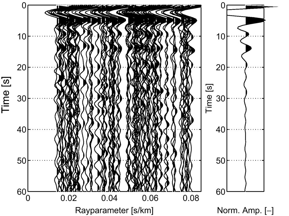
Visualization of the integrand (correlation panel, left) and sum (stack, right) of the seismic interferometric relation (Eq. (5)) for xA and xB both at station 413. The integrand is obtained by correlating noise records from the double frequency microseism.
Visualisation de l’intégrant (panneau de corrélation à gauche) et de la somme (panneau de sommation, à droite) de la relation sismique interférométrique (Éq. (5)) pour xA et xB, tous deux à la station 413. L’intégrant est obtenu par corrélation des enregistrements de bruit microsismique secondaire.
The largest features in Fig. 9(left), around t = 0, are the average autocorrelations of source-time functions of the noise (Sn(t), Eq. (3)) convolved with spikes at the time differences of the direct waves. The effective source-time functions of the noise are fairly consistent for the different rayparameters. They show a large drop in energy from t = 0 onwards until t≈7.5 s. At larger times the effective source-time functions are weaker and strongly varying, depending on the noise source, or mix of noise sources, that were active within a certain time window.
One other consistent feature can be observed in the correlation panel, with a negative phase at t≈11 s. This feature is mainly due to the correlation of the direct noise field with the free-surface reflected noise field as drawn in Fig. 6, and hence its negative phase.
The stack (the graph on the right-hand side in Fig. 9) may be interpreted as the reflection response as if there were a source and a receiver at station 413 (which station is located in the middle of subarray 1, Fig. 1). However, this stack is still imprinted by the limited illumination used and Sn(t). At later times, the stack shows a few other events, which were not readily interpretable in the correlation panel, but are likely to be subsurface reflections.
Similar stacks are obtained for all other station-combinations in subarray 1. The resolution is slightly increased by deconvolution with the stack of autocorrelations of the direct noise field. As a deconvolution trace, a time window between −7.5 and 7.5 s is selected from the zero-offset retrieval.
Fig. 10 a shows the resulting stacks of crosscorrelations of station 413 with all other stations in subarray 1. Hence, it is the estimation of the reflection response as if there were a source at station 413 and receivers at all other stations (such a panel is called a shotgather). The event with the largest amplitude could be interpreted as the direct field between the stations, if there was illumination from large rayparameters. Since we restricted the rayparameter band, this event between 0 and 7.5 s is an artifact. Fig. 10b shows the result after removing this artifact. It is compared with a synthetic reflection response (Fig. 10c). This synthetic response was obtained by forward modeling the wavefield due to a point source in the Cornell model for the crust in Northeast Africa (Seber et al., 1997), supplemented by the PREM model of the transition zone (Fig. 10d). The two main interfaces in this merged model are the Moho and Lehmann dicontinuities, at 34 and 217 km depth, respectively. The synthetic response (Fig. 10c) was convolved with a flipped Ricker wavelet to be consistent with the SI result (Fig. 10b).
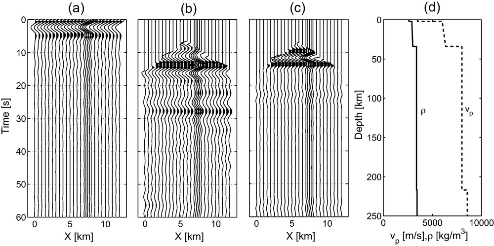
A retrieved shotgather for a virtual source at station 413 and receivers at all station locations of subarray 1 (Fig. 1), (a) before and (b) after muting the spurious event near t = 0, in comparison with (c) a synthetic shotgather for (d) a 1D Earth model for Northeast Africa.
Section pour une source virtuelle à la station 413 et capteurs sur toutes les autres localisations de stations du sous-réseau 1 (Fig. 1). (a) avant et (b) après élimination d’un évènement parasite près de t = 0, en comparaison avec (c) section pour (d) un modèle Earth 1D pour le Nord-Est de l’Afrique.
In the reference response (Fig. 10c) three reflections can be seen: at 11 s the Moho reflection, at 22 s the Moho multiple and at 57 s the Lehmann reflection. In the retrieved response (Fig. 10b), the same three reflections can be identified at similar times. Additionally, a few reflections were retrieved that were not forward modeled. The reflections at 17 and 34 s could be the primary and multiple, respectively, of the Hales discontinuity (Kind and Li, 2007). The reflection at 28 s has the right phase and timing to be the lithosphere-asthenophere-boundary (LAB) reflection. The amplitude is surprisingly large, though. Consequently, the reflection around 56 s could be explained by either a primary reflection from the Lehmann discontinuity or as a multiple from the LAB.
In Fig. 11, we show the retrieved shotgathers for a few other virtual source locations on subarray 1. Note the consistency for the different features for the different shotgathers.
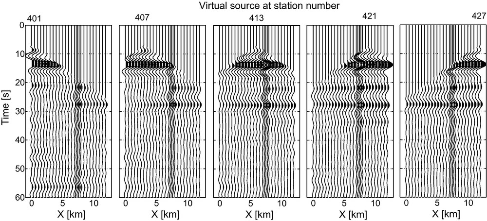
Retrieved shotgathers for, from left to right, a virtual source at station number 401, 407, 413, 421 and 427, respectively, and receivers on all other station locations of subarray 1 (Fig. 1).
Sections pour, de gauche à droite, une source virtuelle aux stations 401, 407, 413, 421, 427, respectivement et les capteurs sur toutes les autres positions de station du sous-réseau 1 (Fig. 1).
As a further processing, at all 110 stations (Fig. 1), we retrieved the zero-offset reflection response and picked the two-way traveltime of the Moho reflection. Fig. 12 depicts an interpolated image of these traveltimes. With the assumption that the Moho itself is flat, the traveltime anomalies in Fig. 12 can be interpreted as structure in the crust.
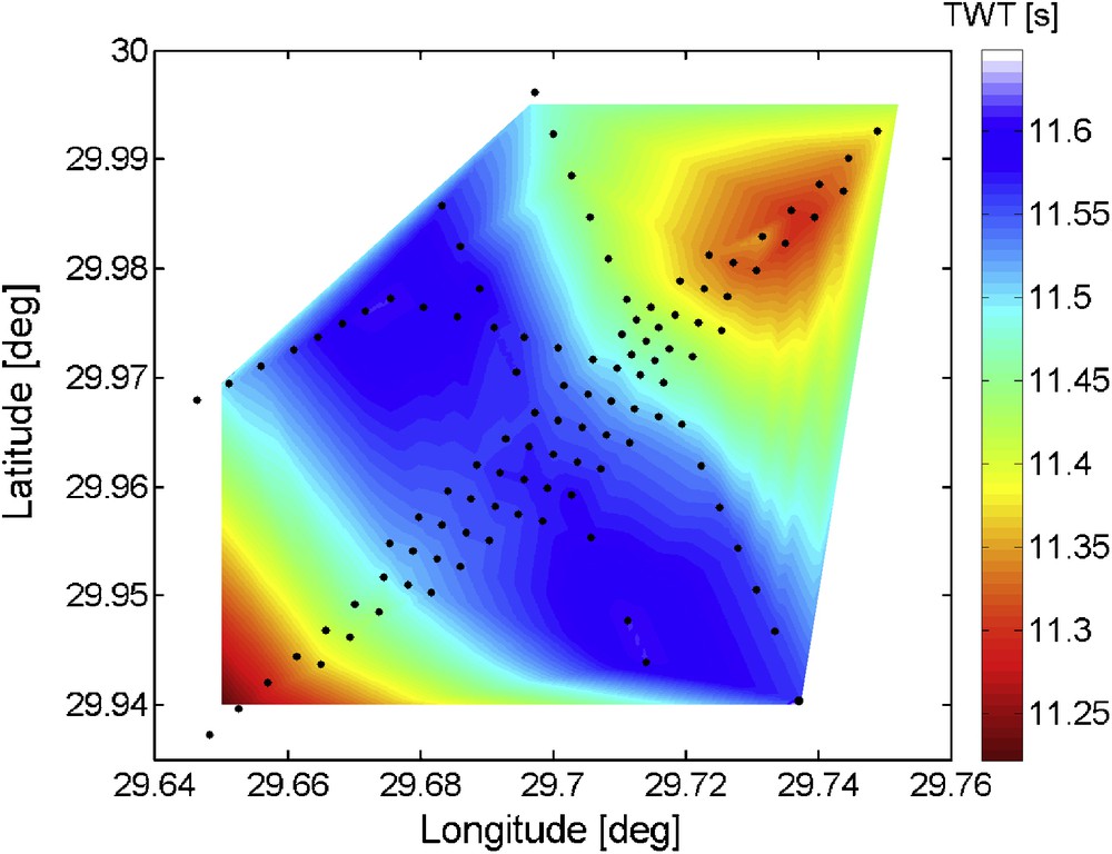
A 2D interpolation of the two-way traveltimes (TWT) of the retrieved Moho reflection (Fig. 10), at zero-offset. The station positions are depicted with black dots.
Interpolation 2D des temps de trajets doubles (TWT) de la réflexion de Moho extraite (Fig. 10), à déport 0. La position des stations est matérialisée par les points noirs.
6 MF band
We start the analysis of the recordings in the MF band ([0.4–1.0] Hz) by computing time-variation functions, as described in Section 5. The results are shown in Fig. 13. As for the DF band, we use 10-min records at station 402 for the PSD computations (Fig. 13a and b). In the MF band the noise sources tend to be of a shorter duration than in the SF and DF band. Hence, for the beamforming (Fig. 13c and d) we limit the time windows to 5 min.
MF-band noise-variation plots for 40 h of data, starting 12 October 2009 at 14:00. (a) Power spectrum density (PSD) variation on the Z-component and, for all components, (b) the averaged (over frequency) PSD variation, (c) the backazimuth and (d) the rayparameter variation.
Représentation de la variation de bruit dans la bande MF pour 40 h d’acquisition, débutant le 12 octobre 2009 à 14 h : (a) variation de la densité spectrale de puissance (PSD) sur la composante Z et, pour toutes les autres stations, (b) variation de PSD moyenne sur la bande de fréquence (c) azimuth en retour et (d) variation de paramètre du rai.
Only a small portion of the recorded energy is due to earthquake responses (Fig. 3). In Fig. 13a and b, these can be recognized as high-energy transient events. In the background of these transient peaks, we can notice a noise distribution which is relatively quiet between 0 and 17 h, which catches some energy related to the DF microseism between 17 and 30 h and which increases in strength between 30 and 40 h. The clear noise source in this later time-interval has a dominant frequency of about 0.6 Hz. Overall, there is more energy on the horizontal components (Fig. 13b). This hints at the presence of Love waves.
Fig. 13c shows the dominant backazimuth variation. Between 0 and 17 h, θdom(t) for the horizontal components (green and red lines) differs largely from the one for the vertical component (blue line). Hence, during this quiet time, the horizontal components pick up noise from a different source than the vertical component. From 17 h onwards the backazimuth estimations become identical for all components; all components detect predominantly noise from a source region WNW of the array.
Fig. 13d shows the dominant-rayparameter variation. A clear difference can be seen between the vertical component (blue line) and the horizontal components (green and red lines). The rayparameters estimated for the Z-component increase with time. For increasing time, these rayparameters can be explained by global, teleseismic and regional P-wave sources, respectively (Fig. 8). It appears that a P-wave source migrates towards the array. The rayparameters on the horizontal components are significantly larger and can be explained by a mix of crustal phases, Sg (p ≈ 0.31 s/km), Lg (p ≈ 0.28 s/km) and Sn (p ≈ 0.21 s/km) (Isacks and Stephens, 1975).
The rayparameter distribution estimated for the Z-component is favorable for body-wave SI processing. The further processing is almost identical to the one described for the DF band (Section 5).
From Figs. 1 and 5a we can infer that the azimuthal distribution of the sources is best suited for the retrieval of reflections below subarray 2. WNW of the Egypt array there is a good distribution of sources, both with respect to rayparameter and azimuth. Source locations on the ESE side are absent. Consequently, we have only one-sided illumination and we can use Eqs. (4) or (5).
We consider the 40 h of noise presented on Fig. 3 for all stations in subarray 2 and split up the records in time windows of 5 min duration. We leave out time windows with pdom larger than 0.08 s/km as were found through beamforming (Fig. 13d) to omit the necessity of a decomposition into P- and S-waves. Also we leave out time windows with pdom < 0.08 s/km, but with a notable surface-wave pollution. Consequently, from the 480 panels available, only 142 are used. Each panel is root-mean-square normalized. For each selected time window, all traces are mutually crosscorrelated. Subsequently, all crosscorrelations pertaining to the same station combination, are stacked. The resulting traces are ordered into shotgathers. For each shotgather, the imprint of Sn(t) (Eq. (3)) is mitigated by applying a source deconvolution. As a deconvolution trace, a time window between −3 and 3 s is selected from the virtual source trace, whose trace is the one obtained for xA and xB (Eq. (5)) both at the same station. Subsequently, the spurious event near t = 0 is muted. Finally, the retrieved responses are regularized to a station grid of 0.5 km to simplify the further processing.
Fig. 14 shows five reflection responses thus obtained. Until about 7 s, a few clear reflections can be recognized on all shotgathers. Notably, the primary reflection from the basement of the sedimentary basin at 3.1 s. After resorting the shotgathers to common-midpoint gathers, we estimate the average velocity of the basin to be 3.2 km/s. Hence, the basement can be found at about 5 km depth. From gravity data it was found that the basement depth of the Abu Gharadig depositional center varies between 6 and 12 km (Awad, 1985). Our Egypt array was located at the northeastern edge of this basin.
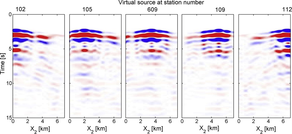
Retrieved shotgathers for, from left to right, a virtual source at station number 102, 105, 609, 110 and 112, respectively, and receivers on all other station locations of subarray 2 (Fig. 1). Blue and red denote positive and negative amplitudes, respectively.
Sections pour, de gauche à droite, une source virtuelle aux stations 102, 105, 609, 110 et 112 respectivement et les capteurs de toutes les autres localisations de stations du sous-réseau 2 (Fig. 1). Le bleu et le rouge dénotent respectivement les amplitudes positive et négative.
7 Discussion and conclusions
We analyzed 40 h of continuous data recorded by an array of three-component stations in Egypt. The purpose was to asses the applicability of body-wave SI.
We split up the noise in three distinct frequency bands (SF, DF and MF). For each band, we searched for the dominant noise sources by beamforming. The dominant noise sources turned out to be different for all considered bands.
The origins of the noise in the MF band seem to be largely unrelated to the DF microseism. This is consistent with the theory that the DF microseism is (indirectly) generated by swell, whereas higher frequencies are (indirectly) generated by local offshore winds (Kibblewhite and Ewans, 1985). In Zhang et al. (2009), the noise between 0.5 and 2.0 Hz showed a large correlation with regional offshore winds. For the Egypt array we did not compare the MF noise measurements with wind hindcasts. Still, between 17 and 40 h (Fig. 13), the rayparameters and backazimuths could be explained by regional and local winds in the eastern Mediterranean. Between 0 and 17 h, though, the detected rayparameters and backazimuths direct to sources in the North Atlantic and Pacific. Hence, it turns out that, with the absence of local or regional winds, also teleseismic (offshore-wind) noise sources are detectable in the MF band.
After beamforming the Z-component of the SF-band, it turned out that it was dominated by surface waves. Since it was our aim to retrieve body waves, we did not further process this band. For the DF and MF band, we split up the total noise record in small windows. We computed, for each time window and for each component, the PSD and the dominant rayparameter. Doing so, we could unravel the dominant wavemodes. For the DF and MF we found a dominance of P-waves on the Z-component and a mix of S-waves and surface waves on the other components.
Vinnik (1973) conjectured that P-waves would be the dominant wavemode at the Z-component, at epicentral distances of about 40 degrees from an oceanic source. At arrays far from offshore storms, surface waves induced by nearby storms would not mask the body-wave signal and hence primarily P-waves would be recorded. Our measurements in Egypt, which may be considered a shielded location for oceanic storms, supports his conjecture.
We found that considerable part of the Z-component noise panels in the DF and MF band was favorable for body-wave SI. The further processing of the noise records was very similar to the approach taken for transient records (Ruigrok et al., 2010). Only time windows with a favorable illumination and without surface-wave pollutions, were further processed. We did not discriminate between panels dominated by noise or by earthquake responses. However, the contribution of the earthquake responses was little, since each record was normalized and only a few panels were dominated by earthquake responses.
We retrieved P-wave reflection responses and delineated reflectors in the crust, the Moho and possibly the Hales and Lehmann discontinuity. The results from the two frequency bands, MF and DF, turned out to be well complimentary. With noise from the MF band we obtained reflections between two-way traveltime of about 2 and 7 s, while with DF noise we obtained reflections between 8 and 30 s and possibly even at later times. A longer noise registration would be necessary to find the reliability of possible transition-zone reflections. High-resolution reflection responses at shorter times can be obtained from noise at frequencies above 1 Hz, as was shown by Draganov et al. (2009).
The retrieved reflection responses could still be improved by better estimating the average autocorrelation of the noise (Sn(t), Eq. (3)). In this study we estimated Sn(t) by time-windowing stacked autocorrelations. This time window is truncated at the times we expect to see the first reflectivity. That is, at the time at which the gradual drop in energy from t = 0 onwards is broken by a local rise in energy. Though this might indeed indicate the time at which Sn(t) is not dominating anymore, Sn(t) has a much longer duration and might contain some notches at later times. To make a better estimation of Sn(t), the autocorrelation should be repeated for a few stations that are detecting the same noise field, but are installed on very different subsurfaces.
Thus far it has been shown that ocean-generated body-wave noise may be used for P-wave tomography (Roux et al., 2005; Zhang et al., 2010), for the retrieval of S-wave reflections (Zhan et al., 2010) and for the retrieval of P-wave reflections (this paper). How about receiver functions (Vinnik, 1977)? In principle, it is possible to use the same P-wave noise records for obtaining receiver functions. There are enough time windows with predominantly teleseismic P-waves arriving at the vertical component. Simultaneously though, the horizontal components pick up wavemodes with much higher rayparameters (Figs. 7d and 13d). The waves detected at the horizontal components are a mix of S-phases and surface waves. Hence, the challenge would be to clean out these wavemodes from the horizontal components, such that only P–S converted waves are left. Alternatively, for some arrays one might be lucky to find time windows not contaminated by other waves than P-S conversions.
A large amount of empirical microseism studies have appeared over the years (Koper et al., 2010). In addition, efforts are becoming increasingly successful for hindcasting microseismic sources. Based upon the theory by Longuet-Higgins (1950), Kedar et al. (2008) hindcasted pelagic microseismic Rayleigh-wave sources, using hindcasted ocean-wave data and bathymetry. The same modeling approach was used by Hillers et al. (2010) to identify deep-ocean regions with microseismic P-wave sources. Stutzmann et al. (2010) and Graham et al. (2010) included a model with reflection coefficients at the coasts to also hindcast microseismic sources near the continents. Hence, it becomes possible to assess where and when to measure to retrieve low-frequency P-wave reflection responses, now the microseismic (P-wave) source areas, and their yearly variations, are identified.
Compared to using earthquake records, the deployment time of arrays could be reduced if we use body-wave noise. With a favorable distribution of noise sources, a day to a week of noise recording would be sufficient, whereas a few months of array deployment would be needed to collect enough earthquake responses (Ruigrok et al., 2010).
Acknowledgements
This work is supported by The Netherlands Organization for Scientific Research NWO (grant Toptalent 2006 AB) and Shell International Exploration and Production B.V. We thank Shell Egypt NV for providing the data and for permission to publish the results. Furthermore, we would like to thank Kevin Ewans (Shell Metocean Department) for sharing his knowledge regarding microseisms and Deyan Draganov for proofreading the manuscript. Last but not least, we would like to thank two anonymous reviewers and Michel Campillo for their constructive comments.