


 CC-BY 4.0
1. Introduction
Enormous progress has been achieved in the modeling and understanding of the magnetic dynamo at work in the core of the Earth and other planets since the first 3D numerical simulations of Glatzmaier and Roberts [1995] and Kageyama et al. [1995]. It rapidly appeared that the magnetic fields produced by such numerical simulations met the main characteristics of the long-term magnetic field observed on Earth, such as its dipolarity, the presence of high-flux patches at high latitudes, and symmetry properties [Christensen et al. 1999, Olson and Christensen 2006, Christensen et al. 2010]. Magnetic intensity scaling laws for planetary and stellar dynamos were obtained by combining an analysis of the dominant terms of the governing equations with results of an extensive survey of numerical simulations [Christensen and Aubert 2006, Christensen 2010].
In the meantime, shorter timescale manifestations of the geodynamo were unveiled, such as a large-scale off-centered anticyclone [e.g., Pais and Jault 2008], and torsional waves (geostrophic Alfvén waves) with periods of a few years [Gillet et al. 2010]. These new observations prompted efforts to run numerical simulations at more extreme parameter values [Schaeffer et al. 2017, Aubert et al. 2017, Aubert 2023], increasing the role of rotation by decreasing the Ekman number down to Ek = 10−7, and increasing the convective forcing up to Ra∕Rac = 6300, where Ra is the Rayleigh number, and Rac its critical value. These extreme simulations of the geodynamo successfully account for fast dynamics retrieved from observations.
In view of this remarkable progress, it might seem that most problems are solved. In fact, hot debates are still roaming on several crucial issues. One of them concerns the dominant length-scale of convective structures in Earth’s core. Column widths of 100 m are suggested by Yan and Calkins [2022] while Guervilly et al. [2019] advocate 30 km. Extrapolating force-balances from numerical simulations and laboratory experiments to natural systems is another issue [Aurnou and King 2017, Schwaiger et al. 2019, Teed and Dormy 2023]. The relevance of scenarios with weak and strong magnetic field branches is also hotly debated [Dormy 2016]. One extreme viewpoint being expressed by Cattaneo and Hughes [2022] who claim that Earth would not have been able to produce a magnetic field as strong as today without Moon’s help.
There is room for such diverging views because the distance from numerically accessible parameters to expected planetary values remains vertiginous. Laboratory experiments somewhat enlarge the accessible range but are limited to non-dynamo regimes, making the link with numerics and observations difficult.
This is the motivation for exploring a different route: instead of extrapolating available simulations to core conditions, start from the actual expected properties of the core, and patch scenarios of turbulence that correspond to different regimes encountered at different scales. This leads to the construction of 𝜏–ℓ regime diagrams of turbulence, as briefly introduced by Nataf and Schaeffer [2015].
Our experience is that this approach is an excellent intuition-booster. It provides a simple graphical support that can greatly help deciphering and testing more mathematically-motivated approaches. However, we observe that it has not yet received an audience, perhaps because it clearly advocates a “fuzzy physics” method, and also because it was originally published in a limited-access collection.
In this article, we present a largely renewed and extended version of the 𝜏–ℓ regime diagrams we originally proposed. We detail the steps for constructing such diagrams, providing examples of application to numerical simulations and laboratory experiments. Key properties of 𝜏–ℓ diagrams are highlighted and illustrated by simple examples.
The central part of the article is devoted to an application to the Earth’s core. We propose scenarios for a non-magnetic rotating convective core, and for a dynamo-generating rotating convective core. The resulting diagrams are compared with the predictions of several scaling analyses [Christensen and Aubert 2006, Christensen 2010, Davidson 2013, Aubert et al. 2017].
Nataf and Schaeffer [2015] were building scenarios from the observed large-scale flow and magnetic field, and testing how they were compatible with the expected available power. In this article, our 𝜏–ℓ diagrams are constructed to satisfy a given constraint on the convective or dissipated power, a key property of turbulent flows. Comparison with the observed flow and magnetic field (when available) is used as a validation test. This is a more challenging exercise, which leads us to consider the various force balances that could govern the dynamics of the object. We derive the 𝜏–ℓ translation of the main relevant force balances (CIA, QG-CIA, MAC, QG-MAC, IMAC). It turns out that these translations and their graphical representations are very telling.
This should facilitate the construction of 𝜏–ℓ diagrams for planets, exoplanets and stars for which no direct observation of the large-scale flow velocity and magnetic field is available. Indeed, planets are thermal machines and their thermal evolution is probably what we can estimate best. Liquid cores of planets cool down on geological timescales, generating convective motions. Convective power, which can be estimated from the planet’s thermal history [e.g., Stevenson et al. 1983, Lister 2003, Nimmo 2015, Landeau et al. 2022, Driscoll and Davies 2023], sustains fluid flow and magnetic field. Dissipation of this power by either momentum or magnetic diffusion, or both, controls the regimes of turbulence the system experiences.
We present and illustrate the construction rules and key properties of 𝜏–ℓ regime diagrams of turbulence in Section 2. Section 3 introduces the physical phenomena at work in planetary cores, and relates 𝜏–ℓ diagrams to classical dimensionless numbers. Section 4 presents 𝜏–ℓ regime diagrams for a non-magnetic rotating core. 𝜏–ℓ diagrams of the present-day geodynamo are built in Section 5. Both sections emphasize the crucial role of the available convective power and force balances. The discussion Section 6 illustrates how 𝜏–ℓ diagrams bring a new light on several ongoing debates. Limitations and perspectives are outlined in Section 7, and we conclude in Section 8. Appendix A provides rules for converting spectra into 𝜏–ℓ language. Simple Python programs used to build 𝜏–ℓ diagrams are given as supplementary material, together with examples from numerical simulations and laboratory experiments.
2. Construction rules and key properties of 𝜏–ℓ diagrams
This section presents the rules used to construct 𝜏–ℓ diagrams. Turbulent systems display a wide range of length-scales and timescales. Timescales of physical phenomena such as diffusion or wave propagation depend upon the length-scale at which they operate. For example, timescale 𝜏𝜈 of momentum diffusion at length-scale ℓ can be written as 𝜏𝜈(ℓ) = ℓ2∕𝜈, where 𝜈 is the kinematic viscosity. Similarly, turnover time 𝜏u of a vortex of radius ℓ is given by 𝜏u(ℓ) = ℓ∕u(ℓ), where u(ℓ) is the vortex fluid velocity. We build 𝜏–ℓ regime diagrams by plotting timescales 𝜏x as a function of length-scale ℓ in a log–log plot, for all the different physical phenomena x that govern the fluid flow in a given system.
Construction rules of 𝜏–ℓ regime diagrams
𝜏–ℓ regime diagrams are “object-oriented”. They are built following these steps:
- Identify physical phenomena that play an important role in the object under study.
- Document relevant physical properties (viscosity, thermal diffusivity, rotation rate, etc).
- Build and draw lines 𝜏(ℓ) that control dissipative and wave propagation phenomena.
- Identify different turbulence regimes the object might experience.
- Construct and draw lines 𝜏(ℓ) of fields (velocity, buoyancy, magnetic field) that describe the object’s turbulent behaviour, given a dissipated power .
- Compare predictions with observables such as large-scale flow velocity and magnetic field, when available.
2.1. A simple example: Kolmogorov’s universal turbulence
We first illustrate the construction rules of 𝜏–ℓ diagrams with the simple example of Kolmogorov’s universal turbulence [Kolmogorov 1941]. Although this is not the kind of turbulence we expect in planetary cores, we pick a range of length-scales and timescales typical of the Earth core. Figure 1 is a log–log plot of timescales spanning a range from 10 s to 32,000 years versus length-scales from 1 cm to Ro = 3480 km, the radius of the core.
𝜏–ℓ regime diagram for Kolmogorov’s universal turbulence [Kolmogorov 1941]. Teal line labeled 𝜈 is viscous dissipation line 𝜏𝜈(ℓ) = ℓ2∕𝜈. The thick blue line is eddy turnover time 𝜏u(ℓ) =𝜖 −1∕3 ℓ2∕3 inferred from Kolmogorov’s law, assuming that energy is injected at core radius length-scale ℓ = Ro. These two lines intersect where the ℓ-scale Reynolds number ℜ(ℓ) ∼ 1, as marked by a circle. Total energy dissipation rate can be read at this intersection (blue arrow), using square markers drawn and labelled along the viscous line. Markers are a factor of 103 apart, the 1 TW marker being filled.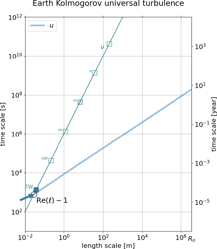
2.1.1. 𝜏𝜈(ℓ) line
We pick a viscosity value 𝜈 = 10−6⋅m2⋅s−1 and draw the 𝜏𝜈(ℓ) viscous dissipation line:
| (1) |
2.1.2. 𝜏u(ℓ) line
In Kolmogorov’s universal turbulence, kinetic energy cascades down from large length-scales to small scales, from the energy injection scale down to the viscous dissipation scale. The range in between is called the inertial range. The kinetic energy density spectrum E(k) in the inertial range obeys Kolmogorov’s law:
| (2) |
To build line 𝜏u(ℓ), we need to convert kinetic energy density into velocity. It is common to define an “eddy turnover time” as 𝜏u(ℓ) = ℓ∕u(ℓ), with u2(ℓ) ∼ E(k)k and ℓ ∼ 1∕k (see Appendix A.1). This translates into:
| (3) |
| (4) |
We draw this 𝜏u(ℓ) line in Figure 1, assuming that the energy injection length-scale is Ro, and choosing an injection timescale, which will be discussed later.
2.1.3. ℓ-scale Reynolds number
We terminate line 𝜏u(ℓ) where it hits viscous line 𝜏𝜈(ℓ). This intersection yields Kolmogorov microscales (ℓK,𝜏K), for which , i.e., u(ℓK)ℓK∕𝜈 = 1. Defining an ℓ-scale Reynolds number ℜ(ℓ) = u(ℓ)ℓ∕𝜈, we note that the intersection of the eddy turnover time line 𝜏u(ℓ) with the viscous line 𝜏𝜈(ℓ) occurs at ℜ(ℓ) = 1. It marks the transition from the inertial cascade at large scale to the viscous dissipation regime at small scale.
2.1.4. Power dissipation markers
In Kolmogorov’s theory, the energy injected at large scale cascades down with no loss to small scales at which viscous dissipation takes place. This dissipation range starts at the intersection of lines 𝜏u and 𝜏𝜈, where R e(ℓ) ∼ 1, which defines Kolmogorov microscales (ℓK,𝜏K). From Equations (1) and (4), we deduce:
| (5) |
2.1.5. Energy
In Kolmogorov’s universal turbulence, kinetic energy is dominated by large length-scales. In 𝜏–ℓ diagrams, we retrieve kinetic energy from the square of the inverse of 𝜏u(Ro) since:
| (6) |
Key properties of 𝜏–ℓregime diagrams
- 𝜏–ℓ regime diagrams gather in a simple graphical representation many of the ingredients that control the dynamics of a turbulent fluid system.
- In 𝜏–ℓ regime diagrams, intersections of lines 𝜏x(ℓ) and 𝜏y(ℓ) of physical phenomena x and y occur where ℓ-scale dimensionless number Z(ℓ) = 𝜏y(ℓ)∕𝜏x(ℓ) equals 1. They mark a change in the system’s dynamical regime.
- Usual integral-scale values of dimensionless numbers are obtained from the ratio of relevant 𝜏x(ℓ) and 𝜏y(ℓ) times at integral scale ℓ = Ro.
- Total dissipated power can be marked along 𝜏(ℓ) lines of dissipative phenomena.
- Energies of different types (kinetic, gravitational, magnetic) are represented by the inverse square of corresponding 𝜏(Ro).
- 𝜏–ℓ regime diagrams are a useful tool to infer or test turbulence scenarios. They are not a theory of turbulence.
3. Physical phenomena in planetary cores and dimensionless numbers
We now turn our attention to planetary cores. Flow within planetary cores are mostly powered by thermal or thermo-compositional convection. They often produce a magnetic field. Most importantly, these flows occur in a rotating spherical system.
In this section, we introduce the 𝜏–ℓ lines these physical phenomena contribute. We illustrate the resulting 𝜏–ℓ regime diagram template, using values pertaining to Earth’s core, and relate the diagram to various dimensionless numbers used to characterize planetary core dynamics.
3.1. Physical phenomena and their 𝜏–ℓ expressions
Table 1 gives the expressions of major 𝜏(ℓ) times pertaining to planetary cores. 𝜏𝜈(ℓ) and 𝜏u(ℓ) times have been introduced in Section 2.1. Convection adds thermal diffusion and buoyancy scales. Rotation, spherical boundaries, and magnetic field contribute key additional timescales.
Notation and expression of 𝜏(ℓ) times of relevant physical phenomena for planetary cores
| Time | Expression | Phenomenon |
|---|---|---|
| 𝜏𝜈(ℓ) | ℓ2∕𝜈 | Viscous dissipation |
| 𝜏𝜅(ℓ) | ℓ2∕𝜅 | Thermal diffusion |
| 𝜏𝜒(ℓ) | ℓ2∕𝜒 | Compositional diffusion |
| 𝜏𝜂(ℓ) | ℓ2∕𝜂 | Magnetic dissipation |
| t𝛺 | 1∕𝛺 | Rotation |
| 𝜏Rossby(ℓ) | Ro∕𝛺ℓ | Rossby wave propagation |
| 𝜏Alfven(ℓ) | Alfvén wave propagation | |
| 𝜏𝜌(ℓ) | Buoyancy (or free-fall) | |
| 𝜏u(ℓ) | ℓ∕u(ℓ) | Eddy turnover |
| 𝜏b(ℓ) | Alfvén wave collision |
Fluid properties: density 𝜌; kinematic viscosity 𝜈; thermal and compositional diffusivities 𝜅 and 𝜒, respectively; magnetic diffusivity 𝜂; magnetic permeability 𝜇. System properties: radius Ro; gravity g; rotation rate 𝛺; large-scale magnetic field B0. Turbulent flow properties: 𝛥𝜌(ℓ), u(ℓ) and b(ℓ) are ℓ-scale density anomaly, flow velocity, and magnetic field intensity, respectively. We also write 𝜏𝜂(Ro) as T𝜂 for short. Adapted from Table 1 of Chapter 8.06 of Treatise on Geophysics [Nataf and Schaeffer 2015] with permission.
We discuss the origin and meaning of these various 𝜏(ℓ) scales, and illustrate the 𝜏–ℓ template they provide in Earth’s core example (Figure 2), using its properties presented in Section 3.3. We first ignore the magnetic field and build the template of Figure 2a.
𝜏–ℓ regime diagram templates for the Earth’s core. The time-length relationships of relevant physical phenomena, as given in Table 1, are drawn in a log–log plot of timescale versus length-scale, using Earth core values from Table 3 presented in Section 3.3. (a) Template ignoring the magnetic field. The steep solid lines labeled 𝜒, 𝜈 and 𝜅 are diffusion times 𝜏𝜒(ℓ), 𝜏𝜈(ℓ), and 𝜏𝜅(ℓ), respectively. The dash–dot horizontal line is the rotation time t𝛺. The Rossby line 𝜏Rossby(ℓ) is drawn as a wavy line pinned to t𝛺. Markers along lines 𝜏𝜈(ℓ) and 𝜏Rossby(ℓ) indicate viscous power dissipation. Markers are a factor of 1000 apart, the 1 TW marker being filled. The circle labeled Ek at the intersection of the viscous 𝜏𝜈(ℓ) and t𝛺 lines mark the length-scale at which the ℓ-scale Ekman number equals 1. Same thing for the thermal Ekman number Ek𝜅(ℓ). (b) Template including the magnetic field. Same as (a) with additional lines and labels brought by the magnetic field. The steep solid red line labeled 𝜂 is the magnetic diffusion line 𝜏𝜂(ℓ). Markers along that line indicate Ohmic power dissipation. Markers are a factor of 1000 apart, the 1 TW marker being filled. The Alfvén line 𝜏Alfven(ℓ) is drawn as a wavy line pinned to the observed large-scale magnetic field Alfvén time . Circles labeled Ek𝜂, Lu and 𝜆 at line intersections mark scales at which the corresponding ℓ-scale dimensionless number (see Table 2) equals 1. See Sections 3.1.6 and 3.3 for more information.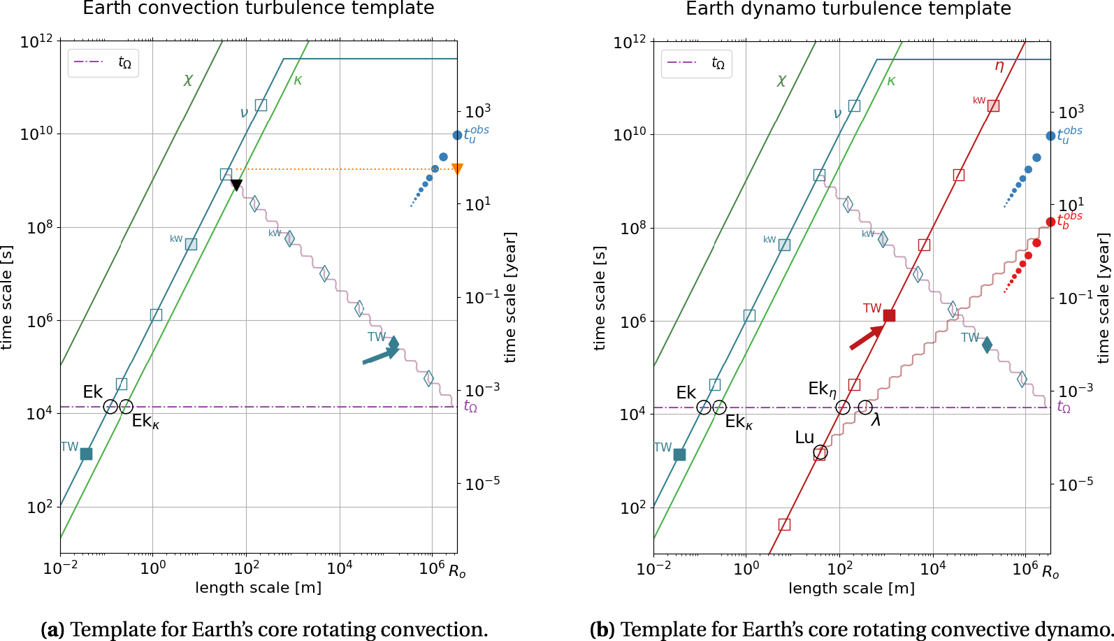
3.1.1. Diffusion
Lines labeled 𝜈, 𝜅 and 𝜒 are diffusion 𝜏–ℓ lines. Timescales of diffusive phenomena all share the same form 𝜏(ℓ) = ℓ2∕D, where diffusivity D is 𝜈, 𝜅 or 𝜒 depending upon which field diffuses: momentum, temperature, or composition, respectively.
3.1.2. Convection
We introduce a “buoyancy” or “free-fall” timescale , which is the time it takes for a parcel of fluid with density anomaly 𝛥𝜌(ℓ) to rise or sink a distance ℓ in the absence of diffusion. 𝜏𝜌(ℓ) relates to density anomaly 𝛥𝜌 at length-scale ℓ. Density anomaly, flow velocity and magnetic field constitute the three fields for which we seek an adequate turbulent description.
We have shown in Section 2.1 that the value of 𝜏u at integral scale Ro measures the kinetic energy of the flow. Similarly, gravitational energy is measured by 𝜏𝜌(Ro) (as long as the slope of 𝜏𝜌(ℓ) is less than 3∕2) since:
| (7) |
3.1.3. Rotation
Rotation is a crucial ingredient of planetary core dynamics. It adds one important time in our 𝜏–ℓ regime diagram: the rotation time t𝛺 =𝛺 −1, i.e., one day divided by 2π. Physical phenomena operating at timescales smaller than t𝛺 are not influenced by planet’s spin, while those with longer timescales feel the effect of rotation. We thus draw a horizontal line at t𝛺 in the diagram of Figure 2a. The intersection of this line with the viscous line yields Ekman layer’s thickness . Viscous forces are balanced by Coriolis acceleration in these thin Ekman layers. ℓE is the only length-scale one can build from 𝜈 and 𝛺 alone, and it controls friction, hence viscous dissipation, that takes place at boundaries. It turns out that boundaries bring up new important dynamical constraints and scales.
3.1.4. Rotation and spherical boundaries
We will not review here the vast literature on rotating fluids in containers. The book of Greenspan [1968] remains amazingly central. At this stage, let us simply recall that Navier–Stokes equation reduces to geostrophic equilibrium when Coriolis acceleration dominates:
| (8) |
| (9) |
Proudman–Taylor constraint would inhibit all fluid motions in a rotating fluid bounded by a solid container. Accounting for the presence of a thin Ekman layer that accommodates a velocity jump between the fluid bulk and the boundary, geostrophic flows are allowed, which follow contours of equal fluid column-height (measured in the z-direction), i.e., azimuthal flows in a spherical container. In most situations, Quasi-geostrophic (QG) fluid motions are also observed, which approximately satisfy Proudman–Taylor constraint (i.e., z-invariance) in the bulk (at least for one component, typically the azimuthal velocity).
It is important to note that Proudman–Taylor constraint is established by the propagation of inertial waves in the fluid, and is effective only when they had time to reach a boundary. Thus, a localized eddy of radius ℓ grows into a columnar vortex at a speed equal to 𝛺ℓ [Davidson et al. 2006]. This means that large eddies rapidly form quasi-geostrophic columns, while it takes more time for small eddies to form core-size columns. Time for reaching quasi-geostrophy is thus given by:
| (10) |
Note that 𝜏Rossby(ℓ) also equals the time it takes for a Rossby wave of wavelength ℓ to propagate one wavelength (hence its name) [Nataf and Schaeffer 2015]. The intersection of the 𝜏u(ℓ) line with the Rossby line has , which defines a Rhines scale (originally more precisely defined as in a thin shell, where 𝛽 = 2𝛺sin𝜃∕Ro is the northward gradient of Coriolis frequency at colatitude 𝜃 [Rhines 1975], here extended to a wide gap [Busse 1970, Schopp and Colin de Verdière 1997]).
Flow is quasi-geostrophic for scales above line 𝜏Rossby(ℓ). In the triangle formed by the Rossby line, the viscous line and line t𝛺, flow structures are elongated parallel to the spin axis but not enough to reach both boundaries. Flow is 3D beneath line t𝛺.
3.1.5. Quasi-geostrophic dissipation
Quasi-geostrophic vortices dissipate kinetic energy by Ekman friction at no-slip boundaries of the liquid core. We approximate energy loss rate pℓ of a single QG vortex of radius ℓ by:
| (11) |
| (12) |
| (13) |
Going back to the viscous line 𝜏𝜈(ℓ), we terminate it at the spin-up time years, which is the time it takes for a change in the outer boundary spinning rate to be transmitted to the entire volume of the core.
3.1.6. A note on convection onset
We can already illustrate an interesting insight provided by this simple 𝜏–ℓ template, by adding the scales appearing at the onset of convection in this rotating spherical system. This topic has a long history, starting with the pioneer studies of Roberts [1968] and Busse [1970], followed by Jones et al. [2000], Dormy et al. [2004], Zhang et al. [2007]. It is found that convection sets in as a travelling thermal Rossby wave, forming columns aligned with the spin axis, whose width is controlled by viscosity in the bulk of the spherical shell. A 𝜏–ℓ translation of the length-scale, period, and Rayleigh number at convection onset is given in Appendix B.
In Figure 2a, a black triangle marks the length-scale and period at convection onset. It lies at the intersection of the Rossby and thermal diffusion lines, close to the viscous diffusion line, as expected for a viscously-controlled quasi-geostrophic thermal Rossby wave. We read a column-width of about 100 m. Is this the typical convective length-scale in the Earth’s core? We will get back to this question in Section 6.3. The orange triangle at ℓ = Ro marks the critical free-fall time deduced from the critical Rayleigh number (see Appendix B).
3.1.7. Magnetic field, magnetic dissipation, magnetic energy
Magnetic fields are often produced and sustained by dynamo action within planetary cores. We now add the magnetic field to build the template of Figure 2b. The red line labeled 𝜂 is the magnetic diffusion line 𝜏𝜂(ℓ). Magnetic dissipation markers are labeled along that line, following the same rule as in Equation (5).
The presence of a magnetic field allows the propagation of magnetohydrodynamic waves called Alfvén waves [Alfvén 1942]. In a uniform magnetic field B0, these waves propagate at speed , where 𝜇 is fluid’s magnetic permeability. Assuming a large-scale magnetic field B0, we construct line , the time it takes for an Alfvén wave to propagate over a distance ℓ. It is drawn as a red wavy line in Figure 2b.
To describe the magnetic field in the system, we define a similar timescale, replacing B0 by ℓ-scale magnetic field b(ℓ). Note that 𝜏b(Ro) =𝜏 Alfven(Ro) provides the magnitude of magnetic energy (as long as the slope of 𝜏b(ℓ) is less than 3∕2), since:
| (14) |
3.2. Dimensionless numbers
In order to connect to the huge literature pertaining to geophysical and astrophysical fluid dynamics, it is important to relate our 𝜏–ℓ regime diagrams to widely used dimensionless numbers. Dimensionless numbers provide the minimum number of parameters needed to describe a physical system. They permit a comparison of widely different systems that yield the same dimensionless numbers. These numbers are dimensionless combinations of properties and field variables that appear when the equations governing the dynamics of the system under study are made dimensionless by normalizing their various terms by “typical scales”.
For example, Reynolds number for a system of size L will be written: ℜ = U L∕𝜈, where U is a typical fluid velocity, and 𝜈 kinematic viscosity. Usually, it is when this dimensionless number is of order 1 that a change of regime occurs. In this example: a change between a regime where momentum diffusion dominates over advection when ℜ < 1 to one where advection dominates for ℜ > 1.
Most dimensionless numbers can be written as the ratio of two times. In our approach, we define length-scale dependent dimensionless numbers, constructed as the ratios of the timescales of the relevant physical phenomena at that length-scale. We thus define ℓ-scale Reynolds number as: ℜ(ℓ) =𝜏 𝜈(ℓ)∕𝜏u(ℓ), where 𝜏𝜈(ℓ) is momentum diffusion timescale at length-scale ℓ, while 𝜏u(ℓ) is the overturn time of a vortex of radius ℓ. Table 2 gives the expressions of ℓ-scale dimensionless numbers pertaining to planetary liquid core dynamics.
Expressions of ℓ-scale dimensionless numbers
| Number | Expression | Time ratio | Name |
|---|---|---|---|
| ℜ(ℓ) | Reynolds | ||
| Ra(ℓ) | Rayleigh | ||
| Ek(ℓ) | Ekman | ||
| Ek𝜅(ℓ) | Thermal Ekman | ||
| Ek𝜂(ℓ) | Magnetic Ekman | ||
| Ro(ℓ) | Rossby | ||
| Roff(ℓ) | Free-fall Rossby | ||
| Rm(ℓ) | Magnetic Reynolds | ||
| Lu(ℓ) | Lundquist | ||
| 𝛬d(ℓ) | Dynamical Elsasser | ||
| 𝜆(ℓ) | Lehnert |
These numbers are also expressed as ratios of characteristic ℓ-scale times, which are defined in Table 1. One recovers the classical expression of these numbers at integral scale by setting ℓ = Ro. Adapted from Table 2 of Chapter 8.06 of Treatise on Geophysics [Nataf and Schaeffer 2015] with permission.
In 𝜏–ℓ regime diagrams, the intersection of the 𝜏x(ℓ) and 𝜏y(ℓ) lines of physical phenomena x and y occurs where ℓ-scale dimensionless number Z(ℓ) =𝜏 y(ℓ)∕𝜏x(ℓ) equals 1. Each such intersection marks a change in the system’s dynamic regime.
In Figures 2a and 2b, we have labeled several line intersections, where specific dimensionless numbers equal 1. The intersections of line t𝛺 and the 𝜈, 𝜅 and 𝜂 lines indicate where corresponding ℓ-scale Ekman numbers equal 1 in the 𝜏–ℓ plane. The intersection of the Alfvén and magnetic diffusion lines defines where the ℓ-scale Lundquist number equals 1, marking a change from propagating Alfvén waves at larger scales to damped waves at smaller scales. Similarly, the intersection of the Alfvén and t𝛺 lines yields 𝜆(ℓ) ∼ 1, where 𝜆 is the Lehnert number [Lehnert 1954, Jault 2008]. System rotation favors quasi-geostrophic Alfvén waves at timescales above this intersection.
More dimensionless numbers, such as ℜ, Rm, Ra, Ro, Roff, and 𝛬d, will appear when we plot lines 𝜏𝜌(ℓ), 𝜏u(ℓ) and 𝜏b(ℓ) of the system’s density, velocity and magnetic fields for the different turbulence scenarios we will explore.
3.3. A word on Earth’s core properties
Core properties used to build the 𝜏–ℓ diagrams of Figure 2 are listed in Table 3. Most are taken from Peter Olson’s review in Treatise on Geophysics [Olson 2015]. Some of them are known with great precision (to about 1‰ for core radius Ro and liquid core mass Mo), but others are poorly constrained (to about 1 or 2 orders of magnitude for viscosity 𝜈 and compositional diffusivity 𝜒). In addition, most physical properties are expected to vary with radius. None of these (important) subtleties are taken into account in the “fuzzy” approach we advocate for building 𝜏–ℓ regime diagrams. Note that we systematically drop all numerical prefactors, including 2π.
Properties of Earth’s core
| Symbol | Value | Unit | Property |
|---|---|---|---|
| 𝜈 | 10−6 | m2⋅s−1 | Kinematic viscosity |
| 𝜅 | 5 × 10⁻⁶ | m2⋅s−1 | Thermal diffusivity |
| 𝜒 | 10−9 | m2⋅s−1 | Compositional diffusivity |
| 𝜂 | 1 | m2⋅s−1 | Magnetic diffusivity |
| 𝜌 | 10.9 × 10³ | kg⋅m−3 | Density |
| 𝛼 | 1.2 × 10⁻⁵ | K−1 | Thermal expansion coefficient |
| CP | 850 | J⋅kg−1⋅K−1 | Specific heat capacity |
| Ro | 3.48 × 10⁶ | m | Core radius |
| Ri | 1.22 × 10⁶ | m | Inner core radius |
| Mo | 1.835 × 1024 | kg | Outer core mass |
| g | 8 | m⋅s−2 | Gravity |
| t𝛺 | 1.38 × 10⁴ | s | Earth’s rotation time (i.e. 1∕2π day) |
| 3 × 10¹² | W | Available convective power | |
| 9 × 10⁹ | s | Ro-scale core flow time (i.e. ≃300 years) | |
| 1.4 × 10⁸ | s | Ro-scale Alfvén wave time (i.e. ≃4 years) |
As noted in Section 1, the power available to drive the dynamics of the system under study is a key ingredient. It largely controls the different turbulence regimes the system will experience. Thermal evolution of the Earth has received considerable attention (see Nimmo [2015], Landeau et al. [2022], Driscoll and Davies [2023] for reviews). It is now well established that the dynamics of Earth’s core today is powered by its slow cooling, enhanced by the resulting growth of the solid inner core. As iron-nickel alloy crystallizes at its surface, it releases latent heat and light elements that drive convection and power the geodynamo.
Despite uncertainties on isentropic heat flux, the available convective power is found to be in the range 0.8–5 × 10¹² W for present-day core [Nimmo 2015, Landeau et al. 2022]. We adopt value TW. This value is pointed by a blue arrow on the Rossby line in Figure 2a, and by a red arrow on the magnetic dissipation line in Figure 2b.
The last two rows in Table 3 are not used to build 𝜏–ℓ diagrams, but instead to test their relevance. Large-scale vortex turnover time years is retrieved from core flow inversions of magnetic secular variation [e.g., Pais and Jault 2008]. Large-scale Alfvén wave propagation time years is deduced from the discovery and analysis of “torsional oscillations” in Earth’s core [Gillet et al. 2010].
It is also observed that the Lowes–Mauersberger spectrum of magnetic energy is flat at the core-mantle boundary up to harmonic degree 10 [e.g., Langlais et al. 2014]. This means that energy is independent of length-scale in this scale-range, which translates into a 𝜏b(ℓ) ∝ ℓ3∕2 trend at large-scale (see Appendix A.2.1). Similarly, core flow inversions favor an almost flat harmonic spectrum of kinetic energy up to degree 10 [Roberts and King 2013, Aubert 2013, Gillet et al. 2015, Baerenzung et al. 2016]. These trends are sketched by colored disks labeled and in Figure 2.
4. 𝜏–ℓ regime diagrams for a non-magnetic rotating convective core
Building a turbulence scenario for a given system, starting from the power it dissipates, requires estimating the balance of forces at different length-scales. We thus start by expressing the 𝜏–ℓ translation of expected relevant force balances. We then focus on a quasi-geostrophic regime, which we illustrate with the 𝜏–ℓ diagram of an actual numerical simulation. We then propose an idealized scenario of turbulent convection in Earth’s core in the absence of a magnetic field.
4.1. 𝜏–ℓ expression of force balances in rotating convection
Let us start from the Navier–Stokes equation for deviations from hydrostatic equilibrium in an incompressible fluid under the Boussinesq approximation:
| (15) |
We already recalled in Section 3.1.4 that Equation (15) reduces to geostrophic equilibrium (8) when Coriolis acceleration strongly dominates, yielding Proudman–Taylor constraint (9). However, this equation is a diagnostic equation that can’t be used on its own, as gets clear when Equation (15) is curled to obtain the vorticity equation (see Jones [2015] for a more complete treatment). Reintroducing other accelerations and forces in the vorticity equation can lead to two different situations: (i) Proudman–Taylor constraint is broken and we get a three-term balance between Coriolis, inertia (or viscosity) and buoyancy; (ii) Coriolis acceleration is still dominant, and flow is quasi-geostrophic at leading order, with a small velocity gradient along the spin axis (𝜴⋅𝛻)u, scaling as 1∕ℓ∥, where ℓ∥∼ Ro [Julien et al. 2012].
4.1.1. Coriolis-Inertia-Archimedes (CIA)
Let’s first consider the first situation, with a three-term balance of Coriolis, inertia and Archimedean forces. At a given length-scale ℓ𝛺, retaining these forces in the curl of Equation (15) yields:
| (16) |
| (17) |
| (18) |
4.1.2. Quasi-geostrophic Coriolis-Inertia-Archimedes (QG-CIA)
The second situation is more relevant for the Earth’s core in the absence of a magnetic field. We still consider a three-term balance of Coriolis, inertia and Archimedean forces, but in which the Coriolis term is reduced to its ageostrophic part:
| (19) |
Translating in 𝜏–ℓ language, and assuming ℓ∥∼ Ro, we get:
| (20) |
| (21) |
4.2. 𝜏–ℓ diagram of a remarkable numerical simulation
We focus here on rapid rotation regimes (small Rossby number), for which the leading order balance is quasi-geostrophic. Important results have been obtained for this regime by Guervilly et al. [2019], who performed numerical simulations of thermal convection at low Prandtl number (Pr = 10−2 and 10−1) in a sphere, at Ekman numbers down to Ek(Ro) = 10−8 in 3D, and to Ek(Ro) = 10−11 in quasi-geostrophic 2D. In this section, we build the 𝜏–ℓ diagram of their most extreme 3D simulation, at Ek(Ro) = 10−8and Pr = 10−2, and discuss its implications. Figure 3a displays the 𝜏–ℓ diagram we obtain.
𝜏–ℓ diagrams for non-magnetic rapidly rotating convection. Refer to Figure 2a and Section 3 for a complete description of the background “template”. (a) 3D numerical simulation from Guervilly et al. [2019]. Field variables u and 𝜌 of the simulation are represented by blue 𝜏u(ℓ) and orange 𝜏𝜌(ℓ) lines, respectively, which are 𝜏–ℓ translations of their respective volume-averaged order m-spectra (see Appendix A.2.3). Simulation’s viscous dissipation in the bulk can be read on line 𝜏𝜈(ℓ) at the blue arrow, while viscous dissipation in Ekman layers is marked by a blue arrow on the Rossby line. Additional pale blue line labeled ur gives the 𝜏–ℓ line of radial velocity, which gets much smaller than azimuthal velocity at large length-scales. (b) Scenario for the Earth assuming a QG-CIA force balance. The available convective power TW sets time 𝜏∗ on the Rossby line (blue arrow) at which QG-CIA force balance yields the dominant vortex radius ℓ∗ = ℓ⊥≃ 200 km, such that 𝜏u(ℓ⊥) =𝜏 𝜌(ℓ⊥) =𝜏 Rossby(ℓ⊥). The QG-CIA balance governs flow at length-scales ℓ < ℓ∗ all the way to the intersections with diffusion lines 𝜏𝜅(ℓ) and 𝜏𝜈(ℓ). At length-scales ℓ > ℓ∗, azimuthal flow velocities dominate over radial velocities (labeled ur).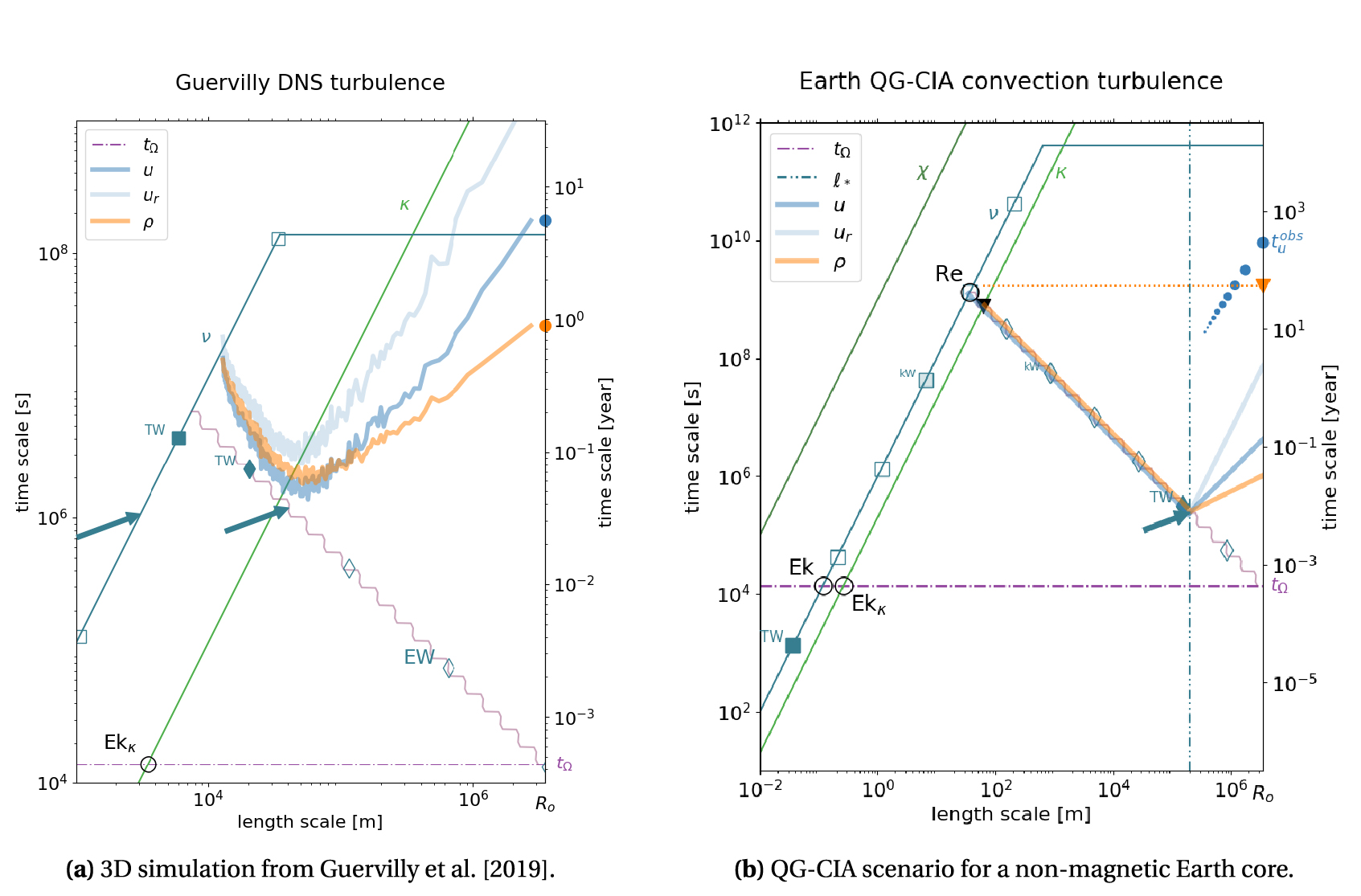
We first build its “template” as in Figure 2a, using radius Ro and t𝛺 (spin rate’s inverse) of the actual Earth’s core as length-scale and timescale, respectively, in order to compare with the Earth. Input dimensionless parameters Ek and Pr of the simulation provide values needed to build lines 𝜏𝜈(ℓ) = ℓ2∕𝜈 and 𝜏𝜅(ℓ) = ℓ2∕𝜅. As in Figure 2a, power dissipation markers are drawn along the Rossby and viscous lines, using outer core mass Mo. The simulation provides the power dissipated by viscosity in the bulk, pointed by a blue arrow on the viscous line, and the slightly larger viscous dissipation in the Ekman boundary layer, pointed by a blue arrow on the Rossby line.
We now turn to extracting lines 𝜏u(ℓ) and 𝜏𝜌(ℓ) from the simulation. Line 𝜏u(ℓ), labeled u, is obtained from the conversion of the volumetric average of a snapshot’s azimuthal order m-kinetic energy spectrum, following Equation (A57) of Appendix A.2.3. Note that line 𝜏u(ℓ) stays above the Rossby line at all length-scales, implying that the flow is quasi-geostrophic, as expected from the high degree of z-invariance observed in this simulation [Guervilly et al. 2019]. Remember that, in this case, length-scale ℓ has to be understood as the flow’s length-scale in the equatorial plane. Flow becomes anisotropic at large length-scale, as shown by the additional 𝜏u r(ℓ) line, labeled ur, of radial velocities. The azimuthal over radial velocity ratio increases with ℓ. Line 𝜏𝜌(ℓ), labeled 𝜌, is obtained in a similar way, using the conversion rule given by Equation (A59) of Appendix A.2.3, with gravity given by and Ra(Ro) = 2.5 × 10¹⁰.
Both 𝜏u(ℓ) and 𝜏𝜌(ℓ) lines display a sharp timescale minimum, very close to the Rossby line, defining length-scale ℓ⊥. This simulation thus nicely illustrates the QG-CIA force balance, with 𝜏Rossby(ℓ⊥) ∼𝜏u(ℓ⊥) ∼𝜏𝜌(ℓ⊥), as advocated by Guervilly et al. [2019]. Note that the same force balance appears to apply for ℓ < ℓ⊥, as envisioned by Rhines [1975]. Length-scale ℓ⊥ coincides with the length-scale given by power dissipation occurring in Ekman layers (blue arrow pinned to the Rossby line). As expected from Equations (13) and (5), viscous dissipation is mostly due to flow at the minimum 𝜏u(ℓ) time.
4.3. 𝜏–ℓ diagram for a non-magnetic Earth core
We now have all elements to start building a 𝜏–ℓ scenario for rotating convection in a non-magnetic Earth’s core, which we present in Figure 3b. The goal is to create and draw realistic 𝜏u(ℓ) and 𝜏𝜌(ℓ) lines over the background “template” of Figure 2a. We assume that viscous dissipation mainly occurs in Ekman layers. Applying Equation (13), we obtain time , which yields the dissipated power that we estimate for the Earth’s core (see Section 3.3), marked by a blue arrow in Figure 3b. We further formulate the ansatz of a QG-CIA force balance at the “optimum” length-scale ℓ∗, which thus lies on the Rossby line. We plot point (ℓ∗, 𝜏∗) in Figure 3b.
Inspired by Figure 3a, and by Rhines’ arguments, we infer that flow obeys the QG-CIA balance for all length-scales ℓ < ℓ∗. We thus plot 𝜏u(ℓ) and 𝜏𝜌(ℓ) lines along the Rossby line all the way to their intersection with dissipation 𝜏𝜈(ℓ) and 𝜏𝜅(ℓ) lines, respectively. It remains to draw lines 𝜏u(ℓ) and 𝜏𝜌(ℓ) for ℓ larger than ℓ⊥. Flow becomes anisotropic for ℓ > ℓ⊥, with radial velocities decreasing as ℓ increases, while azimuthal velocities increase with ℓ. For ℓ > ℓ⊥ we thus loosely prescribe 𝜏u r(ℓ) ∝ ℓ2 (for a spectral energy density E(k) ∝ k), 𝜏u a z(ℓ) ≃𝜏u(ℓ) ∝ ℓ (for E(k) ∝ k−1), and 𝜏𝜌(ℓ) ∝ ℓ1∕2 (for a k−2-spectrum).
Reading the 𝜏–ℓ diagram of Figure 3b, we see that core flow in a non-magnetic Earth would be quasi-geostrophic at all scales, with azimuthal velocities reaching 3 m⋅s−1, much larger than present-day core flow velocities represented by its value and trend. The radius of dominant columnar vortices would be around 200 km. Ekman layer viscous dissipation would dominate over bulk viscous dissipation by many orders of magnitude.
5. 𝜏–ℓ regime diagrams for the Earth’s core
In this section, we examine which 𝜏–ℓ regime diagrams to expect for the Earth’s core. Our goal is not to come up with an optimal or accurate scenario, but rather to illustrate how 𝜏–ℓ diagrams can help inventing and testing such scenarios. We now consider the presence of a magnetic field and try to document Earth’s core 𝜏–ℓ diagram, for which we presented a template in Figure 2b. Our starting point is the available convective power, as in Section 4.3. Building a turbulence scenario requires again estimating the balance of forces at different length-scales.
5.1. 𝜏–ℓ expression of force balances in rotating convective dynamos
Following the approach of Section 4.1, we add the Lorentz force in Navier–Stokes’ equation:
| (22) |
5.1.1. Magneto-Archimedean-Coriolis (MAC)
When magnetic Lorentz force is strong enough to break quasi-geostrophy at scale ℓ∗, one can get a balance between Lorentz, buoyancy and Coriolis forces, such that:
| (23) |
| (24) |
| (25) |
5.1.2. Quasi-geostrophic magneto-Archimedean-Coriolis (QG-MAC)
When the leading order force balance is quasi-geostrophic, the Coriolis term should only involve its ageostrophic part, at a length-scale ℓ∥∼ Ro. QG-MAC balance at lenght-scale ℓ⊥ therefore writes:
| (26) |
| (27) |
| (28) |
5.2. 𝜏–ℓ diagram of a remarkable numerical simulation
Let us start by building and discussing the 𝜏–ℓ regime diagram (Figure 4a) of one of the most extreme dynamo simulations available today: the S2 DNS of Schaeffer et al. [2017].
𝜏–ℓ diagrams for rapidly rotating convective dynamo. Refer to Figure 2b and Section 3 for a complete description of the background “template”. (a) 3D numerical simulation S2 of Schaeffer et al. [2017], Field variables u, b and 𝜌 of the simulation are represented by blue 𝜏u(ℓ), red 𝜏b(ℓ), and orange 𝜏𝜌(ℓ) lines, respectively, which are 𝜏–ℓ translations of their respective time- and volume-averaged degree n-spectra (see Appendix A.2.2). Simulation’s viscous dissipation can be read on line 𝜏𝜈(ℓ) at the blue arrow, while Ohmic dissipation is marked by a red arrow on line 𝜏𝜂(ℓ). The black vertical dotted line marks the length-scale at which a QG-MAC force balance appears to be achieved. (b) Scenario for the Earth assuming a MAC force balance. The available convective power TW sets time 𝜏∗ on the 𝜏𝜂(ℓ) line (red arrow). Length-scale of maximum dissipation ℓ∗≃ 7 km is obtained by combining Rm(ℓ∗) = 1 and a MAC force balance at this same length-scale. Circles labeled ℜ and Rm at the intersections of line 𝜏u with lines 𝜏𝜈(ℓ) and 𝜏𝜂(ℓ) mark the scales at which the corresponding ℓ-scale dimensionless number (see Table 2) equals 1. Red and blue stars on the right y-axis mark magnetic intensity and velocity amplitude, respectively, predicted by Christensen and Aubert [2006]’s scaling laws. Blue cross from Davidson [2013]’s velocity scaling law.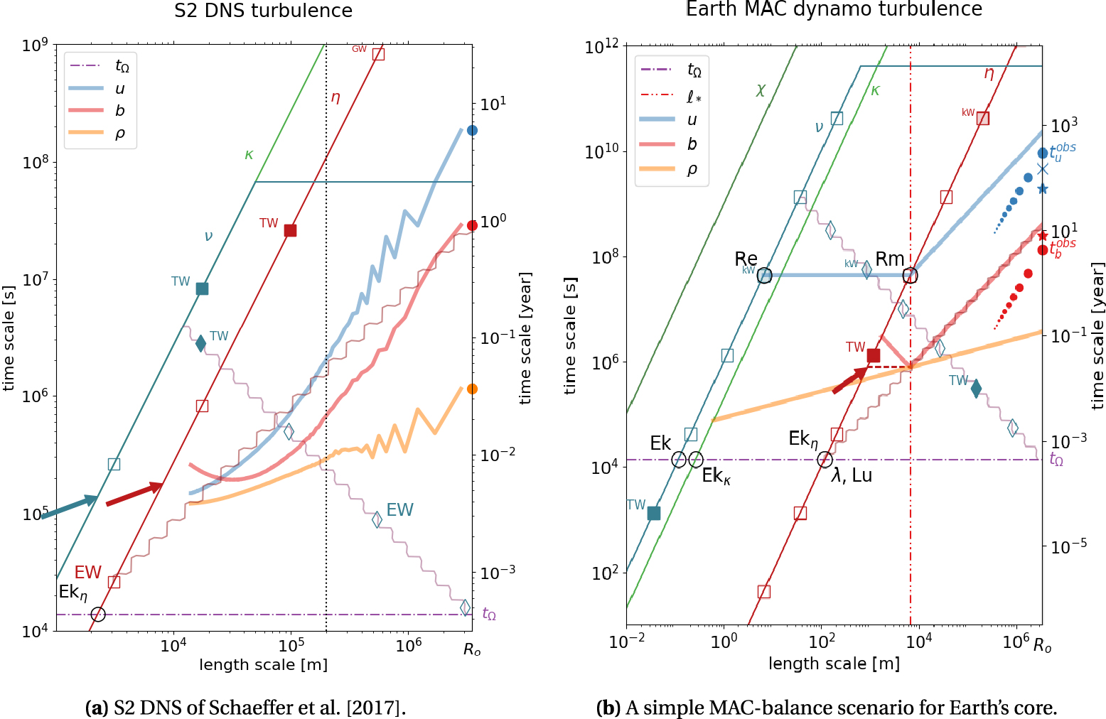
We first build its “template” as in Figure 2b, using radius Ro and t𝛺 of the actual Earth’s core as length-scale and timescale, respectively, in order to compare with the Earth. Input dimensionless parameters of the simulation (Ek(Ro − Ri) = 10−7, Pr = 1, Pm = 0.1) provide values needed to build lines 𝜏𝜈(ℓ), 𝜏𝜅(ℓ) and 𝜏𝜂(ℓ). As in Figure 2b, power dissipation markers are drawn and labeled along the magnetic diffusion line, and along the Rossby and viscous lines, using outer core mass Mo. Ohmic and viscous dissipations D𝜂 and D𝜈 of the simulation are obtained from Table 2 of Schaeffer et al. [2017], and scaled to Earth’s core by: . They are pointed by a red arrow on the magnetic diffusion line, and a blue arrow on the viscous line, respectively.
Next, we turn to extracting lines 𝜏u(ℓ) and 𝜏b(ℓ) from the simulation’s spherical harmonic spectra, applying conversion rules of Equations (A52) and (A53) of Appendix A.2.2, respectively. The simulated acceleration of gravity g at the top boundary is obtained from:
| (29) |
Reading the resulting 𝜏–ℓ diagram, we see that: magnetic energy largely dominates over kinetic energy (𝜏b(Ro)≪𝜏u(Ro)); Ohmic dissipation dominates over viscous dissipation (compare dissipation powers indicated by arrows pinned to lines 𝜏𝜂(ℓ) and 𝜏𝜈(ℓ), respectively); flow should be largely quasi-geostrophic, since the 𝜏u(ℓ) line stays above the Rossby line down to dissipation length-scales. We also observe that both 𝜏u(ℓ) and 𝜏b(ℓ) lines have slopes steeper than 1 at large length-scale, while the slope of the 𝜏𝜌(ℓ) line is closer to 1/2. Finally, we observe that a QG-MAC force balance seems approximately satisfied at length-scale ℓ⊥≃ Ro∕18, marked by a vertical dotted line, at which we observe (𝜏b∕t𝛺)(𝜏b∕𝜏u) ∼ Ro∕ℓ⊥ and 𝜏b(ℓ⊥) ∼𝜏𝜌(ℓ⊥).
5.3. A simple MAC-balance scenario
Figure 4b proposes a first attempt to complete the template of Figure 2b with plausible 𝜏u(ℓ), 𝜏b(ℓ) and 𝜏𝜌(ℓ) lines. As in Section 4.3, our starting point is the available convective power TW. We formulate the ansatz that it is dissipated by Joule heating only, which means that line 𝜏b(ℓ) should get down to (but not below) time that yields a dissipation equal to , as pointed by the red arrow on line 𝜏𝜂(ℓ). However, in contrast with the situation of Section 4.3, we cannot attach line 𝜏b(ℓ) to this point, because we anticipate that the velocity would be too weak at that scale to amplify the magnetic field.
One of the guidelines of our 𝜏–ℓ approach is that regime changes should occur where relevant ℓ-scale dimensionless numbers reach 1, i.e., at the intersection of corresponding 𝜏–ℓ lines. In a dynamo, we expect a regime change for Rm(ℓ) ∼ 1, at the intersection of lines 𝜏u(ℓ) and 𝜏𝜂(ℓ), below which magnetic diffusion takes precedence over induction. Furthermore, if the magnetic field is strong, the intensity of turbulence is strongly reduced in that low Rm regime. We thus assume that Ohmic dissipation is maximum at length-scale ℓ∗ where Rm(ℓ∗) = 1, implying 𝜏b(ℓ∗) ≃𝜏∗.
This first condition links the velocity field to the magnetic field but is not sufficient to provide ℓ∗. Another constraint is needed, which we get from a force balance. As a first guess, we request that our system obeys a MAC force balance at length-scale ℓ∗. Recalling Equation (24), we have:
| (30) |
The next step consists in drawing lines 𝜏u(ℓ) and 𝜏b(ℓ) for ℓ < ℓ∗ and for ℓ > ℓ∗. For ℓ < ℓ∗, we note that the regime of MHD turbulence in the presence of a strong magnetic field is characterized by steep energy density spectra: E(k) ∝ k−3 and Em(k) ∝ k−5 [Alemany et al. 1979]. Converting to 𝜏–ℓ language with Equation (A44), we get 𝜏u(ℓ) ∝ ℓ0 and 𝜏b(ℓ) ∝ ℓ−1, yielding the slopes drawn in Figure 4b. Adding rotation further reduces the intensity of turbulence [Nataf and Gagnière 2008, Kaplan et al. 2018], but we lack constraints on the resulting energy spectra.
In the dynamo region, for ℓ > ℓ∗, we assume k−1 energy density spectra for both u and b (i.e., 𝜏(ℓ) ∝ ℓ), implying that line 𝜏b(ℓ) follows the Alfvén wave line 𝜏Alfven(ℓ). This choice is mostly for pedagogical reasons as explained below. Finally, we rather arbitrarily assume 𝜏𝜌(ℓ) ∝ ℓ1∕2 at all length-scales. This completes the 𝜏–ℓ diagram shown in Figure 4b.
Reading this 𝜏–ℓ diagram, we see that our scenario yields velocity and magnetic amplitudes that are not too far from the observed and values. They translate into a magnetic to kinetic energy ratio of about 104, according to Equations (6) and (14). Bulk and boundary viscous dissipations have comparable amplitudes, both many orders of magnitude smaller than Ohmic dissipation, as assumed. The smallest QG vortices (on the Rossby line) are very sluggish, with a turnover time of about 1 year and a radius of 1 km. Magnetic diffusion is largest at a length-scale of about 10 km.
It is interesting to observe that our scenario implies that the Alfvén line intersects line 𝜏𝜂(ℓ) at time t𝛺, meaning that all three ℓ-scale dimensionless numbers Ek𝜂, Lu and 𝜆 equal 1 at this same scale. This implies that 𝜏b(Ro) can be deduced from the intersection of 𝜏𝜂(ℓ) and t𝛺 lines. In other words, even though our scenario has been built to achieve a given Ohmic dissipation , the actual value of 𝜏b(Ro) does not depend on . Only the kinetic energy depends on , as given by these scaling laws:
| (31) |
| (32) |
5.4. A simple QG-MAC balance scenario
The simple MAC-balance scenario of the previous section meets a problem: line 𝜏u(ℓ) plots above the Rossby line for all length-scales ℓ > ℓ∗, and all these scales have 𝛬d(ℓ) < 1. This means that flow should be quasi-geostrophic in this scale range, even though the magnetic field is strong. Leading-order force balance should therefore be quasi-geostrophic, with convective motions forming columnar vortices parallel to the spin axis. Figure 5a shows a first plausible alternative scenario, built as follows.
𝜏–ℓ diagrams of two QG-MAC force balance scenarios for the Earth core. Refer to Figure 2b and Section 3 for a complete description of the background “template”, and to Figure 4b for more details. Both scenarios assume that the available convective power TW is dissipated by Joule effect, setting time 𝜏∗ marked by a red arrow on the magnetic diffusion line, and that the flow obeys a QG-MAC balance at a prescribed length-scale ℓ⊥ = Ro∕10 indicated by a blue vertical dot-dash line. (a) a simple QG-MAC balance scenario. It is assumed that 𝜏u(ℓ) and 𝜏b(ℓ) are proportional to ℓ between ℓ∗ and Ro (see Section 5.4). (b) a QG-MAC balance scenario à la Aubert. This scenario assumes 𝜏u(ℓ) ∝ ℓ1∕2 for ℓ∗ < ℓ < ℓ⊥ (invariant vorticity) and 𝜏u(ℓ) ∝ ℓ3∕2 for ℓ⊥ < ℓ < Ro (following the trend of observations ). Same trends for 𝜏b(ℓ) (see Section 5.5).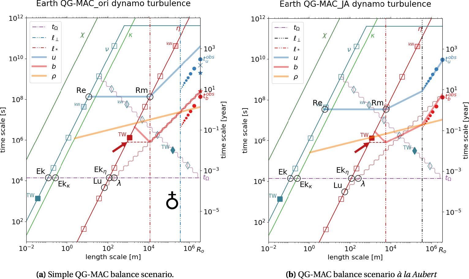
As in Section 5.3 we first obtain the minimum magnetic time 𝜏b, which is set to , marked by a red arrow on line 𝜏𝜂(ℓ), and the corresponding length-scale of maximum dissipation ℓ∗ is such that Rm(ℓ∗) = 1. This first condition links the velocity field to the magnetic field but is not sufficient to provide ℓ∗. Another constraint is needed, which we get from a QG-MAC force balance. We recall that such a balance at length-scale ℓ⊥ is given by Equation (27):
Graphically, this means that 𝜏b(ℓ⊥) plots at mid-distance between 𝜏u(ℓ⊥) and 𝜏Rossby(ℓ⊥). One then needs to guess at which scale ℓ⊥ this balance should apply. In contrast with our simple MAC scenario, one cannot choose ℓ⊥ = ℓ∗, because this would place 𝜏u(ℓ∗) very far down, below the t𝛺 line, breaking quasi-geostrophy, and yielding in strong disagreement with observations. And we also need to decide how velocity and magnetic fields vary between ℓ∗ and Ro. As in Section 5.3 we assume 𝜏u(ℓ) ∝ ℓ and 𝜏b(ℓ) ∝ ℓ. We then obtain:
| (33) |
Figure 5a displays the 𝜏–ℓ diagram of such a QG-MAC scenario with ℓ⊥ = Ro∕10. Comparing with Figure 4b, we see that this scenario predicts a larger magnetic over kinetic energy ratio, with 𝜏u above the Rossby line down to scales of a few hundred meters. Another difference is the level of line 𝜏𝜌(ℓ).
5.5. A QG-MAC balance scenario à la Aubert
In the previous scenario, choosing ℓ⊥ = Ro∕10 was borrowed from Aubert et al. [2017] and Aubert [2019], who find it in good agreement with their numerical simulation results. Following Davidson [2013], Aubert [2019] proposes a 𝜏u(ℓ) scaling for ℓ∗ < ℓ < ℓ⊥ that differs from the one we used in Section 5.4. In that interval, Davidson [2013] infers that vorticity is independent of ℓ. This translates into 𝜏u(ℓ) ∝ ℓ1∕2 instead of 𝜏u(ℓ) ∝ ℓ. Using the same scaling for 𝜏b(ℓ), length-scale ℓ∗ is then given by:
| (34) |
The corresponding 𝜏–ℓ regime diagram is shown in Figure 5b, where we chose to follow the observed ℓ3∕2 trend for 𝜏u and 𝜏b above ℓ⊥ (blue and red disks, respectively). This scenario provides an amazing fit to the observed and values. Furthermore, we observe that the dynamical Elsasser number 𝛬d(ℓ) = (t𝛺∕𝜏b(ℓ))(𝜏u(ℓ)∕𝜏b(ℓ)) remains below 1 at all length-scales ℓ, validating our assumption of leading-order Quasi-Geostrophy.
This scenario yields the following (ugly-looking) scaling laws for the largest scale velocity and magnetic fields:
| (35) |
| (36) |
5.6. The interesting case of Venus
The internal structure of Venus is very poorly known, but we know that it does not generate a detectable magnetic field. This important difference from its sister planet Earth is classically explained by a different thermal history, leading to a hot mantle convecting beneath a rigid lid, preventing core cooling, hence halting the convective engine of the dynamo [Stevenson et al. 1983, Nimmo 2002].
Venus and Earth also differ by their spinning rate: one turn in 243 days instead of one day. This difference is usually considered as unimportant since rotation still appears overwhelming, with an Ekman number Ek(Ro) ∼ 10−13 [Russell 1980]. However, if we adopt for Venus the same physical properties as for Earth, including its available convective power , but update the spinning rate to the one of Venus, we meet a problem, illustrated in Figure 6.
Devil’s advocate 𝜏–ℓ regime diagram for the core of Venus. All relevant properties are assumed identical to that of the Earth’s core (see Section 3.3), except for the spin rate (rotation period of 243 days). Venus “template” is built as in Figure 2b. Value s is deduced from an upper bound on Venus’ undetected magnetic field. We speculate that the difference in rotation period has a dramatic impact on the dynamo, and Section 5.6 proposes a tentative IMAC force balance scenario, which results in the displayed 𝜏–ℓ diagram.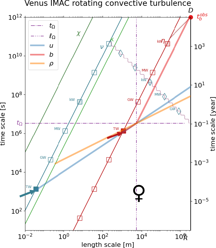
We first observe that Ohmic dissipation time plots below the t𝛺 line. We also see that the core of Venus would not be able to dissipate such a power by friction in its Ekman layers, as indicated by the markers along the Rossby line (compare with Figure 3b). Venus does not appear to be a “fast rotator”, and we should not expect the flow to be dominantly Quasi-Geostrophic as in Earth’s core. It might be more similar to the solar dynamo.
We therefore propose a very tentative “devil’s advocate” scenario, in which we assume that dissipation takes place in the bulk, with equipartioned viscous and Ohmic dissipations, yielding the blue arrow on the viscous line, and the red arrow on the magnetic diffusion line. In this region far below the t𝛺 line, Kolmogorov energy density spectra E(k) ∝ k−5∕3 seem plausible for both kinetic and magnetic energies, which translate into 𝜏u(ℓ) ∝ ℓ2∕3 and 𝜏b(ℓ) ∝ ℓ2∕3, as drawn in Figure 6 from their respective dissipation scales up to timescale t𝛺, which is met at a length-scale ℓ𝛺 ≃ 5 km.
The force balance we expect there is of type Inertia-Magneto-Archimedean-Coriolis (IMAC), given by:
| (37) |
Our exercise is very formal since we recall that there are good reasons to believe that such a convective power is not available for Venus [Stevenson et al. 1983, Nimmo 2002]. Nevertheless, our diversion to Venus questions the notion of “fast rotator” and shows that for a given convective power , planet’s spin rate might play a more important role than simply inferred from the low Ekman number it delivers.
6. Discussion
In this section, we try to show how 𝜏–ℓ diagrams can help building a new vision on several ongoing debates, such as the validity domain of various scaling laws and the controversy on the dominant length-scale in the core. We also illustrate the link with “path strategies” and propose extensions of this approach.
6.1. Validity domain of dynamo regimes
One goal of our approach is to better appreciate the validity domain of the various regimes encountered in planetary cores. For example, no dynamo will exist if line 𝜏u(ℓ) plots too high in the diagram, yielding Rm(Ro) ∼ 1. In Earth’s core, this would only happen for values several orders of magnitude smaller than our reference value of 3 TW. Actually, very low values (even negative) are not excluded by some thermal history models, before the birth of the inner core [e.g., Landeau et al. 2022].
At the other end, large values can pull the dynamo generation domain (Rm(ℓ) > 1) partly beneath the Rossby line. Complete columnar vortices won’t then have time to form at length-scales below the Rossby line, and we might have a somewhat different turbulence regime. Davidson [2014] proposed an original dynamo scenario that corresponds to such a situation. Noting that inertial waves are strongly helical, and that flow helicity is a key ingredient for dynamo action, he suggests that Earth’s dynamo might operate this way. None of the three scenarios we presented (Figures 4b, 5a, 5b) puts Rm(ℓ) ∼ 1 below the Rossby line. However, it would only take TW for the QG-MAC scenario à la Aubert (Figure 5b) to qualify (remember we only consider orders of magnitude).
An even more dramatic regime change should occur when 𝜏∗ < t𝛺, as in our devil’s advocate scenario for Venus (Figure 6). Then, the object should not be considered as a “fast rotator” anymore, and the dynamo regime is more of a small-scale type. This occurs when . For the Earth’s core, this translates into a power of 104 TW, which was never reached in Earth’s history.
We believe that 𝜏–ℓ diagrams could help inferring relevant dynamo regimes for planets and stars.
6.2. Dynamo scaling laws
Christensen [2010] nicely reviews a number of scaling laws proposed to infer the magnetic field intensity of planets (and stars). Among the nine proposed scaling laws he lists, five relate magnetic intensity to planetary rotation rate 𝛺, with no influence of the available convective power , three involve both 𝛺 and , and one only . The latter one, first proposed by Christensen and Aubert [2006], stems from the analysis of a large corpus of numerical simulations of the geodynamo, backed by an appraisal of the dominant terms in the governing equations. It is the law preferred by Christensen [2010] who shows that it is in good agreement with the measured magnetic intensity of planets and stars.
Translated in 𝜏–ℓ formulation, Christensen’s preferred laws yield:
| (38) |
| (39) |
Davidson [2013] re-examined this question and noted that inertia is playing too strong a role in Christensen and Aubert [2006]’s simulations. He derived a QG-MAC-balance variant and obtained a revised flow velocity law (his Equation (15)), which translates into:
| (40) |
Our discussion on scenario validity domain questions the obtention of universal dynamo scaling laws. However, we have seen that such scaling laws can be easily derived from the 𝜏–ℓ diagram of various scenarios. Each scenario produces 𝜏u(Ro) and 𝜏b(Ro) that combine 𝜏∗ (or Tdiss), T𝜂 and t𝛺 with various powers. Equations (31) and (32) give the scaling laws for a simple MAC scenario. Although built to dissipate a given convective power by Ohmic dissipation, this scenario provides a large-scale magnetic field B that does not depend upon , while U is independent of magnetic diffusivity 𝜂. The prediction of our QG-MAC scenario “à la Aubert” is given by Equations (35) and (36) for U and B, respectively.
6.3. Dominant length-scale controversy
Several recent studies have revived a debate on the dominant length-scales to be expected in the Earth’s core [Yan et al. 2021, Bouillaut et al. 2021, Yan and Calkins 2022, Cattaneo and Hughes 2022, Nicoski et al. 2024, Abbate and Aurnou 2023, Hawkins et al. 2023]. Fast rotation inhibits thermal convection, and viscosity is needed to break the Taylor–Proudman constraint [Chandrasekhar 1961]. Studies on the onset of thermal convection in rapidly rotating plane layers [Chandrasekhar 1961], annulus [Busse 1970], and spherical shells or spheres [Busse 1970, Jones et al. 2000, Dormy et al. 2004] therefore all show that, at the onset of convection, the flow consists in columnar vortices aligned with the rotation axis, with a width ℓc ∼ Ro[Ek(Ro)]1∕3 (see Appendix B). In the Earth’s core, such columns would be 30 m in diameter, extending several thousand kilometers in length. At least two effects could strongly widen such columns: (i) the magnetic field [Chandrasekhar 1961, Fearn 1979, Sreenivasan and Jones 2011, Aujogue et al. 2015]; (ii) non-linear flow advection [Rhines 1975, Ingersoll and Pollard 1982, Gillet et al. 2007, Jones 2015, Guervilly et al. 2019].
The effect of the magnetic field can be studied at the onset of convection, but only for given—often simplistic—geometries of the magnetic field that never occur in natural systems. These studies show that convective cells can get as large as the depth of the container Ro when a magnetic field is present. Concerning planetary dynamos, one can argue that such an effect can only be invoked when the dynamo has already produced a strong enough magnetic field. This led Cattaneo and Hughes [2022] to call on the Moon for help, arguing that in an unmagnetized Earth, “convection would consist of hundreds of thousands of extremely thin columns” that would be unable to produce a magnetic field.
This view is clearly challenged by Guervilly et al. [2019] who advocate a dominant convective length-scale around 30 km. Their prediction rests on the extrapolation of a QG-CIA force balance to Earth’s core conditions, and is backed by numerical simulations such as the one we present in Figure 3a. Our QG-CIA scenario, shown in Figure 3b obeys the same rules. It predicts an even larger dominant length-scale (∼200 km) because it is built on the available convective power rather than on the observed large-scale velocity, which is reduced by the magnetic field. Interestingly, Figure 3a shows that the simulations of Guervilly et al. [2019] remain very close to the convection onset, which would yield a critical length-scale ℓc close to the intersection of the 𝜏𝜅(ℓ) and 𝜏Rossby(ℓ) lines (see Appendix B). Yet, they reach a turbulent QG-CIA balance because of the low value of the Prandtl number (Pr = 10−2) that allows for large Reynolds numbers near the onset [Aubert et al. 2001, Kaplan et al. 2017].
Our 𝜏–ℓ diagrams clearly emphasize the role of in controlling the dominant length-scale, both with and without a magnetic field. This is particularly clear in Figure 3b where the minima of curves 𝜏u(ℓ) and 𝜏𝜌(ℓ) would “slide” along the Rossby line following the blue arrow. This diagram also suggests that while viscosity in the bulk controls the convective length-scale at the onset (black triangle), it progressively looses its importance as viscous dissipation in the Ekman layers takes over. To achieve a turbulent convection regime where viscosity in the bulk is unimportant, it is crucial to provide another way of dissipating the convective power, like Ekman layer friction or Ohmic dissipation, which are both present in Earth’s core. Because you always need to dissipate the power injected into turbulence, the previous sentence sounds rather obvious. Yet, this might explain why several recent studies find no evidence of a diffusion-free scaling, in which viscosity plays no role. In the numerical simulations of Yan et al. [2021], Yan and Calkins [2022], Nicoski et al. [2024], boundaries are stress-free so that no other energy sink than viscous dissipation in the bulk can equilibrate the convective power.
6.4. Path strategy
Our 𝜏–ℓ approach has much in common with the “path strategy” devised by Julien Aubert and colleagues [Aubert et al. 2017, Aubert and Gillet 2021, Aubert et al. 2022, Aubert 2023]. Their strategy also targets the dynamical regime of a given object, the Earth’s core, and aims at defining a “path” that numerical simulations should follow to reach that regime. As stressed by Dormy [2016], minimizing Pm at a given Ekman number is not a good strategy, since it increases magnetic Ekman number , while Christensen et al. [2010] show that Ek𝜂(Ro) < 10−4 is needed for obtaining Earth-like geodynamo simulations. Hence the need for targeting a more elaborate “distinguished limit” [Dormy 2016].
Aubert and his colleagues stress the importance of respecting the hierarchy of dynamic times, and propose a unidimensional path based on scaling laws obtained by Davidson [2013] for a QG-MAC force balance. Position along the path is measured by an 𝜖 parameter. As exposed in Aubert [2023], the idea is to keep the magnetic diffusion time T𝜂 =𝜏 𝜂(Ro) fixed to the Earth value, and to decrease the magnetic Ekman number step by step, by decreasing the rotation time t𝛺 from values at which appropriate numerical simulations are available (defining 𝜖 = 1) down to the actual value of the Earth (𝜖 = 10−7). Long-period behaviour of the Earth’s core is well recovered from 𝜖 = 1, while decreasing 𝜖 to Earth’s value allows for the development of short-term dynamics.
Figure 7 shows how 𝜏–ℓ diagrams can help visualize and extend this strategy. We show three diagrams, which correspond to three different values of 𝜖: 1, 10−3, and 10−7. Their “template” are built from the values of the magnetic Ekman and Prandtl numbers listed for “prior PB” in Table 1 of Aubert [2023]. The values of (red arrow), (blue disk), and (red disk), are from the corresponding simulation outputs given in his Table 2. We then add the 𝜏𝜌(ℓ), 𝜏u(ℓ) and 𝜏b(ℓ) lines that our “à la Aubert” QG-MAC balance scenario (see Section 5.5) predicts for the listed . An amazing fit of the “observed” tu and tb is obtained, choosing ℓ⊥ = Ro∕5.
𝜏–ℓ regime diagrams illustrating the “path strategy” devised by Aubert and colleagues. (a) 0% of path (𝜖 = 1). (b) 43% of path (𝜖 = 10−3). (c) 100% of path (𝜖 = 10−7). See text for explanations.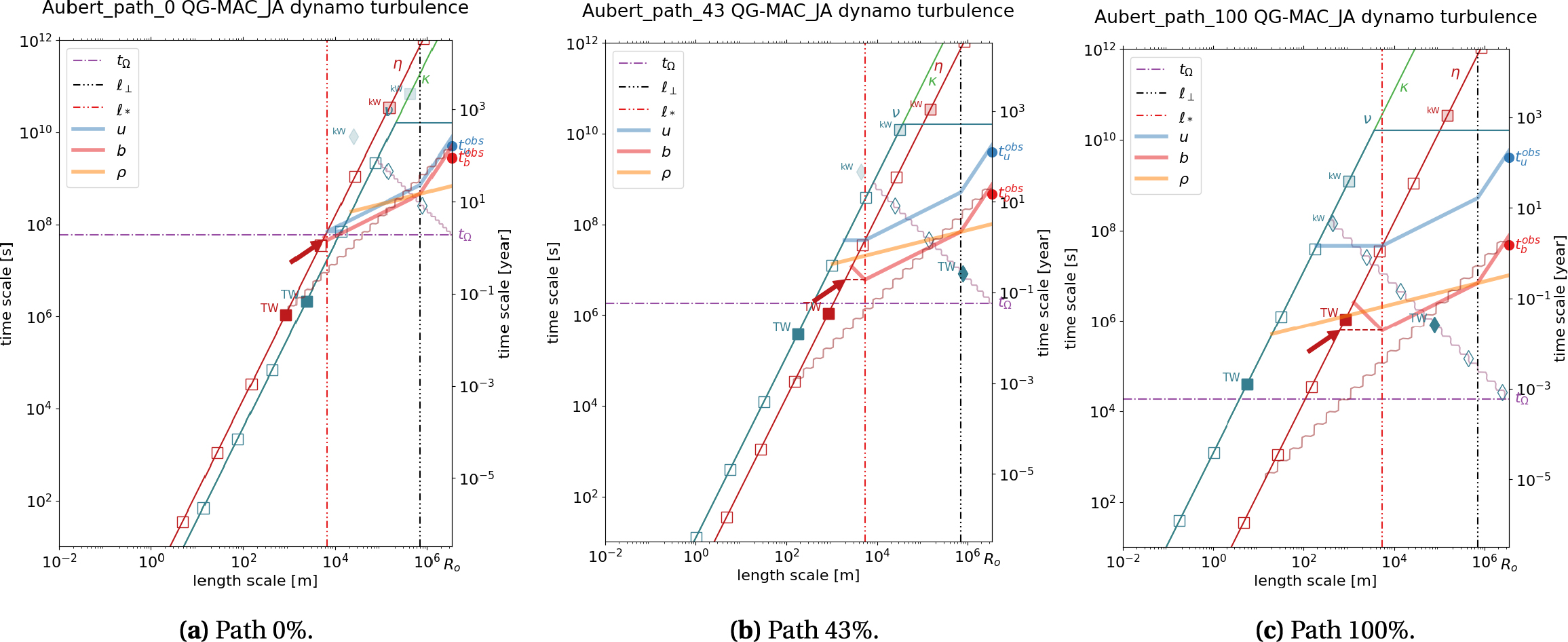
A key contribution of Aubert and colleagues was to determine how the input parameters of numerical simulations should scale with 𝜖 in order to follow the path. This is where the QG-MAC scaling laws of Davidson [2013] come in, and this is also where 𝜏–ℓ diagrams can help. Using the scaling laws obtained for 𝜏u(Ro) and 𝜏b(Ro) in Section 5.5, we test two different paths. Note that parameter 𝜖 is defined such that , implying .
Aubert and colleagues chose to keep Rm(Ro) constant along the path, i.e., 𝜏u(Ro)[𝜖] = Ct e. Equation (35) then implies , since T𝜂 does not vary with 𝜖, and assuming that ℓ⊥∕Ro is constant as well. We thus get since . Equation (36) then implies 𝜏b(Ro)[𝜖] ∝𝜖1∕2. These scalings agree with those of Aubert [2023], as can be seen in Figure 7.
Instead of keeping Rm(Ro) constant along the path, one could choose to keep the dynamo-generating domain above the Rossby line, as we obtain for the Earth. Imposing that Rm(ℓ) = 1 occurs at the intersection of lines 𝜏𝜂(ℓ) and 𝜏Rossby(ℓ) yields 𝜏u(Ro)[𝜖] ∝𝜖1∕4, 𝜏b(Ro)[𝜖] ∝𝜖3∕8, and . It would be interesting to run numerical simulations along such a path.
7. Limitations and perspectives
Let us first recall that our 𝜏–ℓ approach is not a theory of turbulence. We try to formulate plausible scenarios by identifying scales at which a change in turbulence regime should occur, and by patching scaling laws appropriate for each regime. We thus entirely depend on the availability of such laws, which can be brought by experiments, theory, and numerical simulations.
Our approach contains a fair number of assumptions and approximations. How realistic are the conversion rules we employ to “translate” force balances and turbulent spectra in 𝜏–ℓ language? Does the minimum dynamic time control dissipation? What controls length-scale ℓ⊥ that we had to guess for writing QG-MAC-type force balances?
For simplicity reasons, we have treated planetary cores as simple full spheres. The application to actual planets requires to at least consider spherical shells of various thicknesses instead. An extension to giant planets and stars also requires taking into account compressibility and free-slip boundaries.
Our results suggest that dissipation of Quasi-Geostrophic flows in Ekman layers takes over bulk dissipation in rapidly rotating convection when it gets strongly super-critical. Can it be tested? How smooth is the transition? Our devil’s advocate scenario for Venus suggests a transition to a very different regime if dissipation is too large to be taken up by Ekman friction. Is there evidence for such a transition? How sharp is it?
We observe that density anomaly spectra from numerical simulations are rarely displayed, while they convey valuable information. We also note that spectra from laboratory experiments are scarce (but see Madonia et al. [2023]) and too often given in “arbitrary units”, preventing their conversion into 𝜏–ℓ representation. We are lacking experimental data on turbulence for rotating convection in a sphere in presence of strong magnetic fields.
𝜏–ℓ diagrams provide hints on how velocity and magnetic field scale with length-scale. This might be useful for observers who need such constraints to tune their magnetic field and core-flow inversions [Gillet et al. 2015, Baerenzung et al. 2016]. As a matter of fact, our analysis suggests that the flat spherical harmonic spectra observed at low degrees n for both flow velocity and magnetic field cannot extend much beyond degree 10 without meeting dissipation problems.
8. Conclusion
𝜏–ℓ regime diagrams are a simple graphical tool that proves useful for inventing or testing dynamic scenarios for planetary cores. Tradition in fluid dynamics is to characterize systems by dimensionless numbers, usually based on “typical” large-scale quantities. Past decades have seen large efforts to develop a more detailed description of phenomena that operate at different scales. This has led to the apparition of even more dimensionless numbers, in which the various scales involved do not always figure very clearly, and to the construction of somewhat unintelligible scaling laws. By defining 𝜏 timescales that depend on ℓ length-scales over their entire range, we hope to make these choices more explicit. By providing a simple graphical identity to these scales, we wish to make their meaning more intuitive. Contrary to spectra in “arbitrary units”, 𝜏–ℓ diagrams give insight into regimes and balances which are paramount to rotating, magnetized and/or stratified fluids, where waves can be present and significantly alter the dynamics.
Because they put together most key properties of a given object, 𝜏–ℓ regime diagrams constitute a nice identity card. We think this applies to numerical simulations and laboratory experiments as well. Both approaches enable extensive parameter surveys, which are crucial for exploring and understanding different regimes. Being object-oriented, 𝜏–ℓ diagrams are not easily applied to such surveys, but we think they would very valuably complement classical scaling law plots. The idea would be to draw 𝜏–ℓ diagrams for a few representative members and end-members of the survey, which would nicely illustrate their validity range.
Our article thus has two goals. The first goal is to provide all ingredients for building your own 𝜏–ℓ diagram, be it of a numerical simulation, a laboratory experiment or theory. To that end, we included construction rules, examples, technical appendices, and Python scripts (supplementary material). The second goal is to demonstrate the potential of 𝜏–ℓ regime diagrams for suggesting and testing various scenarios for Earth’s dynamo.
Convinced that available convective power is a key control parameter, and the one that can most readily be estimated for other planets and exoplanets, we have modified our original approach [Nataf and Schaeffer 2015] to propose and discuss a few scenarios built upon this input data. This results in a more challenging exercise, calling for force balance inspection. We show that the 𝜏–ℓ translation of relevant force balances is very handy and telling.
We built several geodynamo scenarios to test MAC (Figure 4b) and QG-MAC (Figure 5a, 5b) force balances. The validity domain of these scenarios shows up well in 𝜏–ℓ diagrams. A QG-MAC scenario “à la Aubert” looks particularly appealing, and could have applied to the Earth over its entire history. We note that in such a scenario, flow in the dynamo-generating region remains Quasi-Geostrophic, with a dynamical Elsasser smaller than 1, even though the magnetic to kinetic energy ratio is of order 104. In contrast, Venus would have a hard time entering that regime, because of its slow rotation (Figure 6). This calls for a re-analysis of what is called a “fast rotator”.
𝜏–ℓ regime diagrams also help us addressing several on-going debates, such as the the validity of various scaling laws, and the question of the dominant convective length-scale in the Earth’s core. We speculate that dissipation in Ekman layers drives non-magnetic rapidly rotating convection towards a QG-CIA force balance when the flow is turbulent enough, promoting dominant length-scales much larger than the iconic Ro Ek1∕3 length-scale at convection onset (Figure 3b).
We use 𝜏–ℓ diagrams to illustrate the concept of “path strategy” developed by Julien Aubert and colleagues (Figure 7), and we propose an interesting alternative to their original path.
Declaration of interests
The authors do not work for, advise, own shares in, or receive funds from any organization that could benefit from this article, and have declared no affiliations other than their research organizations.
Dedication
The manuscript was mostly written by HCN. NS ran all presented numerical simulations. Both authors have given approval to the final version of the manuscript.
Acknowledgments
We thank the French Academy of Science and Electricité de France for granting their “Ampère Prize” to our “Geodynamo” team, and Bérengère Dubrulle for early encouragements. HCN thanks Peter Davidson, Julien Aubert, Thomas Gastine, Franck Plunian, Sacha Brun, Antoine Strugarek and Quentin Noraz for useful discussions, and Emmanuel Dormy for his review. The authors would like to thank the Isaac Newton Institute for Mathematical Sciences, Cambridge, for support and hospitality during the programme “Frontiers in dynamo theory: from the Earth to the stars” where work on this paper was undertaken. This work was supported by EPSRC grant no EP/R014604/1. ISTerre is part of Labex OSUG@2020 (ANR10 LABX56). Our manuscript greatly benefited from the thorough reviews of three anonymous referees (including rather harsh but stimulating comments by a “lengths and time scales person”).
A.1. Choosing a conversion rule
We consider different expressions of total energy per unit mass :
| (A41) |
A flow with spectral energy density E(k) ∝ k−5∕3 yields the same k-exponent for its discrete energy spectrum EB [Lesieur 2008, Stepanov et al. 2014], and a n−5∕3 Lowes–Mauersberger spectrum. However, pre-factors may differ. More importantly, the conversion of energy spectra into 𝜏–ℓ equivalents is questionable. Indeed, no exact conversion between spectral energy density and eddy velocity can be drawn, as thoroughly discussed by Davidson and Pearson [2005].
In Kolmogorov [1941]’s universal turbulence, an eddy turnover time is classically derived as:
| (A42) |
In our object-oriented approach, the integral length scale Ro plays a role, and when translating numerical simulation energy spectra in 𝜏–ℓ form, we were thus tempted to simply define 𝜏u(ℓ) as where is the degree n component of the spherical harmonic spectrum of u2, and ℓ(n) is given by:
| (A43) |
We thus use conversion rules similar to that of Equation (A42), such as:
| (A44) |
A.2. Application to various relevant spectra
We now detail the 𝜏–ℓ conversion of spectra commonly obtained from observations, numerical experiments and laboratory experiments.
A.2.1. Lowes–Mauersberger spectrum
In geomagnetism, the variation of magnetic energy with length-scale is usually measured by its Lowes–Mauersberger spectrum [Lowes 1966]. This spectrum is expressed in terms of Gauss coefficients and of scalar magnetic potential V , which defines the internal magnetic field at any radius above the core-mantle boundary when the mantle is considered as an electrical insulator.
Potential V (r,𝜃,𝜑) is then solution of Laplace equation and can be expressed in terms of spherical harmonics as:
| (A45) |
Following Langlais et al. [2014], the Lowes–Mauersberger spectrum at any r > Ro is then given by the suite of defined by:
| (A46) |
| (A47) |
| (A48) |
| (A49) |
| (A50) |
A.2.2. Degree n-spectra from numerical simulations
Numerical simulations of planetary dynamos are most often performed using a pseudo-spectral expansion in spherical harmonics of degree n and order m. Degree-n or order-m spectra are thus readily obtained for both velocity, magnetic and codensity fields. These spectra are usually for u2, b2 and C2 in dimensionless units, such that the sum over all n and m yields 2∕𝜌 times the energy per unit mass of that dimensionless field. Given length-scale L and time-scale T chosen in the simulation, u and b spectra should be multiplied by L2∕T2 (assuming that b is expressed in Alfvén wave velocity units).
Given these precisions, the procedure is similar to that exposed in Appendix A.2.1. ℓ(n) is still given by:
| (A51) |
| (A52) |
| (A53) |
| (A54) |
In the example of Figure 3a from Guervilly et al. [2019], the simulated acceleration of gravity g at the top boundary is obtained from:
| (A55) |
In the example of Figure 4a from Schaeffer et al. [2017], g is obtained from:
| (A56) |
A.2.3. Order m-spectra from numerical simulations
Quasi-geostrophic vortices are better characterized by their order-m spectra than by their degree-n spectra, in particular in 2D QG simulations. Thus Guervilly et al. [2019] display m-spectra of their 3D and QG convection simulation results. Translation into 𝜏–ℓ is obtained as in Appendix A.2.2, replacing by :
| (A57) |
| (A58) |
| (A59) |
| (A60) |
For the simulation presented in Figure 3a, and spectra are very similar, apart for even-odd oscillations in the n-spectra due to equatorial symmetry.
A.2.4. Frequency spectrum
In laboratory experiments, turbulent spectra are more easily obtained from signal x(r,t) measured in the time-domain (t = 0 to T) at a given position r. Power spectral density (PSD) is then computed from its Fourier transform as:
| (A61) |
When a mean flow U(r) is present, and when turbulence is weak enough, a time record of velocity reflects the advection of the spatial variation of velocity [e.g., Frisch 1995]. Extensions to intense turbulence have been developed [Pinton and Labbé 1994]. Taylor’s hypothesis [Taylor 1938] then permits to obtain a kinetic energy density wavenumber spectrum E(r,k) from the velocity frequency power spectrum :
| (A62) |
Note that Taylor’s hypothesis cannot be applied to magnetic spectra unless magnetic diffusion is small enough for the frozen flux approximation to apply.
1 Note that one can define a dissipation time , which makes it more explicit that is independent of magnetic diffusivity 𝜂.