


 CC-BY 4.0
1. Introduction
Seismic wave attenuation illustrates the energy losses during wave propagation and is often quantified through the inverse of the quality factor, Q. The energy losses are mainly the result of scattering and fluid-related mechanisms. Scattering describes the losses due to multiple small reflections caused by the heterogeneities of the subsurface [Wu and Aki 1988], while fluid-related mechanisms such as wave-induce fluid flow (WIFF) describes the energy losses due to the frictional movement between solid grains and pore fluids [e.g., Murphy et al. 1986; Müller et al. 2010]. Thereby, seismic attenuation might be an efficient seismic attribute for studying heterogeneous and fractured media such as carbonate reservoirs. Indeed, several attenuation studies have been successfully conducted with applications in the petroleum industry [e.g., Bouchaala and Guennou 2012; Matsushima et al. 2018], seismology [e.g., Del Pezzo et al. 2019; Prudencio et al. 2013], and civil engineering [e.g., Boadu 1997; Li et al. 2018]. Mavko and Nur [1979], who developed one of the earliest models describing seismic wave attenuation in saturated rocks, reported a strong increase in attenuation induced by a small amount of free gas. Several subsequent studies investigated attenuation in partially saturated media [e.g., Bouchaala and Guennou 2012; Müller et al. 2010], and most of them confirmed the strong magnitude of attenuation as observed by Mavko and Nur [1979]. Moreover, the direct link between fluid viscosity and attenuation allowed Shabelansky et al. [2015] to use the latter as a proxy to monitor the viscosity changes during the heating of heavy oil reservoirs, and hence to manage the production.
The combination of compressional and shear attenuations can help to enhance reservoir characterization by allowing more reservoir properties to be obtained than by the use of a unique attenuation mode. Winkler and Nur [1982] observed that the magnitude of the attenuation ratio QS∕QP is higher than 1 in partially saturated rocks and less than 1 in fully saturated rocks. They also noticed that the attenuation ratio is more sensitive to the presence of the gas than the velocity ratio. Klimentos [1995] noticed QS∕QP > 1 in rocks containing gas or condensate, and the opposite in rocks fully saturated with water or with water and oil. Hence, the attenuation ratio QS∕QP may help to distinguish between gas and condensate from oil and water. Qi et al. [2017] also estimated and from sonic waveforms and suggested that the magnitude of QS∕QP is largely controlled by gas saturation.
Even though the use of S wave attenuation may be largely useful for reservoir characterization, the difficulty of its extraction from field data makes the most in situ attenuation studies to be based on only P waves. The high heterogeneous nature of carbonate rocks increases the difficulties of the extraction of shear waves. The few seismic in situ attenuation studies carried out in carbonates rocks were mainly based on P waves [e.g., Bouchaala et al. 2016b, 2014]. The S wave attenuation in carbonate rocks is usually estimated either from sonic waveforms [e.g., Bouchaala et al. 2019a; Matsushima et al. 2018] or in laboratory at ultrasonic frequencies [e.g., Adam et al. 2009; Assefa et al. 1999], because in both cases S waves are generated and recorded separately from P waves. Bouchaala et al. [2016a] studied the attenuation of a carbonate reservoir in Abu Dhabi. They noticed a high dispersion of the values of the fast and slow sonic shear waves ratio (QS2∕QS1) with depth in highly fractured zones, and small dispersion in slightly fractured zones. Adam et al. [2009] calculated and from five carbonate samples with different petrophysical properties. Curiously and in contrast to most of sandstone observations, they found that QS∕QP > 1 in dry and fully saturated media, and QS∕QP < 1 in partially saturated media. They also reported a compressional attenuation increase of 250% after the substitution of brine by light hydrocarbon in the samples. Therefore, including shear waves in the in situ attenuation studies of Abu Dhabi carbonate reservoirs may help in providing clear-sightedness on the magnitude of QS∕QP and its dependence on petrophysical properties of the reservoir zones.
The aim of this study is to estimate attenuation from downgoing P and S waves that are properly extracted from three-component (3C) vertical seismic profiling (VSP) data acquired over an offshore Abu Dhabi oilfield. For a proper extraction of P and S waves, the 3C raw VSP data were carefully processed by trying to preserve the amplitudes as much as possible, then rotated in order to maximize the shear energy. After that, wavefields were separated to produce four independent wavefields: downgoing P, downgoing S, upgoing P, and upgoing S. We applied the spectral ratio method [Bath 1974; McDonal et al. 1958] to estimate QP and QS from the downgoing waveforms. Furthermore, we estimated compressional and shear sonic attenuations, which permits the investigation of frequency dependence of attenuation.
(a) The acquisition geometry of 3D VSP data acquired with seventy receivers placed 20 m apart [modified from Bouchaala et al. 2019b]. (b) Map view of shot locations.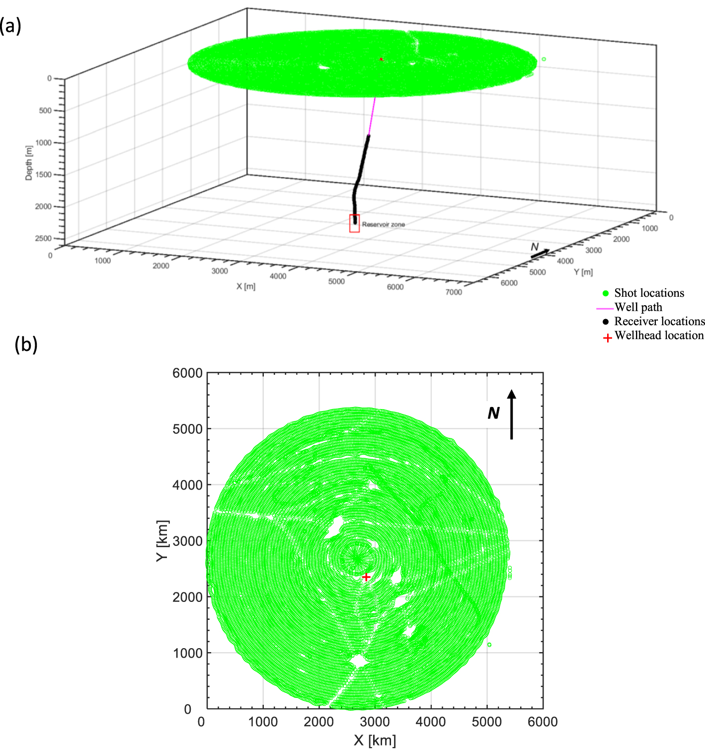
2. Study area and field data
The oilfield is an east–west plunging anticline, located in offshore Abu Dhabi, United Arab Emirates (UAE). The oilfield is characterized by gentle dips with steepest dips occurring in the north and northeast where the average dip is about 2.5°. The stratigraphy of the oilfield is mostly made of carbonates of Mesozoic–Cenozoic in age. The reservoir zones are made of stacked sections of porous, shallow water carbonates of the Lower Cretaceous Thamama Group. The studied reservoirs are divided into three zones: TH1, TH2, and TH3. The average reservoir porosity ranges from 10 to 25% and the permeability from 10 to 100 md. Fractures have been reported in TH1 and TH3 [Edwards et al. 2006; Skeith et al. 2015]. These fractures generally occur at the boundaries of dense zones and reservoir units [Shekhar et al. 2017].
The 3C 3D VSP data were acquired with a maximum source offset of 3000 m from the wellhead. Seventy receivers were placed 20 m apart in the wellbore to record the data generated by 18047 shots with average shot spacing of 25 m (Figure 1). Due to weather conditions and obstacles such as platforms, the survey geometry was not shot regularly as originally planned, though its coverage is very good. The extracted shots at near (200 m), middle (1050 m), and far (2500 m) offsets (Figure 2) show that the overall data quality is good except at far offset, in the depth range of 1145–1525 m (receivers 1–20) and at the depth of 1705 m (receiver 29). Furthermore, receiver 60 at the depth of 2325 m did not record any data (Figure 2).
Vertical Z (a, b, c), horizontal X (d, e, f) and Y (g, h, i) components of raw VSP data recorded at near offset (a, d, g), middle offset (b, e, h) and far offset (c, f, i).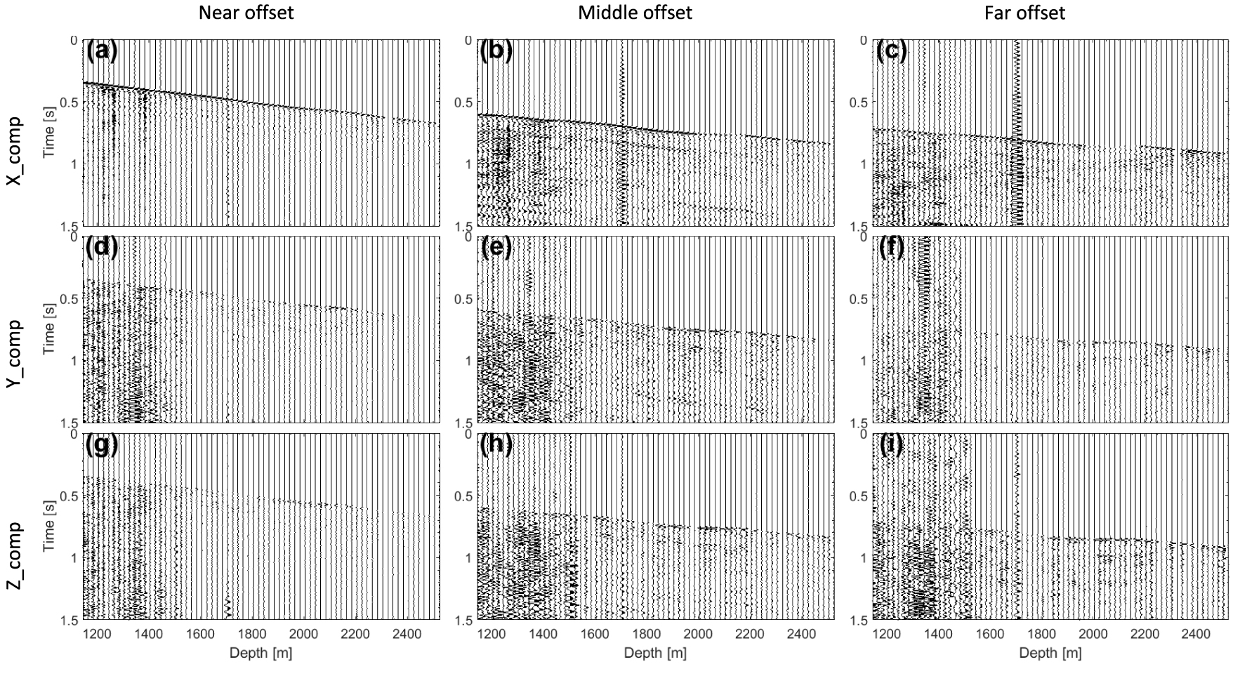
The relative bearing (RB) technique [e.g., Armstrong 2005; Kazemi and Naville 2017] was applied to rotate the data from the local reference frame to the geographic coordinate system (north–south, east–west, and true vertical). The RB angles were recorded by the RB sensor, which is a weighted potentiometer, located between the X and Y receivers. As the tool tilts in a deviated well, the RB sensor measures the position of the X axis relative to the well azimuth. The RB angles were used along with the azimuths of the well deviation to orient the receivers in the geographic coordinate system. Furthermore, the anomalous amplitude attenuation (AAA) processing was applied in order to reduce the random noise and abnormal spikes in the data. The AAA technique transforms the data into the frequency domain and applies a spatial median filter [e.g., Guo and Lin 2003; Wu et al. 2017]. Then, the Wavesip method [Leaney 2002] was used to decompose the 3C component data into P, Sv upgoing, and downgoing wavefields (Figure 3). In this method, the slowness and the polarization of each plane wave are calculated. Then, a linear system is solved in the frequency domain in order to compute plane-wave amplitudes. Finally, a summation by wave types (downgoing P, downgoing Sv, upgoing P, and upgoing Sv) is performed over the plane waves to separate the wavefields. The noisy data and dead traces were not used in the wavefield separation. The Wavesip method can handle anisotropic media and it can preserve the amplitudes, which permits the use of the decomposed wavefields for AVO analysis, prestack migration, and attenuation analysis [Graves et al. 2008; Leaney 2002]. Furthermore, this method is well appropriate for 3D VSP data acquired with large receiver array [Leaney 2002]. More details about the Wavesip method are provided in Appendix A.
Sonic data were also acquired in the reservoir zones during the VSP experiment by using a high-resolution (0.1524 m) dipole sonic imager (DSI) (Figure 15). The DSI tool allows a separate acquisition of compressional monopole (mo) and shear dipole (xd) waveforms. However, due to a limitation in data quality, we only used the sonic waveforms recorded in the depth range of 2294–2389 m (Figure 4), which covers the reservoir zone TH1 and the uppermost part of the reservoir zone TH2. The high resolution of sonic waveforms allows a direct comparison between the attenuation and the other petrophysical logs recorded with the same resolution.
Separated compressional (a, b, c) and shear (d, e, f) wavefields at near offset (a, d), middle offset (b, e) and far offset (c, f).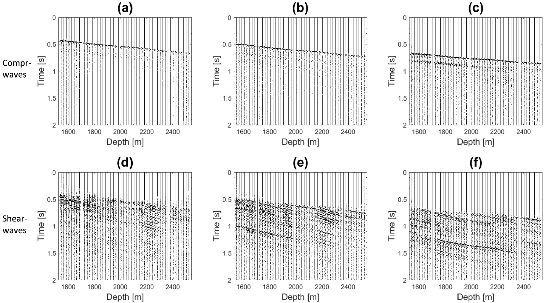
Monopole (mo) and dipole (xd) waveforms recorded at one of the DSI receivers in the reservoir zones.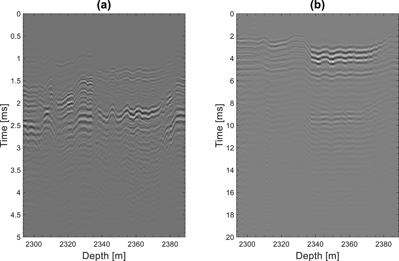
(a) Map view of the selected shots for the attenuation study. The shots are lined up along the north–south direction with an accuracy of ±5°. The red triangle indicates the VSP wellhead. (b, c, d) Receiver gathers of downgoing S waves at depths of 1925 m, 2185 m, and 2305 m, respectively. The dashed red curves indicate waveforms generated from P waves converted at the top of Fiqa Formation from which shear wave attenuation was estimated.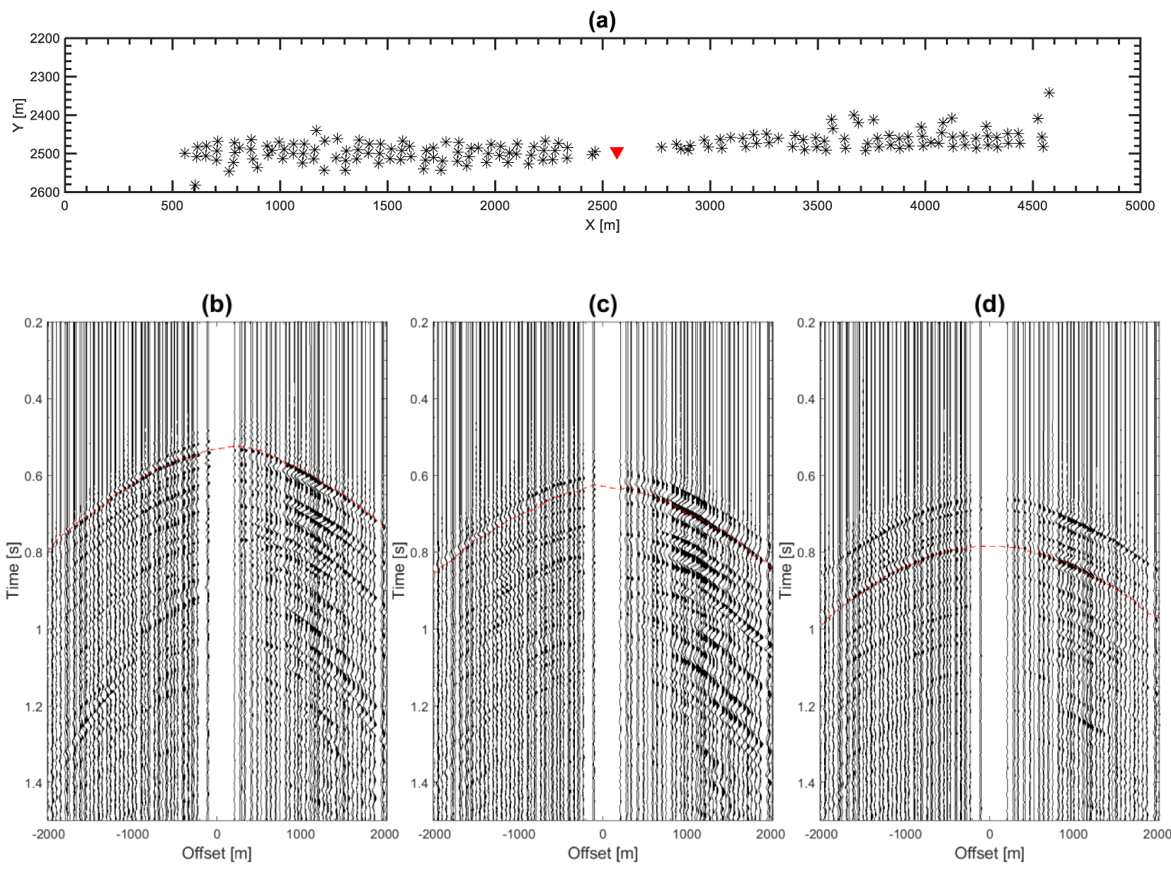
3. Estimation of VSP attenuation
We generated receiver gathers from downgoing P and S wavefields of shots that have azimuths close to the north–south direction with an accuracy of ±5° (Figure 5a). After a meticulous analysis of the receiver gathers of downgoing waves, we noticed that the seismic event indicated by red curves in Figures 5b–d, has a good signal to noise ratio (SNR) in most of receivers with the highest SNR at the offset range of 817–1218 m. Therefore, we selected this seismic event at these offsets for the estimation of S attenuation. Based on the simulated travel time of downgoing S waves, calculated by using a 1D sonic log (Figure 6), we suggest that the selected downgoing event is generated from a P conversion close to the top of the Upper Cretaceous Fiqa Formation, which is dominated by argillaceous limestone and calcareous shales [Ali and Farid 2016]. In order to confirm the shear mode of the selected seismic event, we extracted portion of waveforms already rotated to geographic coordinates system by using a Hanning window of 90 ms length, centered at the travel times indicated by red curves in Figures 5b–d. Then, we rotated the extracted waveforms to produce ray-based coordinate system of L, Q, and T waveforms which are aligned in the direction of P, SV, and SH phase motions, respectively. Figure 7 shows that Q waveform has the strongest particle motion, while T has the weakest particle motion. This demonstrates the strong presence of P to SV converted waveforms at the travel times indicated by red curves in Figures 5b–d.
Smoothed version of (a) compressional sonic log, (b) shear sonic log, and (c) density log. The dashed horizontal lines and the text labels indicate the tops and names of the various geological formations, respectively.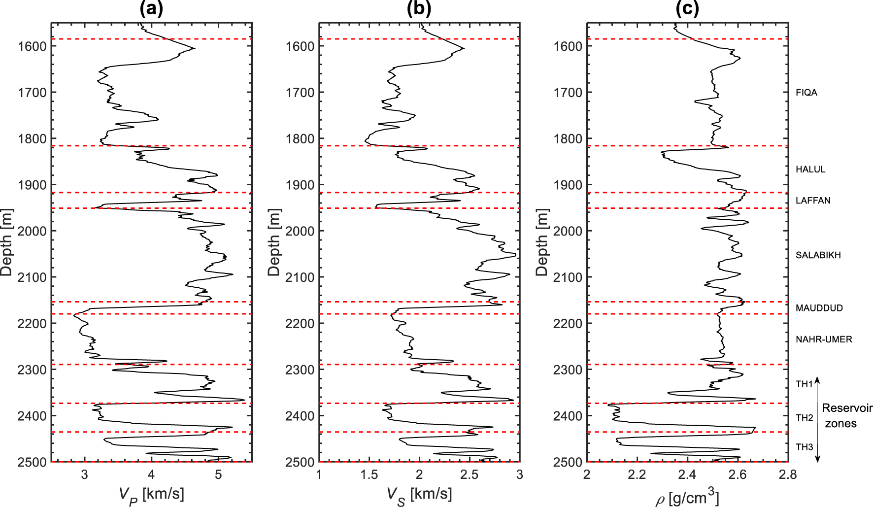
Particle motion of waveforms extracted around the time indicated by the dashed curves in Figure 5. The waveforms are aligned in the direction of L, Q, and T, the components of a ray-based coordinate system which are aligned with P, SV, and SH phase motions. The waveforms are recorded at a depth of 2305 m and an offset of 972 m.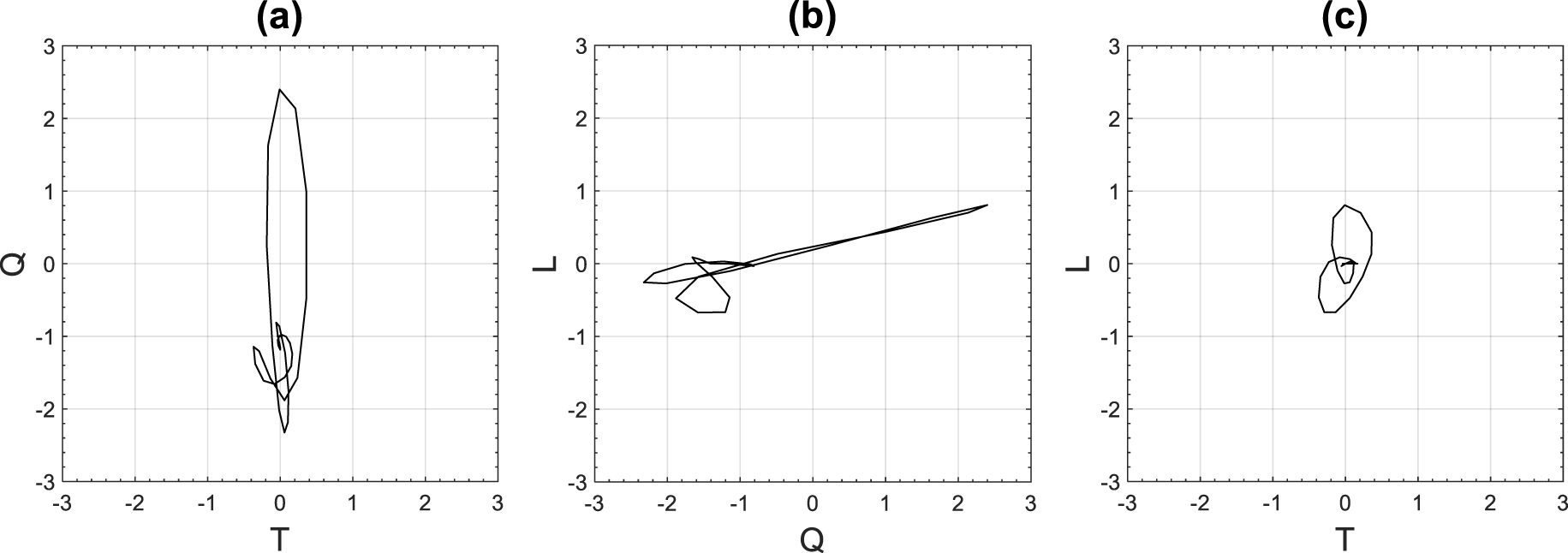
(a) Stacked S waveforms and (b) P waveforms recorded in the offset range of 817–1218 m at the top and bottom of each formation and reservoir zones. The P and S waveforms were extracted by using a Hann window of 60 ms and 70 ms, respectively.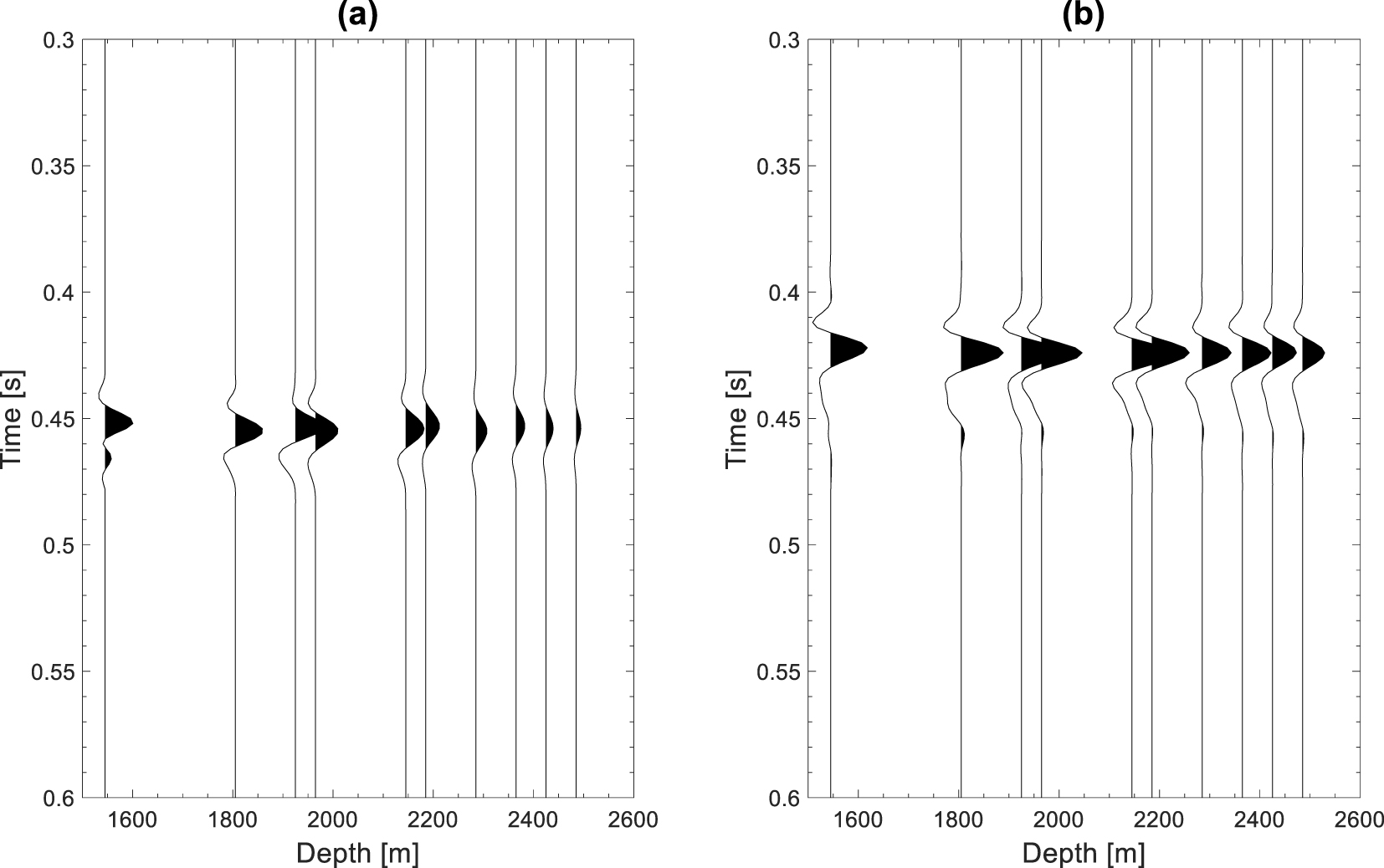
Curves of normalized amplitude of the spectral ratio versus frequency of the best (a, c) and the worst (b, d) linear regression for P waves (upper row) and S waves (lower row). The dashed lines represent the linear regression lines.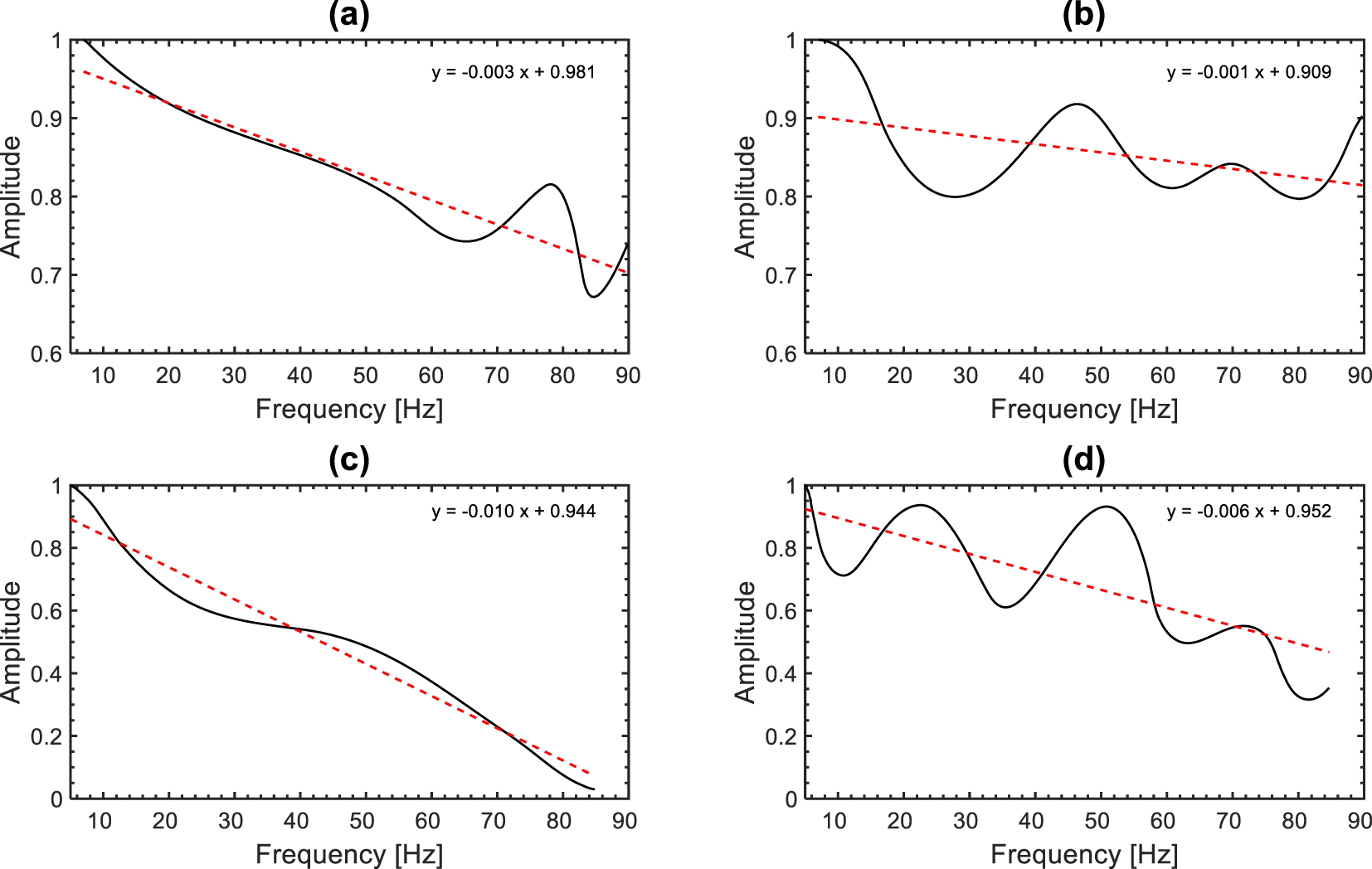
We aligned traces recorded in the offset range of 817–1218 m by using the simulated travel times. Then, an automatic picking of amplitude maxima was performed to refine the alignment, before stacking the traces in order to increase the SNR and hence, to facilitate the extraction of the downgoing S waves. A Hanning window with a length of 70 ms was chosen to extract the S waves (Figure 8a). In addition to S waves, we also extracted the first arrival of downgoing P waves, which are easily identifiable by their high amplitudes (Figures 3a–c). A Hanning window with a length of 60 ms was used to extract P waves (Figure 8b).
We estimated seismic wave attenuation in each formation by using the extracted waveforms of each two receivers located at the top and the bottom of each formation and reservoir zones. The spectral ratio method [Bath 1974; McDonal et al. 1958] was applied to estimate seismic wave attenuation from the extracted downgoing waves. In this method, a linear regression is performed between the logarithmic ratio in the left-hand side of (1) and frequency f.
| (1) |
| (2) |
After applying the spectral ratio method in specific intervals of the full frequency ranges, we noticed that the profiles with the most reasonable magnitudes (less than 1 and mostly positive) and the best linear regression were obtained in the frequency ranges of 7–90 Hz and 5–85 Hz for P and S waves, respectively (Figures 9 and 16). The standard errors (SE) of the linear regressions are in the range of 0.0023–0.0024 and 0.0025–0.0036 for P and S waves, respectively (Figure 10a). The larger SE error magnitudes of S waves was expected because of the difficulty in extracting S waveforms compared to P waveforms. The magnitudes vary from −0.034 to 0.135 (Figure 10b), while the magnitudes vary from 0.015 to 0.173 (Figure 10c). The magnitudes of are globally larger than those of except in the reservoir zones.
(a) Standard error (SE) of the linear regression of the spectral ratio versus frequency curves as a function of depth for P waves (black) and S waves (blue) in the frequency ranges 7–90 Hz and 5–85 Hz, respectively. (b) and (c) Profiles of total attenuation (solid lines) and scattering component (dashed lines) in the frequency ranges 7–90 Hz and 5–85 Hz, respectively. (d) Relative variation of the retained P (black) and S (blue) sonic velocities, which are averaged in each formation. The horizontal dashed lines and the text labels indicate the tops and names of the various formations.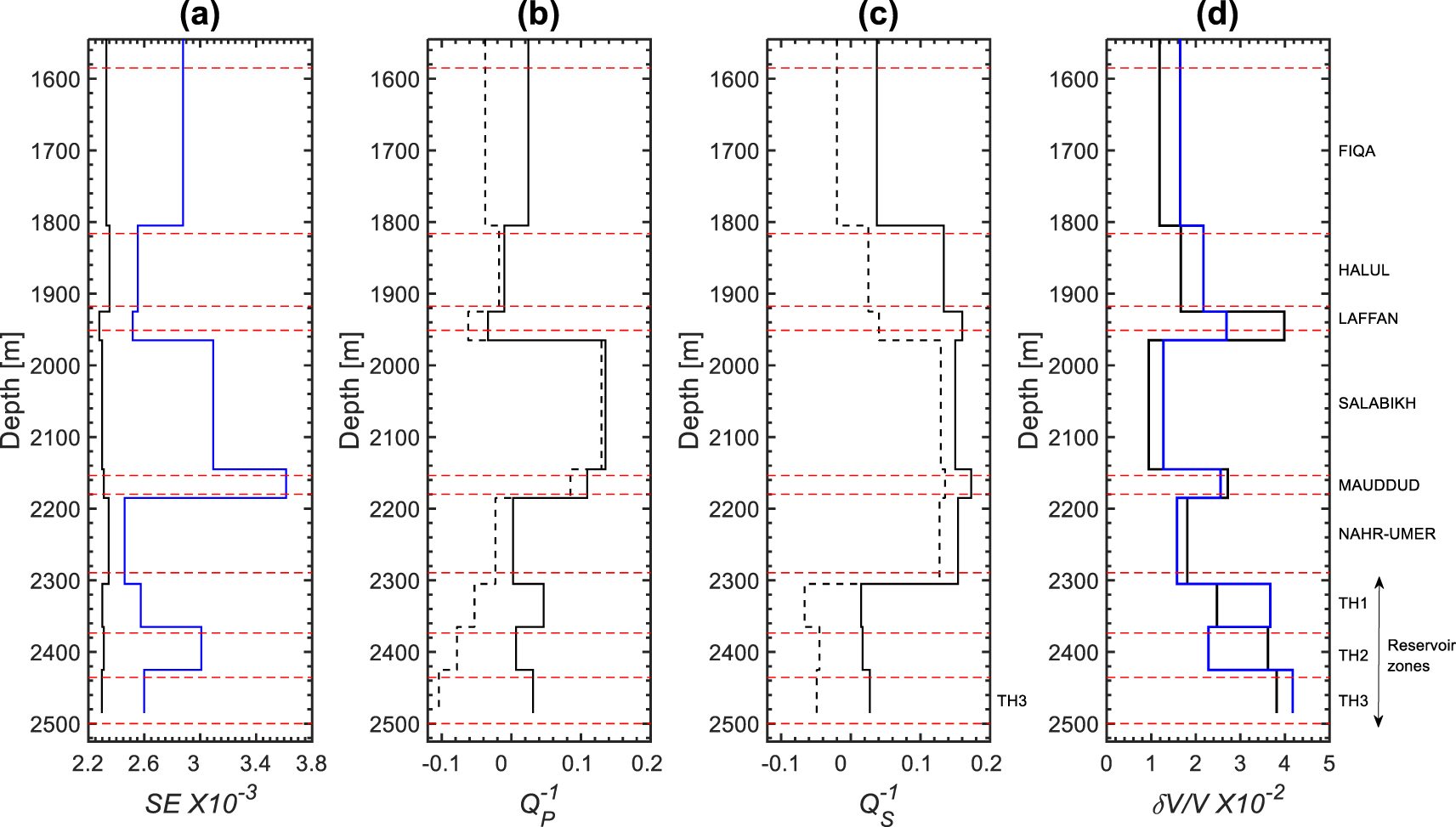
The Wasia Group, which consist of Salabikh, Mauddud, and Nahr-Umer Formations, displays the highest attenuation magnitudes. The Thamama reservoir zones (TH1, TH2, and TH3) display attenuation magnitudes lower than those of Wasia Group as in Figures 10a and c, even though these reservoir zones contain fluids and consequently attenuation is expected to be high. This is explained by the fact that the estimated attenuation is a combination of the intrinsic attenuation and scattering . The latter is an elastic phenomenon, which quantifies the losses due to small reflections caused by the heterogeneity of the subsurface formations. Therefore, to investigate the link between pore fluids and attenuation, component should be removed from Q−1, which is usually referred to as total attenuation. Schoenberger and Levin [1974] expressed Q−1 as follows:
| (3) |
Therefore, based on (3) and profiles can be separately estimated by calculating first, then subtracting it from Q−1 to obtain .
Scattering was estimated by applying the spectral ratio method on synthetic seismograms generated from the convolution of the reflectivity with a unit spike as an input source wavelet. The reflectivity of the medium was obtained by using Goupillaud model [Goupillaud 1961], which expresses the relationship between reflected and transmitted responses at the top (Rk,Tk) and the bottom (Rk+1,Tk+1) of the kth layer as
| (4) |
A band pass filter was applied on the synthetic seismograms in order to estimate in the same frequency range used to estimate (7–90 Hz) and (5–85 Hz). The compressional () and shear () scattering profiles display magnitudes ranging from −0.104 to 0.123 and from −0.066 to 0.135, respectively (Figures 10b and c). Scattering magnitudes are significant, which is in agreement with the high variation of velocity with depth (Figure 10d).
Following (3), the profiles were obtained after subtracting from Q profiles. The P and S intrinsic attenuation magnitudes vary from 0.009 to 0.135 and from 0.021 to 0.12, respectively (Figures 11a and b). Overall, the and profiles exhibit similar variation, except in Halul Formation where has higher magnitude than that of . The highest magnitudes of and are noticed in the reservoir zones and Halul Formation, respectively. The magnitudes of ratio is higher than 1 in the reservoir zones, while it is less than 1 in almost all of the other shallow formations (Figure 11c). Moreover, the ratio shows a good correlation with the resistivity profile in the reservoir zones (Figures 11d and e).
(a) and (b) VSP intrinsic attenuation profiles of P and S waves in the frequency ranges 7–90 Hz and 5–85 Hz, respectively. (c) P to S VSP intrinsic attenuation ratio as a function of depth. (d) P to S attenuation ratio profile in the reservoir. (e) Resistivity log averaged between receivers located at the top and the bottom of each reservoir zone. The dashed lines and the text labels indicate the tops and names of the reservoir zones.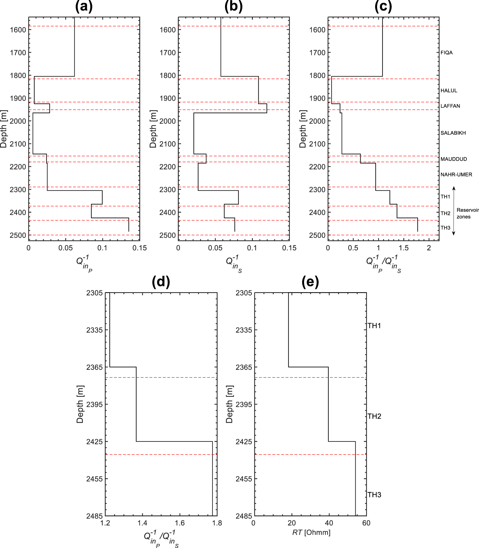
4. Estimation of sonic attenuation
Frazer et al. [1997] developed the median frequency shift (MFS) method to estimate attenuation from sonic waveforms. The MFS method is based on the following relationship between the median of frequency shift and the attenuation Q−1(z),
| (5) |
| (6) |
Hence, the values of are relative and strongly dependent on the arbitrarily reference value Q−1(𝜉). Suzuki and Matsushima [2013] significantly reduced the arbitrariness in Q−1(z) estimate, by suggesting a linear fitting of over 𝛥t(z) to define the reference value Q−1(𝜉). They refer to the corrected MFS method as modified mean frequency shift (MMFS) method. We use the MMFS method to estimate Q−1 from the sonic waveforms of this study.
Bouchaala et al. [2016a] showed that the scattering estimated in carbonate rocks at sonic frequencies is insignificant. They suggested that this might be due to the spatial sampling of sonic logging data, which is not sufficient to catch the heterogeneities that affect sonic waves. Therefore, we consider the sonic attenuation profiles as being representative of the intrinsic attenuation. The magnitudes of compressional attenuation and shear attenuation are in the range of 0.06–0.120 and 0.034–0.085, respectively (Figures 12a and b). We notice that in the case of large (2294–2306 m) or zero (2348–2360 m and below 2370 m) clay content (Figure 12d), attenuation is relatively low while in the case of small or moderate amount of clay (2306–2348 m and 2360–2370 m) (Figure 12d), attenuation is relatively high (Figures 12a and b). As in the VSP case, the ratio is larger than 1 (Figure 12c). The cross-plots of sonic attenuations with water content (𝛷 = the product of porosity and water saturation) show a clear decrease of and with increasing 𝛷 and increase of and with increasing resistivity (Figures 13a and b).
Attenuation profiles of (a) Monopole (compressional), (b) dipole (shear), and (c) monopole to dipole ratio (continuous curves) and their VSP counterparts (dashed lines) attenuation profiles. (d) Clay content in the reservoir zones. VCL is the fractional volume of clay. The horizontal dashed lines indicate the top and base of the reservoir TH1 zone.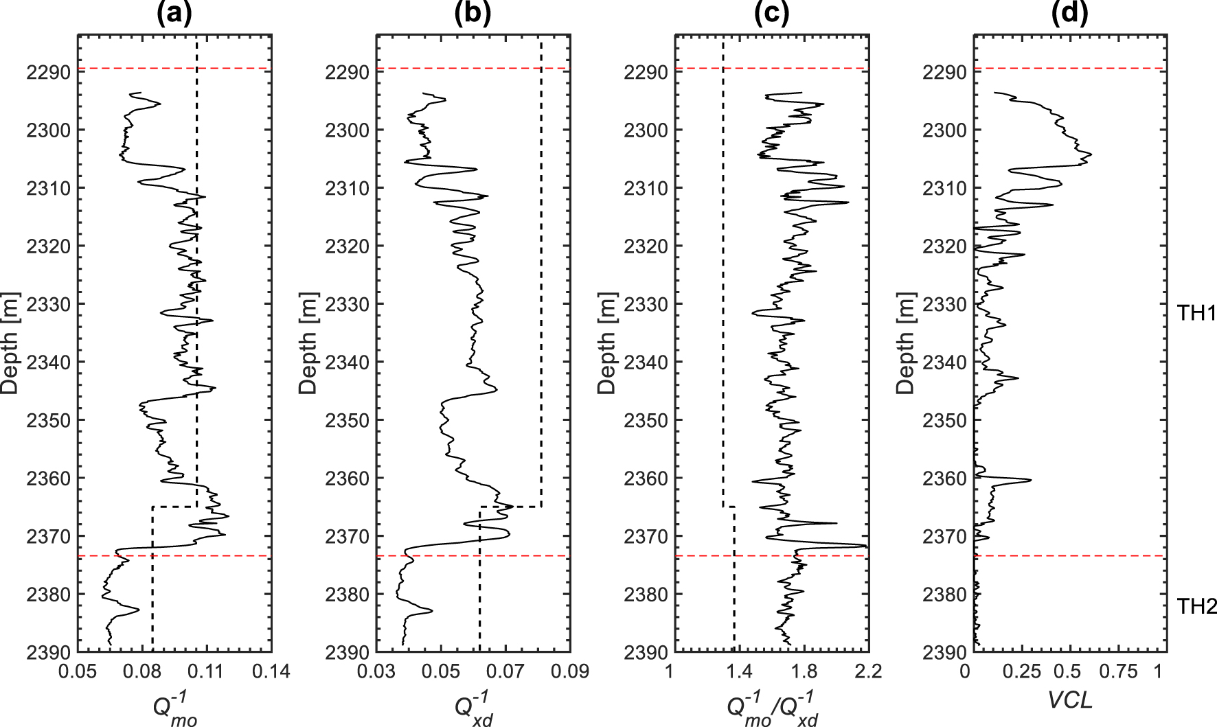
Cross-plots of (a) monopole, (b) dipole, and (c) monopole to dipole attenuations versus water content (𝛷 = porosity ∗ water saturation), color-coded by resistivity (RT).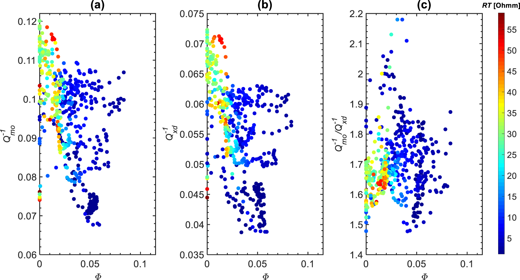
5. Discussion
5.1. Correlation between attenuation and petrophysical properties
After a careful extraction of downgoing P and S waves, we were able to estimate their corresponding attenuations. The high scattering magnitudes observed in various formations (Figures 10b and c) confirm the heterogeneous nature of the oilfield’s subsurface geology. This is consistent with the high variation of velocity (Figure 10d), and opposed to most attenuation studies carried out in sandstones where scattering is usually reported insignificant [e.g., Matsushima and Zhan 2020; Pevzner et al. 2013]. However, negative magnitudes of were noticed, particularly in the reservoir zones (Figures 10b and c). Liner [2014] suggested that a negative scattering is the result of a negative impedance contrast which implies a negative normal reflection coefficient (R0). Therefore, based on the partitioning relationship for seismic displacements R0 + T0 = 1, the normal transmission coefficient (T0) has to be larger than 1, meaning an amplification in the amplitude of transmitted waves which results in negative . Consequently, the negative magnitudes of in the reservoir zones may be due to negative impedance variations (Figure 6) caused by high porosity and fluid content. Mateeva showed that in finely layered medium, primary reflections overlain or underlain weak reflections, which leads to negative attenuation. Furthermore, Gist [1994] suggested that for a proper estimate of scattering, 3D heterogeneities should be taken into account. Therefore, as suggested by Bouchaala et al. [2016a], the interference of small reflections with primaries in the vicinity of receivers and the neglect of 3D heterogeneity in scattering estimation might imply negative magnitudes of .
Hassan and Azer [1985] reported a small accumulation of heavy oil in Halul Formation in the northern Abu Dhabi offshore, where the study area is located. The decrease in sonic velocities and density in the depth range of 1840–1880 m might be related to the presence of heavy oil (Figure 6). Batzle et al. [2006] pointed out the strong frequency dependence of shear modulus on heavy oil-saturated rocks, which means high shear attenuation. The relative frictional motion between solid grains and heavy oil which behaves as a solid during the wave passage due to its high viscosity might be the cause of high shear attenuation Hamilton [1972], Mavko and Nur [1979]. This is in agreement with the highest magnitude of noticed in Halul Formation, if the assumption of heavy oil content is verified. Furthermore, the highest magnitudes noticed in the reservoir zones are most probably due to fluid-related mechanisms, which mainly affect P waves.
Due to limitations in the quality of sonic waveforms, the sonic attenuation was estimated in the reservoir zone TH1 and the upper part of reservoir zone TH2 only. The notable changes of sonic attenuation with the variation of clay content (Figure 12), might be due to the effect of clay on the permeability, which controls the fluid flow and hence the intensity of attenuation mechanisms. The oil content is usually negatively correlated to water content (𝛷) and directly proportional to resistivity (RT). Therefore, the clear decay of and with 𝛷, and their highest magnitudes at high RT areas (Figures 13a and b), suggests a good correlation with oil content. The oil trapped in this reservoir ranges from medium to light Hassan and Azer [1985]. Therefore, it behaves as a fluid during the wave passage and not as a solid as it is the case of heavy oil. Consequently, as for the VSP case, the increase of sonic attenuation with oil content is most probably due to fluid-related mechanisms, which manifest themselves through the frictional movement between pore fluids and grain solids.
5.2. The compressional to shear attenuation ratio in the reservoir zones
The highest magnitudes of noticed in the reservoir zones (Figure 11c) are most likely caused by the high fluid content. As explained above for and , the good correlation between and the resistivity profiles in the reservoir zones (Figures 11d and e) suggests that the magnitude of is directly related to oil saturation. The ratio shows an increase with Poisson’s ratio (𝜈). This increase is confirmed with two distinct models proposed by Dvorkin et al. [2014] for wet sediments, which show an increase of with 𝜈, and which predict magnitudes between 1 and 3 in the Poisson’s ratio interval 0.30–0.35 (Figure 14). However, none of the theoretical models (7) and (8) satisfactorily matches the estimated value.
| (7) |
| (8) |
| (9) |
| (10) |
| (11) |
The reservoir zones, which are fully saturated with oil and water, display and magnitudes larger than 1 (Figures 11d, 12c, and 13c). This is in agreement with the observations of Adam et al. [2009] who experimentally investigated seismic wave attenuation in fully and partially saturated carbonate core plug samples acquired from one of Abu Dhabi reservoirs. However, shear attenuation is mostly observed to be greater than the compressional attenuation in fully saturated sandstones [e.g., Best et al. 1994; Murphy 1982; Winkler and Nur 1982]. To understand the contradiction between the two observations, it should be pointed out that the interpretation of the magnitude of compressional to shear attenuation in partially and fully saturated sandstones is based on a rock physics model assuming that fluid flows between two identical low aspect ratio cracks and orthogonal at their tips [Winkler and Nur 1982]. This conceptual model is too simple and not adequate for carbonate rocks known for their complex texture. Therefore, the degree of fluid saturation is not the unique parameter which controls the magnitude of attenuation ratio in carbonate rocks.
Cross-plot of monopole to dipole attenuation versus Poisson’s ratio (𝜈), color-coded by water content (𝛷 = porosity ∗ water saturation). The blue and black dashed curves were produced from (7) and (8), respectively.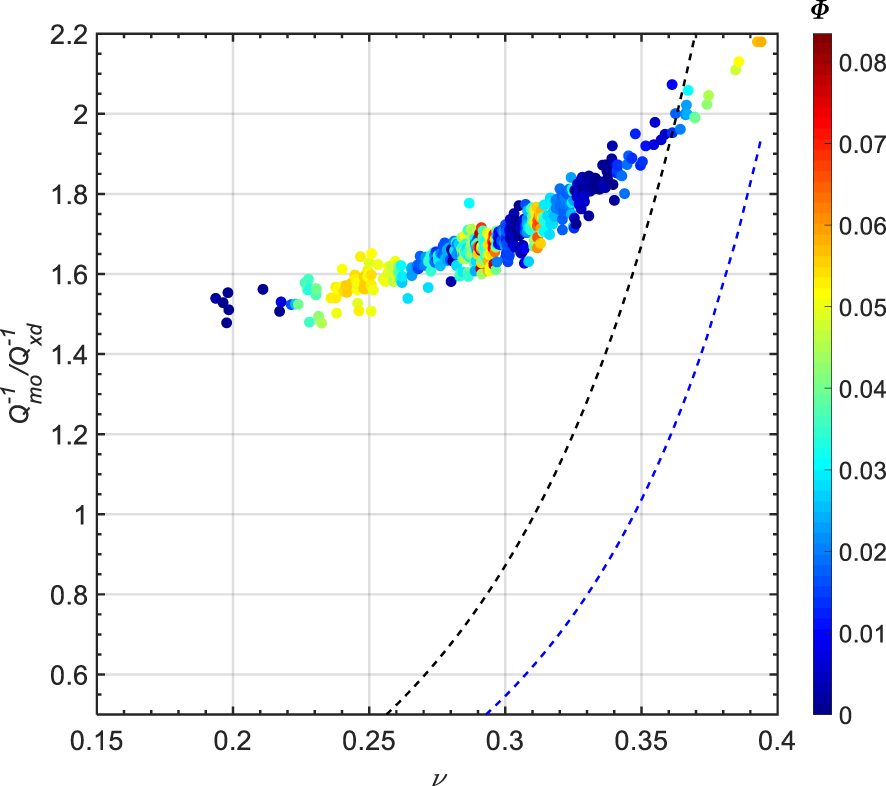
5.3. Frequency dependence and attenuation mechanisms
The attenuation magnitudes at sonic and VSP frequencies are of the same order (Figures 11a, b, 12a and b). This suggests frequency-independent attenuations in this oilfield. Moreover, compressional and shear attenuations show similar variation in both frequency ranges (Figures 12a and b). The positive correlation of attenuation magnitudes with resistivity and its negative correlation with water content, implies a positive correlation between attenuation and oil. Therefore, we suggest that the fluid-related mechanisms such as global and squirt flow mechanisms [e.g., Müller et al. 2010; Murphy et al. 1986] caused by the oil at VSP frequencies, induce a higher increase in the compressional attenuation than in the shear attenuation. Klimentos [1995] assumes that during the wave passage, the compliant pores located between clay (soft material) face higher deformation than stiff pores located between carbonate grains (hard material), which results in the squeezing of the fluid contained in compliant pores. Consequently, the fluid flows toward stiff pores with high speed, which causes high frictional losses known as by the squirt flow mechanism. Accordingly, squirt flow mechanism is weak in media with very low amount of clay or with high amount of clay. This may explain the higher sonic attenuation in the zone with moderate clay content than the zones with high or no clay content (Figure 12).
Illustration of Dipole Sonic Imager (DSI) tool, used to acquire the sonic data.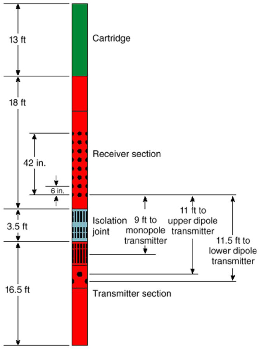
VSP attenuation profiles of (a) P waves and (b) S waves as function of depth estimated in different frequency ranges and their corresponding standard errors (c and d).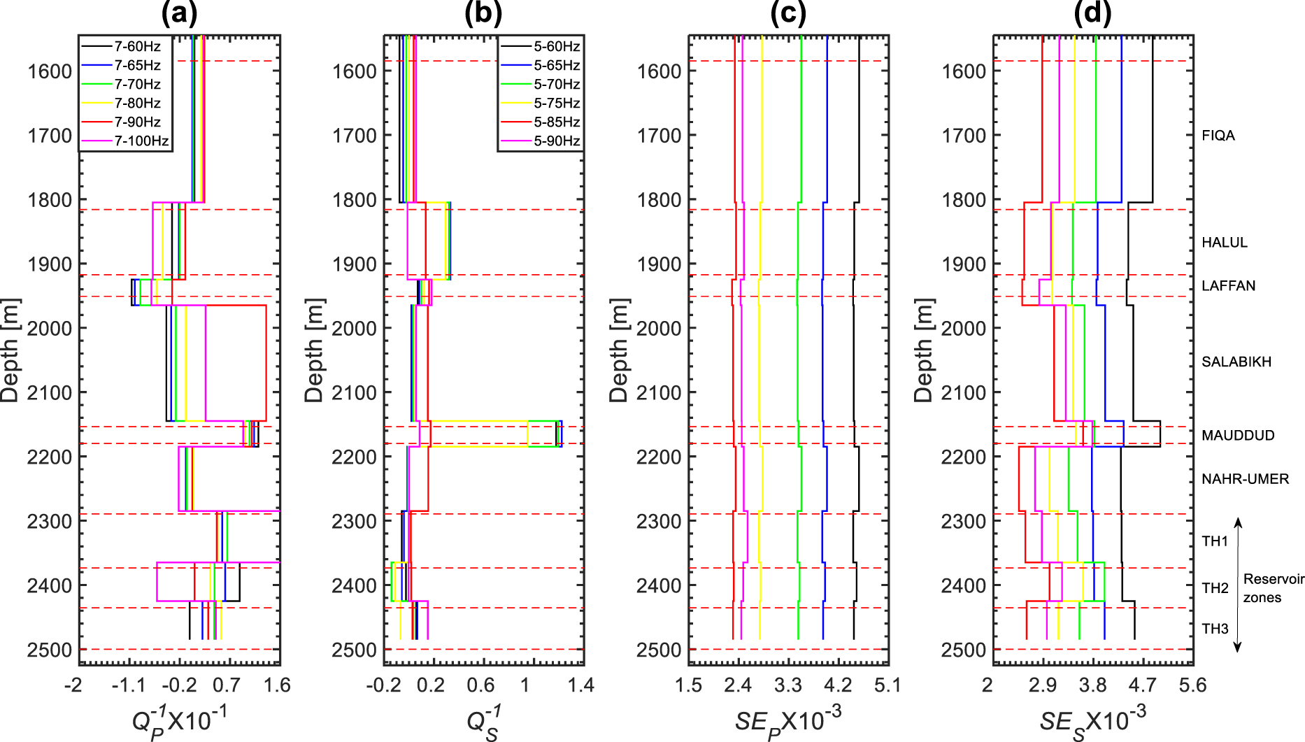
6. Conclusions
We investigated the link between petrophysical properties of carbonate rocks and attenuation estimated from downgoing P and S waveforms carefully extracted from 3D VSP and sonic data. The elevated magnitudes of scattering at VSP frequencies confirms the highly heterogeneous and complex nature of carbonate rocks. The high magnitudes of and ratio indicate oil-rich zones, while high shear attenuation indicates a heavy oil zone. At sonic scale, both and show high sensitivity to oil content through their high magnitudes in high resistivity and low water content zones. Furthermore, clay content also controls the magnitude of attenuation through squirt flow mechanism, which is strong at moderate amount of clay. The higher than 1 magnitude of compressional to shear attenuations in the reservoir zones confirms the previous experimental results carried out on fully saturated carbonate samples, and suggests the non-validity of sandstones attenuation models for carbonate rocks.
Acknowledgment
We would like to thank the Abu Dhabi National Oil Company (ADNOC) for the financial support of this project and for permission to use the data used in this project.
Appendix A The wavefield separation method, Wavesip [Leaney 2002]
This technique is applied on 3C VSP data rotated to the geographical coordinate system (Easting, Northing, and Vertical). The data are then converted to the frequency domain by applying the Fourier transform in order to obtain the linear system below at each frequency,
| (A1) |
For an array of M 3C geophones, the matrix G has N columns and 3M rows, each element of the matrix is written as Pniei𝜔(Sn⋅Dm), where Pni(i=1,2,3) is a component of the polarization vector and Sn is the slowness vector of each plane-wave n (qP, qSv, or Sh), respectively, and Dm is the coordinate of the mth receiver in the geographical system.
Slowness and polarization vectors are computed for each plane wave to solve the linear system in (.1), at each frequency to yield the plane-wave amplitudes and hence, to decompose the data into an angular spectrum of plane waves. In our case, the five parameter inversion simplex method [Leaney 2000] was used to estimate qP and qSv slowness and polarization. Eventually, the decomposed plane waves are summed by type into downgoing qP, upgoing qP, downgoing qSv, and upgoing qSv wavefields.