

1 Introduction
In recent years, the widespread implementation of sophisticated new technologies in the field of functional brain imaging has given rise to a revival in research devoted to the topography of human brain activity during sleep. For instance, using very short half-life isotope (oxygen-15) and powerful three-dimensional statistical techniques, positron emission tomography (PET) studies have yielded original data on the functional neuroanatomy of human sleep (reviewed in 〚1〛). Recent advances in functional magnetic resonance imaging (fMRI) techniques will soon allow even more precise description of the spatio-temporal brain activities and regional interactions during sleep. Thus, Lövblad et al. 〚2〛 recently showed selective activation or deactivation of specific brain areas in rapid eye movement (REM) sleep using silent sequences (allowing the subject to sleep during echo-planar acquisitions) and new device allowing the acquisition of electrophysiological signals in the magnetic field.
It has however to be kept in mind that both aforementioned PET and fMRI techniques are measuring regional cerebral blood flow (rCBF), an indirect marker of neuronal activity. For instance, in certain circumstances, neurogenic control of local CBF, due to the presence of nerve fibres in the vicinity of cerebral vessels, would alter the link between neuronal activity and rCBF 〚1〛. In this regard, registration of topographic properties of EEG sleep signals could provide additional information that could complement rCBF data. It has been shown that sleep EEG activity is not a homogenous global phenomenon and that regional differences of EEG frequency band depend on sleep stage and cortical area 〚3–10〛. More recently, magnetoencephalography (MEG) signals have been used for source localisation during sleep 〚11, 12〛. The advantage of MEG over EEG in source localisation is due to the fact that MEG is mainly sensitive to primary currents, and not as sensitive as EEG to conductivity changes, which results in a better spatial accuracy. But there are limitations in using MEG, one reason being that the type assessment is, as yet, not very accessible for clinicians; moreover, due to the discomfort of staying in a fixed position, very few subjects are able to remain for a period long enough to enter various sleep stages (deep and paradoxical sleep stages for example). We have been seeking for a more versatile approach and multi-electrode EEG recording seems to be more appropriate to study all night sleep. Both MEG and EEG source modelling rely on a discrete number of dipoles, and, most of the time, source identification in sleep research concerns transient physiological signals (k-complexes for example), and only a very limited number of potential dipoles are taken into account 〚11, 12〛. Maquet and Phillips 〚13〛 suggested however that techniques using distributed solutions where each voxel is a possible current source, such as the low-resolution electromagnetic tomography (LORETA) method 〚14〛, are probably more suitable for obtaining three-dimensional measurements of the brain activity during sleep.
In this paper, we deal with EEG source estimation (LORETA) averaged for long time series associated with different steady states during sleep. Moreover, we present a methodology to compute an EEG source estimation related to a given frequency band.
2 Materials and methods
2.1 EEG source estimation
In a general way, the EEG source estimation must be regarded as an inverse problem. By way of a scalp-montage, surface electrical fields are recorded continuously. These fields are mainly generated by the cortical pyramidal cells that can be considered as sources of current, and called elementary dipoles. The pyramidal cells are situated in the grey matter of the brain. The EEG source estimation problem consists of calculating the position and the orientation (three coordinates) of these elementary dipoles from the distribution of scalp potentials.
A large number of mathematical approaches can be used for computation, but every method needs explicit or implicit assumptions about the physical properties and geometrical configuration of the pyramidal cells in the brain. For example, a specific stimulus (auditory, visual, etc.) usually causes a significant change of the scalp electrical field that reflects the activation of pyramidal cells restricted to a small area in the grey matter (auditory cortex, etc.). So, the source estimation of these evoked potentials often assume that the electrical field is only generated by a single or a few dipoles. The difference between the electrical field approximation on the basis of this assumption and the actual experimental electrical field is attributed to unknown sources or recording noise.
With regard to a study during a long period of time (several minutes), thousands or more pyramidal cells contribute to the electrical fields and the mathematical approach must take into account a wide distribution of dipoles. In this point of view, the LORETA algorithm developed by Pascual-Marqui uses 2394 dipoles evenly distributed in the grey matter. For an elementary dipole at a given position, we compute the contribution of its electrical field, including its three moments at each electrode of the array. The head is modelled by homogenous conductive sphere (brain) surrounded by inner (skull) and outer (scalp) shells of differing conductivity (three sphere model). Then, an exact mathematical expression 〚15, 16〛 gives the lumped electrical influence on each electrode of dipoles located inside the first sphere (brain). Consequently, a linear formalism between the 2394 dipoles and the 21-electrode network (Fp1, Fpz, Fp2, F7, F3, Fz, F4, F8, T3, C3, Cz, C4, T4, T5, P3, Pz, P4, T6, O1,Oz, O2 in the standard 10–20 system, see 〚17〛) can be established:
As a standard head model reference, LORETA makes use of the three-shell spherical head model registered to the Talairach human brain atlas 〚19〛, available as a digitised MRI from the Brain Imaging Centre, Montreal Neurological Institute. Topological adjustments of spherical model and realistic head geometry use EEG electrode coordinates reported by Towle et al. 〚20〛.
In few words, LORETA method computes an estimation of the electrical activity distribution in the grey matter (standard anatomical head model) from the EEG cartographic recording (electrode array) of a subject.
This estimation is computed at each sample point and provides an instantaneous representation of cerebral activity. According to this short theoretical presentation, LORETA method seems very appropriate with evoked potential (transient EEG reactions) studies to monitor information processing. More, evoked potentials are usually characterised by a high signal to noise ratio that leads to very favourable conditions for LORETA method application. Nevertheless, we are going to show that, with take of precautions, LORETA is a very interesting tool to study long-term and spontaneous EEG activity too.
2.2 Frequency approach
For sleep analysis, the all-night cerebral activity is most of time described as a series of sleep stages (deep sleep, light sleep, awake, paradoxical sleep, etc.). Each sleep stage presumably corresponds to a fundamental behavioural state that can be classified by the spectral composition of the EEG signals. For example, a decrease of vigilance (awareness) is associated with a rise of low frequency components of the EEG signal. In a simplified way, the EEG signal during sleep, may be split up in four frequency bands: δ 0.5–3.5 Hz (low frequencies), θ 4.0–7.5 Hz and α 8.0–12.5 Hz (medium frequencies), β 13.0–32.0 Hz (high frequencies). By now many classical investigations have confirmed these frequency bands during sleep that have led researchers to build automated detection device to classify sleep 〚21〛. Moreover, on the one hand, the quantification by spectral power has been validated as a method for characterising pathologies and pharmacological effects. On the other hand, the combination between localisation methods and frequency analysis of the sleep EEG signals remains an unexplored domain.
Our methodological approach consists in selecting a period of time (several minutes) inside each continuous sleep stage. During this period, the EEG signal of each electrode (21 signal recordings sampled at 128 Hz) is processed with a pass band filter (a moving finite-duration window (2 s) and a fast Fourier transform). Next, we compute the LORETA distribution at each sample of this period, and finally a time average gives us estimation of the cerebral activity related to a frequency band. To make easier the comparison between different frequency bands, this average estimation has been normalised on the mean dipole amplitude (whole volume). The operation is repeated for each one of the four frequency bands given above.
At first sight, it might be thought that this filtering process provides us with a localisation image related to each frequency band. As a matter of fact, so obtained images are nearly the same: an important density in the central positions of the head that scatter in more occipital areas. An argument may be suggested to explain the similarity of the image pattern: the signal to noise ratio is low in the present case. The average localisation for a quite long time, emphasize the global influence of the white noise. In the LORETA method, a weight, inversely proportional to the gain that depends on the depth, is applied to each point source of the mesh. This leads to preferential solutions at the centre of the head in case of white noise. So, the previously obtained images are mainly due to the white noise, and, to a large extent, correspond to this weight distribution.
As a consequence, the frequency approach in itself does not lead to a relevant imaging methodology. To solve this fundamental problem, we advocate a relative imaging methodology. In concrete terms, to point out the specificity of each frequential normalised average distribution, we compare these distributions with the normalised average distribution for the full frequency band (0.5–32.0 Hz). And the computation for each band of the relative density consists in the difference of each estimated dipole amplitude with regard to this full frequency distribution: (band–full)/full.
To sum up, this method gives an estimation of the regional relative cerebral activity associated with a frequency band during a determined EEG condition for each individual subject.
2.3 Statistical validation
A lack of contribution for a particular frequency to the cerebral activity results in a relative difference that equals zero. So, comparisons to test null hypothesis (t-values), i.e., that this relative difference equals zero, have been carried out for each voxel. For each frequency band, the global three-dimensional distribution of the voxel-by-voxel t-values was visualised in a Talairach human brain atlas. The red and blue colour corresponds to positive and negative differences from the full spectrum, respectively. Comparisons between sleep stages are made in a qualitative way, and only obvious differences by visual inspection are described.
2.4 Recording procedure
The recording study population was a group of 19 young male (mean age: 25.8 years, SD = 6.6) healthy volunteers. After one habituation night, the all-night sleep of each subject was recorded from a 28-electrode array: using a common linked-ear reference. The electronic device used for amplification and analogue filtering (type: Bessel order 2) was adjusted to 0.5–32 Hz as cut-off frequencies. The EEG signals were digitised at a sampling rate of 128 Hz. Afterwards, each all-night recording was analysed and, for each 30 s epoch, the sleep stage was visually identified, according to Rechtschaffen et Kales, by at least two confirmed scorers. Then, 21 EEG electrodes were selected and our frequency approach in source localisation was applied to periods of 20 consecutive epochs of paradoxical sleep (REM sleep), deep sleep (slow wave sleep) and light sleep (stage 2). For the display of the so-obtained three-dimensional distributions in the Talairach atlas, the LORETA–KEY software, developed by R.D. Pascual-Marqui, was used. Results are shown in the three orthogonal brain views, sliced at the level of the region of the maximum positive t-value.
3 Results
3.1 Paradoxical sleep (REM sleep)
For each subject, the epoch of 10 continuous minutes of paradoxical sleep was selected at the end of the night, during the fourth REM–non REM cycle. The results are shown in Fig. 1; it can be noticed that, in a general way (cf. Figs. 2 and 3), generators for the low frequency activity (δ-band) are localised in anterior regions, and higher frequency activity (θ-, α- and β-bands) in more posterior regions.
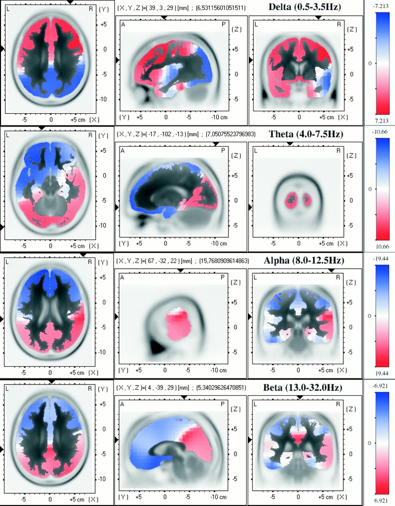
Paradoxical sleep (REM sleep). Images of voxel-by-voxel t-statistics of brain regional electrical activity for four frequency bands. The structural anatomy is shown in grey scale (white-to-black). Left: axial slices, seen from above, nose up; centre: sagittal slices, seen from the left; right: coronal slices, seen from the rear. The location of the maximal t-value is graphically indicated by black triangles on the coordinates axes.
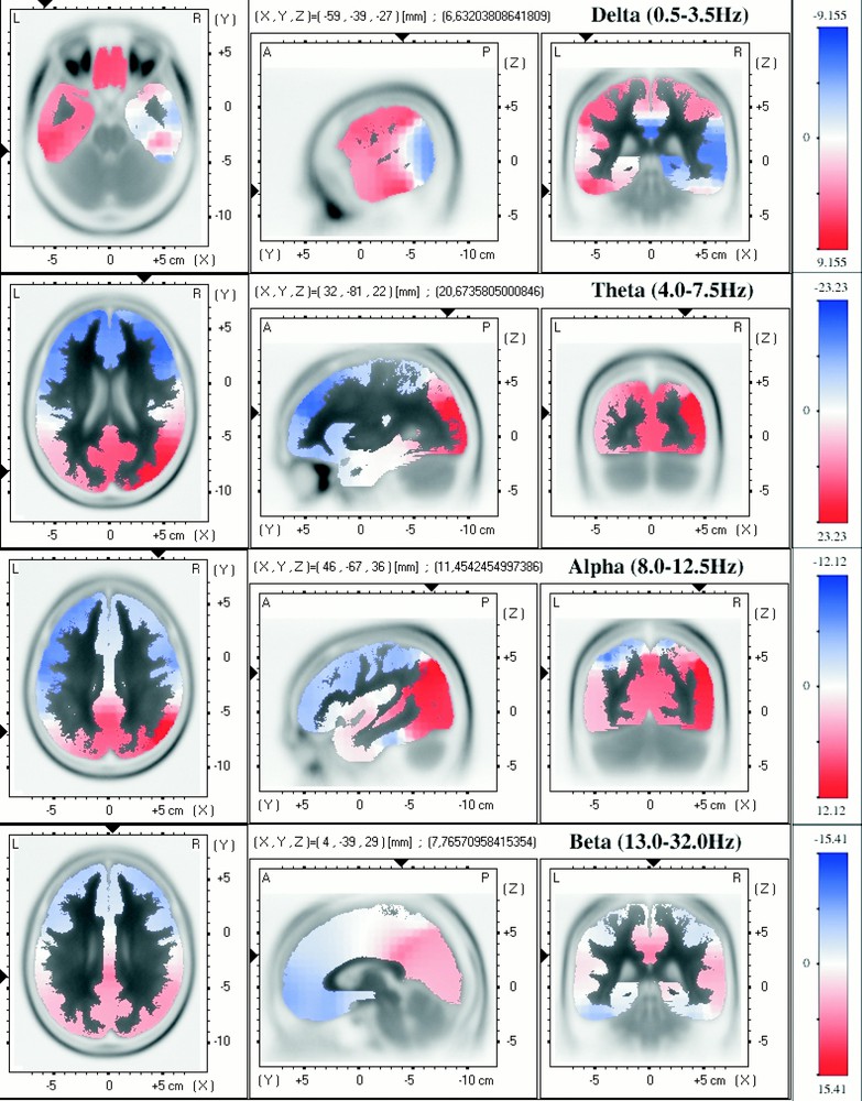
Deep sleep (slow wave sleep). For details, see legend of Fig. 1.
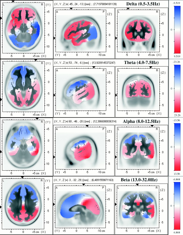
Light sleep (stage 2). For details, see legend of Fig. 1.
δ-Band relative activity is located predominantly in the superior frontal lobe and more pronounced in the motor cortex. For θ- and α-bands, an obvious asymmetry between right and left hemisphere can be observed. The relative source-activity of θ-band is important in both sides of the occipital part of the brain (visual cortex), but a relative positive contribution is observed in the right temporal lobe, whereas the relative activity is negative in the left temporal lobe. In the same way, the relative influence of the alpha band is far more important in the right temporal lobe.
With regard to the β-band activity, the distribution seems more central and the maximum is located in the region of posterior cingulate gyrus.
3.2 Deep sleep (slow wave sleep)
The three-dimensional distribution of relative activity for each frequency band during 10 min of continuous slow wave sleep (either stage 3 or stage 4) in the first REM–non-REM cycle is shown in Fig. 2. For the δ-band, we can notice that the superior frontal lobe is far less important, and the maximum of the relative activity is localised predominantly in the left anterior inferior temporal lobe. Concerning θ and α frequency bands, the relative activity is important in the right parietal and occipital lobes. The localisation of the cerebral activity for the β-band does not seem to be fundamentally different from that for the paradoxical sleep period.
3.3 Light sleep (stage 2)
The third period of sleep that we explored consists of 10 min of continuous stage 2 sleep during either the second or the third REM–non REM cycle. From a global point of view, the distribution of the cerebral activity, related to light sleep, occupies an intermediate position between deep sleep and paradoxical sleep. For the δ-band, the most abundant relative activity is found in the left inferior frontal lobe (Fig. 3). For the θ-activity, the distribution of positive and negative areas is not very different from that for paradoxical sleep. The maximum, however, is observed in the right parietal and occipital lobes (cf. deep sleep). Concerning α-band again, an asymmetry is present, with maximal cerebral activity in the right inferior posterior temporal lobe.
4 Discussion
As far as we are aware, this paper presents the frequency-dependent EEG source localisation related to sleep stages for the first time. In previous papers, generations of sleep rhythms were, most of time, interpreted on basis of the surface topographies of EEG recordings 〚22–28〛. In this article, we try to estimate the EEG sources, and the results can be compared with EEG mappings under acceptance of certain premises. The effect of an EEG source on the scalp potential depends on the position, the amplitude and the orientation of this current source. Due to its position and orientation, a high-intensity deep source can be difficult to detect from a direct recording of the EEG potentials. On the contrary, a weak source close by may have a greater influence on electrodes. Moreover, the observed EEG potential over the scalp results from a combination of several sources. So, three-dimensional source reconstruction must lead to a more realistic image than a simple mapping of the global effect over the scalp.
Nevertheless, some aspects of source localisation and EEG mapping can be compared. For example, the prevalence of the low frequencies in anterior brain regions and the higher frequencies in posterior positions, consistently shown in our figures, have already been described in many EEG mapping studies 〚9〛. About the low frequency distribution and sleep stage, Armitage et al. 〚23〛 affirm that δ-activity in slow wave sleep was more asymmetrical than in stage 2. Our study not only confirms these statements, but provides even more accurate information. In fact, we have noticed that the maximum of δ-activity during slow wave sleep was located in the left inferior temporal and in the left inferior frontal lobe during stage 2. So, this source localisation change involves a less asymmetrical EEG observation over the scalp during stage 2. Our analysis is in agreement with the suggestion Sekimoto et al. 〚25〛 that there exist distinct lateralities in the quantity of δ-waves in the central region, reflecting the functional asymmetry of the brain. Our three-dimensional analysis can be also confirmed by a MEG study 〚29〛, in which one subject reached a deep sleep stage. An important δ-activity was detected in the left temporal area during this sleep stage. In paradoxical sleep (Rapid Eye Movement Sleep), the localisation of the δ-power in the superior frontal cortex is most likely related to the ocular activity and is coherent with direct EEG and EOG traces. Concerning higher frequencies, we have noticed that α-activity was more significant in the right hemisphere, regardless of the sleep stages. In an EEG mapping study, Benca 〚28〛 also established a tendency for a rightward shift in α-power during sleep.
In summary, we find many points in common between our approach and EEG mapping investigations, but our methodology allows comparison with other three-dimensional physiological assessments too. If we assume that high frequencies (θ, α and β) result from an energy-consuming process and low frequencies (δ) from an economical process, we could fit activated areas for rCBF or magnetic resonance imaging methods (MRI) to those of high-frequency sources and deactivated areas to low-frequency sources. Our approach only considers localisation in the grey matter that renders results difficult to be fully compared to those obtained with rCBF or Magnetic Resonance Imaging. Despite fundamental difficulties, common observations can be made indeed. A MRI study of Lovblad and al. 〚2〛 proved that visual cortex is more activated during paradoxical sleep. This statement seems to be very consistent with the θ activity seen in Fig. 1. Similarly, the δ-activity observed in the temporal lobe during slow wave sleep seems to be in relation with the deactivation in some mesiotemporal cortical areas observed by Maquet 〚13〛 using an rCBF device.
5 Conclusion
The approach that we presented in this article constitutes a promising methodology to study the cerebral electrical activity. Based on EEG mapping recordings, our method is a low-cost and non-invasive technique that can be applied for a nearly unlimited period of time. The use of Fourier analysis of the electrical signal distinguishes the (possibly functional-relevant) activities in different frequency bands. In addition to classical EEG mapping methods, we report a three-dimensional way to analyse generators of the cerebral activity.
In fact, we showed that our method provides a very detailed description of physiological changes in neuroanatomical substrates that correlate to sleep during different stages; the interpretation is compatible to those derived on the basis of other techniques (classical EEG mapping, MRI, rCBF). As a consequence, this paper offers an argument in favour of the validation of the presented methodology as a tool for in-depth exploration of cerebral electromagnetic activity; the way is open for clinical applications in sleep disturbance or study of drug effects, for instance.
Acknowledgements
Our methodology is based on the inverse method called LORETA and on a LORETA–KEY software, developed by R.D. Pascual-Marqui. The authors are grateful to him for all the help that he gave us.
Version abrégée
Depuis quelques années, les nouvelles techniques exploratoires de l’activité cérébrale (imagerie fonctionnelle par résonance magnétique, tomographie par émission de positron, localisation numérique de sources EEG et MEG) apportent une connaissance tridimensionnelle plus précise du cerveau. Toutefois, les techniques classiques de cartographies EEG conservent l’avantage d’être peu contraignantes et de permettre une analyse fréquentielle. Ces dernières gardent donc une place privilégiée pour l’étude du sommeil. Nous avons cherché à intégrer les analyses en bandes de fréquences à une technique de localisation de source nommée Loreta (Low Resolution Tomography). Cette méthode de localisation a été développée par Pascual-Marqui. Elle repose sur une modélisation de l’influence des sources de courant sur les électrodes au niveau du scalp d’un sujet, et sur une technique d’inversion. Une source de courant, appelée dipôle et notée située dans une région précise du cerveau et dont les moments sont définis donne lieu à un champ électrique superficiel, mesuré par un réseau d’électrodes collées sur le scalp. Dans notre cas, nous avons considéré un réseau de 21 électrodes, situées à des positions standard sur de scalp (Fp1, Fpz, Fp2, F7, F3, Fz, F4, F8,T3,C3, Cz, C4, T4, T5,P3, Pz, P4, T6, O1,Oz, O2 dans le système 10–20 standard) et 2394 sources élémentaires réparties uniformément dans la matière grise du cerveau. Grâce à un modèle analytique où les différentes parties de la tête (cerveau, crâne, scalp) sont identifiées à des couches sphériques constituées de milieux à la conductivité connue, on calcule l’influence d’une source élémentaire sur chacune des électrodes. Le potentiel électrique global observé au niveau du scalp sera supposé être la somme de chacune des contributions élémentaires. Ainsi, entre les moments des dipôles et les valeurs du potentiel électrique mesuré par les électrodes, on construit une relation linéaire :
Nous avons appliqué notre méthode originale à l’étude du sommeil chez un groupe de 19 jeunes adultes mâles. Trois périodes de 10 min ont été sélectionnées : une période de sommeil paradoxal (REM sleep) en fin de nuit (4e cycle REM–non REM), une période de sommeil profond (stade 3 ou 4) en début de nuit (1er cycle) et une période de sommeil léger (stade 2) en milieu de nuit (2e ou 3e cycle). La période de sommeil paradoxal s’est caractérisée par une activité δ relativement plus importante dans les lobes frontaux supérieurs, voire même dans le cortex moteur. De même, pour la bande de fréquence θ, une activité spécifique a pu être remarquée des deux côtés de la partie occipitale du cerveau (cortex visuel). La période de sommeil profond (stade 3 et 4), quant à elle, s’est distinguée par une activité relative prédominante dans le lobe temporal gauche inférieur, les lobes frontaux supérieurs jouant un rôle moindre. Nous avons également pu remarquer des activités α et θ plus postérieures que celle observée lors du sommeil paradoxal. Lors de la période de sommeil léger (stade 2), les distributions tridimensionnelles de l’activité cérébrale semblaient être intermédiaires entre celles obtenues pour le sommeil paradoxal et le sommeil profond. Enfin, nous avons pu établir que, pour toutes les périodes, l’activité β se localisait principalement dans la région du gyrus cingulaire postérieur. De même, la bande de fréquence δ semblait marquée par une activité plus grande du coté droit tout au long de la nuit.
Tout en conservant une certaine circonspection, nos constatations ont confirmé des travaux antérieurs dans le domaine de la cartographie EEG classique. Nous avons également pu établir des liens avec d’autres approches méthodologiques très différentes (localisation de source MEG, imagerie par résonance magnétique, tomographie par émission de positron).