Optimal calibration marker mesh for 2D X-ray sensors in 3D reconstruction

Laurent Desbat; Catherine Mennessier; Guillaume Champleboux

doi:10.1016/S1631-0691(02)01445-2

Optimal calibration marker mesh for 2D X-ray sensors in 3D reconstruction
[Réseau optimal de billes de calibrage de détecteurs de rayons-X pour la reconstruction 3D.]

Présenté par : Michel Thellier

Laurent Desbat ¹ ; Catherine Mennessier ¹ ; Guillaume Champleboux ¹

¹ TIMC-IMAG, UMR CNRS 5525, IAB, faculté de médecine, université Joseph-Fourier (Grenoble-1), 38706 La Tronche, France

Comptes Rendus. Biologies, Volume 325 (2002) no. 4, pp. 431-438.

Résumés

Anglais
Français

Image intensifiers suffer from distortions due to magnetic fields. In order to use this X-ray projections images for computer-assisted medical interventions, image intensifiers need to be calibrated. Opaque markers are often used for the correction of the image distortion and the estimation of the acquisition geometry parameters. Information under the markers is then lost. In this work, we consider the calibration of image intensifiers in the framework of 3D reconstruction from several 2D X-ray projections. In this context, new schemes of marker distributions are proposed for 2D X-ray sensor calibration. They are based on efficient sampling conditions of the parallel-beam X-ray transform when the detector and source trajectory is restricted to a circle around the measured object. Efficient sampling are essentially subset of standard sampling in this situation. The idea is simply to exploit the data redundancy of standard sampling and to replace some holes of efficient schemes by markers. Optimal location of markers in the sparse efficient sampling geometry can thus be found. In this case, the markers can stay on the sensor during the measurement with – theoretically – no loss of information (when the signal-to-noise ratio is large). Even if the theory is based on the parallel-beam X-ray transform, numerical experiments on both simulated and real data are shown in the case of weakly divergent beam geometry. We show that the 3D reconstruction from simulated data with interlaced markers is essentially the same as those obtained from data with no marker. We show that efficient Fourier interpolation formulas based on optimal sparse sampling schemes can be used to recover the information hidden by the markers.

Les amplificateurs de brillance souffrent de distorsions dues au champ magnétique environnant. Afin de les utiliser en imagerie médicale interventionnelle pour la chirurgie assistée par ordinateur, il faut les calibrer. Les mires de calibrage forment généralement un réseau de marqueurs opaques. La distorsion du réseau est identifiée dans l'image et corrigée. L'information masquée par les marqueurs est perdue. Nous considérons dans ce travail l'utilisation des amplificateurs de brillance dans le contexte de la reconstruction 3D à partir de nombreuses projections 2D. De nouveaux réseaux de marqueurs de calibrage sont proposés pour les détecteurs de rayons X. Ils sont basés sur les conditions d'échantillonnage efficace de la transformée en rayons X lorsque la trajectoire du détecteur et de la source est un cercle. Les schémas efficaces sont essentiellement des sous-réseaux des grilles standards. L'idée est simplement d'exploiter la redondance des données et de ne masquer par le réseau de calibrage que des mesures redondantes. Dans ce cas, la grille de calibrage peut rester sur l'amplificateur d'image sans perte d'information au sens de Shannon. Nous développons la théorie dans le cas de projections parallèles. Les résultats peuvent se généraliser numériquement à la géométrie conique lorsque la distance entre la source et le détecteur est grande par rapport au diamètre de la région reconstruite. Nous appliquons ces idées sur des simulations numériques mais aussi dans le cadre d'une expérimentation sur os sec. Enfin nous montrons, en dimension 2, comment interpoler efficacement par des méthodes de Fourier rapides les données masquées par les marqueurs, lorsque le réseau de marqueurs de calibrage est dense.

Métadonnées

Reçu le : 2001-07-31
Accepté le : 2001-09-12
Publié le : 2002-04-01

PMID

DOI : 10.1016/S1631-0691(02)01445-2

Keywords: interventional imaging, X-ray, image intensifier calibration, calibration grid without information lost, efficient sampling of the X-ray transform, fast and efficient Fourier interpolation
Mot clés : imagerie interventionnelle, rayons X, calibrage des amplificateurs de brillance, mire de calibrage furtive, échantillonnage efficace de la transformée en rayons X, interpolation de Fourier efficace et rapide

Affiliations des auteurs :

Laurent Desbat ¹ ; Catherine Mennessier ¹ ; Guillaume Champleboux ¹

¹ TIMC-IMAG, UMR CNRS 5525, IAB, faculté de médecine, université Joseph-Fourier (Grenoble-1), 38706 La Tronche, France

@article{CRBIOL_2002__325_4_431_0,
     author = {Laurent Desbat and Catherine Mennessier and Guillaume Champleboux},
     title = {Optimal calibration marker mesh for {2D} {X-ray} sensors in {3D} reconstruction},
     journal = {Comptes Rendus. Biologies},
     pages = {431--438},
     publisher = {Elsevier},
     volume = {325},
     number = {4},
     year = {2002},
     doi = {10.1016/S1631-0691(02)01445-2},
     language = {en},
}

TY  - JOUR
AU  - Laurent Desbat
AU  - Catherine Mennessier
AU  - Guillaume Champleboux
TI  - Optimal calibration marker mesh for 2D X-ray sensors in 3D reconstruction
JO  - Comptes Rendus. Biologies
PY  - 2002
SP  - 431
EP  - 438
VL  - 325
IS  - 4
PB  - Elsevier
DO  - 10.1016/S1631-0691(02)01445-2
LA  - en
ID  - CRBIOL_2002__325_4_431_0
ER  -

%0 Journal Article
%A Laurent Desbat
%A Catherine Mennessier
%A Guillaume Champleboux
%T Optimal calibration marker mesh for 2D X-ray sensors in 3D reconstruction
%J Comptes Rendus. Biologies
%D 2002
%P 431-438
%V 325
%N 4
%I Elsevier
%R 10.1016/S1631-0691(02)01445-2
%G en
%F CRBIOL_2002__325_4_431_0

Laurent Desbat; Catherine Mennessier; Guillaume Champleboux. Optimal calibration marker mesh for 2D X-ray sensors in 3D reconstruction. Comptes Rendus. Biologies, Volume 325 (2002) no. 4, pp. 431-438. doi : 10.1016/S1631-0691(02)01445-2. https://comptes-rendus.academie-sciences.fr/biologies/articles/10.1016/S1631-0691(02)01445-2/

Version originale du texte intégral

1 Introduction

The reconstruction of 3D attenuation coefficient images from 2D projections is more efficient than the reconstruction of slices from a line detector array 〚1, 2, 3〛. The X-ray energy is much more efficiently used on 2D detectors. Moreover 3D homogeneous reconstruction can be obtained avoiding the difficult problem of inter slice interpolation encountered in 3D imaging from a set of 2D reconstruction. A wide range of work have been devoted to 3D reconstruction by a very active community 〚1, 3–7〛. The development of rotational angiography, the use of radiology in operating rooms for acquiring 3D information 〚8〛, the development of new digital X-ray sensors technology 〚9〛, increase the interest for 3D imaging. Imaging systems need to be calibrated for obtaining quantitative information 〚10〛. Moreover, distortions due to magnetic fields occur on image intensifiers. These distortions depend on the position and orientation of the sensor and on the magnetic field perturbations during the measurement. Thus, the image intensifier distortion of mobile imaging systems need to be dynamically estimated and corrected.

A lot of calibration devices are based on a mesh of opaque markers of known geometry. The mesh is positioned between the detector and the X-ray source 〚8, 10〛. Markers are detected in each X-ray projection. The acquisition geometry of the imaging system and the distortion of the projection can be then estimated from the deformation of the marker mesh geometry. Unfortunately, because of the marker opacity, the information hidden by the marker is lost on the 2D projection.

This drawback can be overcome in the context of 3D reconstruction from 2D projections. Lost information can be hopefully interpolated from other data in the 3D set of successive projections. Interpolation formulas can be obtained by Fourier series based on sampling conditions of the data (here the parallel-beam X-ray transform or the cone-beam X-ray transform). Standard schemes are 2D rectangular sampling on the detector combined by equidistant angular sampling. In the next section we show that the X-ray transform can be more efficiently sampled. Efficient sampling schemes are subsets of standard schemes. Thus standard schemes are redundant. The main idea of the third section is to exploit this redundancy in order to design a new calibration marker mesh. With the use of this mesh, essentially no information is lost in the sense of Shannon. We propose some numerical experiments and real experiments on dry bones. In the fourth section we present a Fourier interpolation scheme for retrieving the lacking data. For simplicity, the idea is developed on the X-ray transform (parallel geometry) but it can be extended numerically to the cone-beam transform.

2 Efficient sampling

The original idea of efficient interlaced sampling in 2D tomography is due to Cormack 〚11〛. The approach of Rattey and Lindgren 〚12〛 is based on Fourier analysis: they showed that the essential support K of the Fourier transform of the Radon transform of an essentially b-band-limited function has a bow-type shape. This geometrical property can be used in order to satisfy the generalized Shannon non-overlapping conditions of the sets $𝐊 + 2 π W^{- 1^{t}} l,$ $l \in ℤ^{2},$ associated to sampling on the lattice $\{W l, l \in ℤ^{2}\}$ generated by the 2×2 non-singular matrix W (see 〚13〛). Indeed, if the Shannon non-overlapping conditions is satisfied for a non-singular matrix W and a set K in the Fourier space, then the Fourier analysis yields the following interpolation formula for a function g ( $g (z)$ sufficiently regular on $z \in ℝ^{n},$ $n \in ℕ$ ) from the sampling points $W l,$ $l \in ℤ^{n} :$

(S_{W} g) (z) = {(2 π)}^{- n / 2} |\det W| \sum_{y \in L_{W}} g (y) {\overset{̌}{χ}}_{𝐊} (z - y)

1

where

{\overset{̌}{χ}}_{𝐊} (z)

is the inverse Fourier transform of the indicator function of the set K (i.e.,

χ_{𝐊} (ξ) = 1

if

ξ \in 𝐊,

or else

χ_{𝐊} (ξ) = 0

). The interpolation error of g by

S_{W} g

computed only from the discrete value of g on the lattice points

\{Wl, l \in ℤ^{n}\}

(see equation (1)) is then given by:

{|S_{W} g - g|}_{\infty} \leq 2 {(2 π)}^{- n / 2} \int_{ξ \notin 𝐊} |\hat{g} (ξ)| d ξ

Thus if $𝐊$ is the essential support of $\hat{g},$ i.e., $\int_{ξ \notin 𝐊} ∣ \hat{g} (ξ) ∣ d ξ$ can be negligible, then the interpolation error is low. In 2D tomography, because of the bow-tie shape of $𝐊,$ the interlaced sampling 〚14〛 leads to a more compact non-overlapping scheme of sets $𝐊 + 2 π W_{I}^{- 1^{t}} l, l \in ℤ^{2}$ than the most compact standard sampling scheme generated by a standard diagonal matrix $2 π W_{S}^{- 1^{t}}$ (2D orthogonal grid).

In 〚15〛, the previous approach is generalised to establish the sampling conditions of the 3D X-ray transform of an essentially b-band-limited function $f \in C_{0}^{\infty} (Ω) :$

g (ϕ, s, t) = \underset{- \infty}{\int^{+ \infty}} f (s θ + t e_{3} + u ζ) d u

restricted to ζ∈S¹, the unit circle,

Ω

is the unit cylinder of

ℝ^{3},

ϕ \in [0, 2 π [

,

ζ = {(- \sin ϕ, \cos ϕ, 0)}^{t},

θ = {(\cos ϕ, \sin ϕ, 0)}^{t},

e_{3} = {(0, 0, 1)}^{t},

s \in [- 1, 1],

t \in [- 1, 1] .

This corresponds to 3D tomography with a 2D sensor turning around the measured object with a large (infinite) distance between the source and the detector.

As g is periodic in its first variable, its Fourier transform is defined by:

{\hat{g}}_{k} (σ, τ) = {(2 π)}^{- 1} \underset{0}{\int^{2 π}} \hat{g} (ϕ, σ, τ) e^{- i k ϕ} d ϕ

where

\hat{g} (ϕ, σ, τ)

is the Fourier transform of g with respect to s and t. The Fourier transform

{\hat{g}}_{k} (σ, τ)

is linked to the Fourier transform f̂ of f by:

{\hat{g}}_{k} (σ, τ) = {(2 π)}^{- 1 / 2} \underset{0}{\int^{2 π}} \hat{f} (σ θ + τ e_{3}) e^{- i k ϕ} d ϕ

The essential support of the Fourier transform of ${\hat{g}}_{k} (σ, τ)$ is the set $𝐊_{3}$ shown in Fig. 1. It is precisely shown 〚15〛 that if f is essentially b-band-limited ( $\int_{∣ ξ ∣ > b} ∣ \hat{f} (ξ) ∣ d ξ$ negligible) then $\sum_{k} \int_{(k, σ, τ) \notin 𝐊_{3}} ∣ {\hat{g}}_{k} (σ, τ) ∣ d ξ$ is negligible (the sampling error is driven by this term, see 〚14〛).

Fig. 1
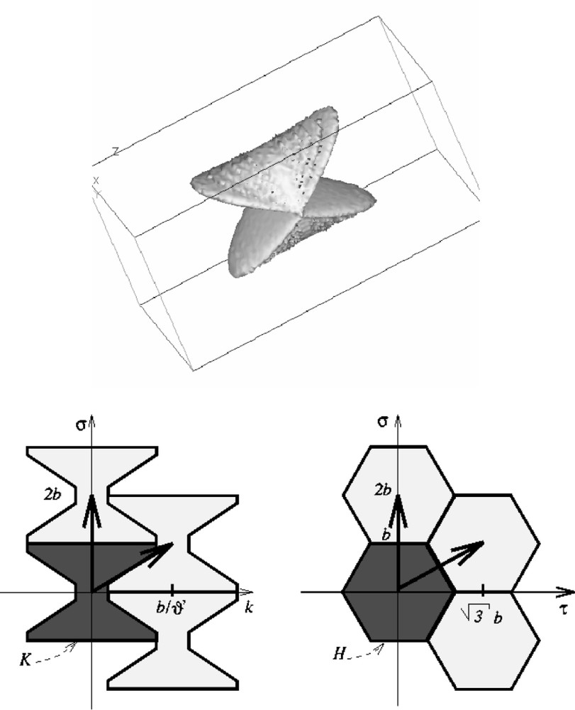
Top: 3D visualization of $𝐊_{3}$ from a random direction: outside this iso surface, ${\hat{g}}_{k} (σ, τ)$ is negligible. Bottom: non-overlapping sets $𝐊_{3} + 2 π W_{IH}^{- t} l, l \in ℤ^{3} :$ $𝐊_{3}$ is contained in the intersection of two perpendicular cylinders of respective base $𝐊$ and the hexagon H.

The minimal standard 3D orthogonal grid satisfying the non-overlapping conditions of the sets $𝐊_{3} + 2 π W^{- 1^{t}} l, l \in ℤ^{3}$ is generated by the matrix W_S, see (4). The interlaced scheme $W_{I} l, l \in ℤ^{3}$ satisfies also the non-overlapping condition of the sets $𝐊_{3} + 2 π {(W^{- 1})}^{t} l, l \in ℤ^{3},$ with twice less data than the best standard grid, see 〚16〛 $(\det W_{I} = 2 ϑ^{'} / ϑ \det W_{S}) .$

W_{S} = W_{S, ϑ} = \frac{π}{b} [\begin{matrix} ϑ & 0 & 0 \\ 0 & 1 & 0 \\ 0 & 0 & 1 \end{matrix}] W_{I} = \frac{π}{b} [\begin{matrix} 2 ϑ^{'} & - ϑ^{'} & 0 \\ 0 & 1 & 0 \\ 0 & 0 & 1 \end{matrix}]

4

with

ϑ^{'} = ϑ / (2 - ϑ) < ϑ < 1

(ϑ controls the exponential speed of convergence to zero of

\sum_{k} \int_{(k, σ, τ) \notin 𝐊_{3}} ∣ {\hat{g}}_{k} (σ, τ) ∣ d ξ

. It can be chosen close to 1 such that

b / ϑ \in ℕ

and

b / ϑ^{'} \in ℕ

). The interlaced scheme can be generated by an orthogonal detector grid of sampling steps

\frac{2 π}{b}

along the s-direction and

\frac{π}{b}

along the t-direction. The interlaced hexagonal scheme generated by the matrix

W_{IH} = \frac{π}{b} [\begin{matrix} 2 ϑ^{'} & - ϑ^{'} & 0 \\ 0 & 1 & 0 \\ 0 & - 1 / \sqrt{3} & 2 / \sqrt{3} \end{matrix}]

satisfies the sampling conditions (under weak assumptions: ϑ close to 1 and b sufficiently large, see 〚15〛). This scheme is

\frac{4 ϑ^{'}}{\sqrt{3} ϑ}

more efficient than the best 3D rectangular grid (and thus is more efficient than the interlaced one).

3 3D virtually invisible marker geometry

The main idea of our work is to make use of the redundancy of standard grids. Opaque markers are introduced in 3D (set of 2D projections) on such a way that, theoretically, the measured data are sufficient to interpolate the data which are not available because of the markers. We first remark that:

W_{S, ϑ^{'}} ℤ^{3} = W_{I} ℤ^{3} + (\frac{π}{b} {(ϑ^{'}, 1, 0)}^{t} + W_{I} ℤ^{3})

As 0<ϑ^′<ϑ<1, the matrix $W_{S, ϑ^{'}}$ satisfies the non-overlapping conditions of the set $𝐊_{3} + 2 π W_{S, ϑ^{'}}^{- t} ℤ^{3} .$ In practice ϑ is chosen close to 1, thus almost the same efficiency is obtained by $W_{S, ϑ^{'}}$ as by $W_{S, ϑ}$ because $\frac{ϑ^{'}}{ϑ}$ is then close to 1. Thus, if half of the standard points $W_{S, ϑ^{'}} ℝ^{3},$ located in the translated scheme $\frac{π}{b} {(ϑ^{'}, 1, 0)}^{t} + W_{I} ℤ^{3},$ are covered by opaque markers, then the half remaining scheme $W_{I} ℤ^{3}$ is enough to recover the full information. The same remark could be done with an hexagonal grid associated with the scheme 〚5〛. This idea is illustrated in Fig. 2 for an interlaced scheme. We solve the problem by reconstructing from the interlaced data. We then compute the full projections from the solution in order to show that the lacking data (supposed to be covered by markers) are well interpolated from the available interlaced data.

Fig. 2
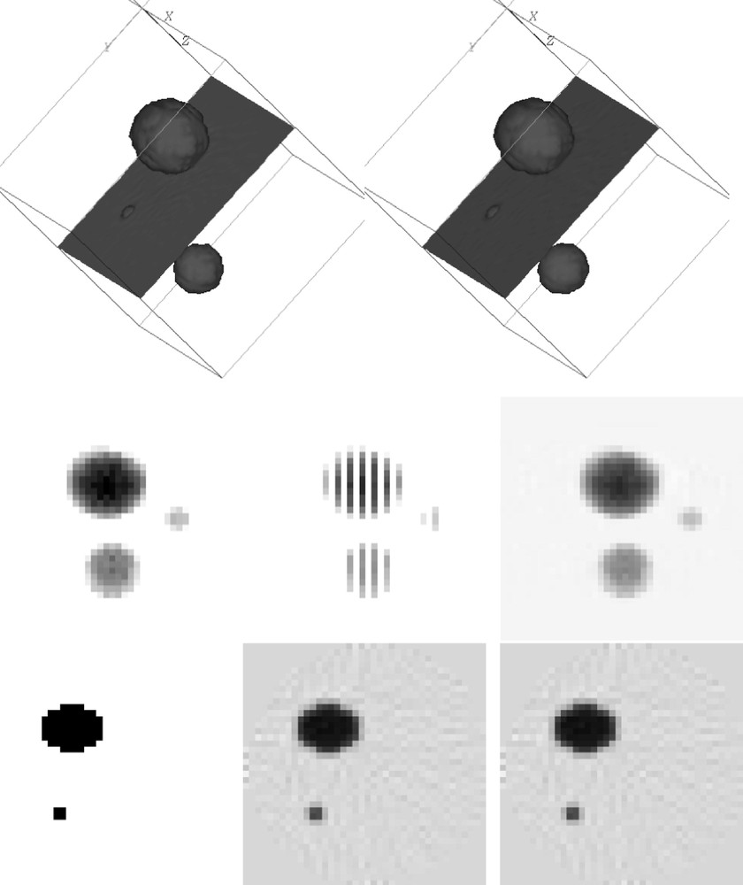
Top left: phantom to be reconstructed in a unitary cylinder. Top right: reconstruction from 63 interlaced parallel projections $(40 \times 40)$ on $[0, π] .$ Middle left: a standard projection from the original phantom. Middle centre: the corresponding interlaced projection; the vertical white lines do not receive any signal: they could be covered by markers. Middle right: projection of the reconstruction from the interlaced projection. Bottom left: slice of the phantom (position given in both top figures. Bottom center: corresponding slice in the reconstruction from the standard data. Bottom right: corresponding slice in the reconstruction from the interlaced data. As it can be seen from the last slices, the reconstruction from the interlaced data is not affected by particular artefacts as compared to the reconstruction from the complete standard data. The reconstruction from interlaced data is essentially the same as the reconstruction from standard data, even if half of the data is lacking. This confirms that no information is lost.

In practice, the calibration grids are sparse. However, in order to ensure that no information is lost, we interlace the calibration markers between two projections according to the results of previous section. The even projection are first measured. Afterwards we shift the calibration grid of one sampling unit (here the size of the ball) in the direction s. Then the odd projections can be processed. A simple algebraic approach is performed for the reconstruction from these data. We use a conjugate gradient on the regularized least squares problems

\min ∥ 𝐀 𝐟 - 𝐠 ∥^{2} + λ 𝐟^{𝑡} Δ 𝐟,

where

𝐀

is an ART-like matrix, f is a discretization of f in voxels, g is the vector of data, Δ is the positive Laplacian and

λ (> 0)

is a regularisation parameter automatically chosen by Generalised Cross Validation 〚17, 18〛. Because of the calibration grid, the geometry is irregular. The algorithm of this algebraic reconstruction essentially does not depend on the acquisition geometry: this is a major advantage for non-regular sampling.

In Figs. 3 and 4 we show reconstructions from both simulated and real data. In both cases, the X-ray source trajectory is half a circle around the measured object. Measurement geometry with image intensifiers are actually divergent. The distance of the source to the axis of rotation is approximatively seven times the diameter of the cylinder of reconstruction, thus the geometry is in fact almost parallel. In order to avoid a fast oscillating calibration marker grid, we can first acquire the even projection angles, then we can shift the calibration marker grid only once and finally we can acquire the odd projection angles.

Fig. 3
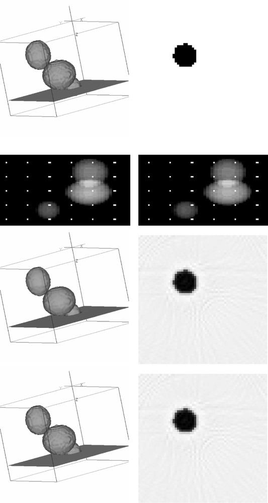
Top left: phantom to be reconstructed. Top right: slice in the phantom. Second line left: even projection with calibration markers. Second line right: odd projection with shifted calibration markers. Third line left: reconstruction from 90 projections with interlaced markers (60 × 50) on $[0, π] .$ Third line right: corresponding cross section. Bottom left: reconstruction from 90 projections without calibration markers. Bottom right: corresponding cross section. The reconstructions from projections with or without markers have the same quality.

Fig. 4
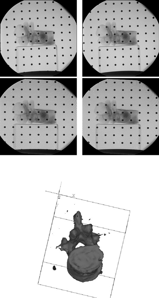
Top left: even projection with calibration markers. Top right: odd projection with shifted calibration markers. Second line left and right: after distortion correction. Third line: reconstruction from 60 projections $(113 \times 61)$ on $[0, π]$ with interlaced markers.

4 Interpolation on a standard scheme from interlaced data

Reconstruction from an irregular grid, such as in the presence of opaque markers, can also be achieved by interpolating the data on the complete standard grid and then using standard algorithms, as proposed in 〚19〛. In the following, we consider the Fourier interpolation on a standard scheme from an interlaced scheme in 2D tomography. This could be easily generalized to the 3D X-ray transform.

Let us suppose that half of the complete standard data are covered by markers. The geometry of the marker positions in the sinogram has to be interlaced such that the complementary interlaced data are still available. In this case, no information is lacking from the Shannon theory point of view. We propose here a Fast Fourier interpolation on a complete scheme from the data on an interlaced scheme.

In the general setting, the interlaced matrix W_I corresponding to a standard scheme

W_{S} = [\begin{matrix} h_{1} & 0 \\ 0 & h_{2} \end{matrix}]

is given by

W_{I} = [\begin{matrix} 2 h_{1} & - h_{1} \\ 0 & h_{2} \end{matrix}]

where h₁>0 and h₂>0 are the sampling steps of the standard scheme. We suppose that the essential support

𝐊

of the Fourier transform of the fonction

g (ϕ, s)

to be sampled satisfies the non-overlapping condition for both the standard and the interlaced scheme generated respectively by W_S and W_I with the same pairs of sampling steps

(h_{1}, h_{2}) .

From the Poisson formula associated to the interlaced scheme, we have:

\hat{g} (ξ) = {(2 π)}^{- 1} ∣ \det (W_{I}) ∣ . \sum_{k \in ℤ^{2}} g (W_{I} k) e^{- i ξ . W_{I} k} χ_{𝐊} (ξ)

8

In order to use the Fast Fourier Transform, we want to compute $\hat{g} (ξ_{l})$ according to (8) with:

ξ_{l} = 2 π N^{- 1} W_{S}^{- 1} l, l \in ℤ^{2}

9

where

N = diag (n_{1}, n_{2})

is the diagonal matrix containing the number of sampling points in each direction in the standard grid.

With the previous notations, we have:

\hat{g} (ξ_{l}) = {(2 π)}^{- 1} |\det (W_{I})| χ_{𝐊} (ξ_{l}) . (\sum_{m \in ℤ^{2}} g (W_{I} [\begin{matrix} 1 & 1 \\ 0 & 2 \end{matrix}] m) e^{- 2 i π (\frac{𝑙_{1} 𝑚_{1}}{𝑛_{1} / 2} + \frac{𝑙_{2} 𝑚_{2}}{𝑛_{2} / 2})} + \sum_{m \in ℤ^{2}} g (W_{I} [\begin{matrix} 1 & 1 \\ 0 & 2 \end{matrix}] m + W_{I} [\begin{matrix} 0 \\ 1 \end{matrix}]) . e^{- 2 i π (\frac{𝑙_{1} 𝑚_{1}}{𝑛_{1} / 2} + \frac{𝑙_{2} 𝑚_{2}}{𝑛_{2} / 2})} e^{- 2 i π (\frac{𝑙_{2}}{𝑛_{2} / 2} - \frac{𝑙_{1}}{𝑛_{1} / 2})})

Proof. The group $W_{I} ℤ^{2}$ is a subgroup of $W_{S} ℤ^{2} :$

W_{I} = W_{S} [\begin{matrix} 2 & - 1 \\ 0 & 0 \end{matrix}]

thus the group

W_{S}^{- t} ℤ^{2}

is a subgroup of

W_{I}^{- t} ℤ^{2} :

W_{I}^{- t} [\begin{matrix} 2 & 0 \\ - 1 & 1 \end{matrix}] = W_{S}^{- t}

10

thus from (9) and (10), we have:

e^{- i ξ_{𝑙} . 𝑊_{𝐼} 𝑘} = e^{- 2 i π 𝑁^{- 1} 𝑊_{𝑆}^{- 1} 𝑙 . 𝑊_{𝑆} [\begin{matrix} 2 & - 1 \\ 0 & 1 \end{matrix}] 𝑘}

or equivalently

e^{- i ξ_{𝑙} . 𝑊_{𝐼} 𝑘} = e^{- 2 i π 𝑁^{- 1} 𝑙 . [\begin{matrix} 2 & - 1 \\ 0 & 1 \end{matrix}] 𝑘}

We now remark that:

ℤ^{2} = \cup_{k \in ℤ^{2}} (k_{1}, 2 k_{2}) ⋃ \cup_{k \in ℤ^{2}} (k_{1}, 2 k_{2} + 1)

thus

[\begin{matrix} 2 & - 1 \\ 0 & 1 \end{matrix}] ℤ^{2} = 2 [\begin{matrix} 1 & - 1 \\ 0 & 1 \end{matrix}] ℤ^{2} \cup 2 [\begin{matrix} 1 & - 1 \\ 0 & 1 \end{matrix}] ℤ^{2} + {(- 1, 1)}^{t}

Using now

[\begin{matrix} 1 & - 1 \\ 0 & 1 \end{matrix}] ℤ^{2} = ℤ^{2}

or equivalently the bijective change of variable

[\begin{matrix} 1 & - 1 \\ 0 & 1 \end{matrix}] k = m \Leftrightarrow [\begin{matrix} 1 & 1 \\ 0 & 1 \end{matrix}] m = k

we can rewrite (8) as

\hat{g} (ξ_{l}) = {(2 π)}^{- 1} |\det (W_{I})| χ_{𝐊} (ξ_{l}) . (\sum_{m \in ℤ^{2}} g (W_{I} [\begin{matrix} 1 & 1 \\ 0 & 2 \end{matrix}] m) e^{- 2 i π (\frac{𝑙_{1} 𝑚_{1}}{𝑛_{1} / 2} + \frac{𝑙_{2} 𝑚_{2}}{𝑛_{2} / 2})} + \sum_{m \in ℤ^{2}} g (W_{I} [\begin{matrix} 1 & 1 \\ 0 & 2 \end{matrix}] m + W_{I} [\begin{matrix} 0 \\ 1 \end{matrix}]) . e^{- 2 i π (\frac{𝑙_{1} 𝑚_{1}}{𝑛_{1} / 2} + \frac{𝑙_{2} 𝑚_{2}}{𝑛_{2} / 2})} e^{- 2 i π (\frac{𝑙_{2}}{𝑛_{2} / 2} - \frac{𝑙_{1}}{𝑛_{1} / 2})})

Thus $\hat{g} (ξ_{l})$ can be computed from two FFTs of dimension $(n_{1} / 2, n_{2} / 2),$ based on the grid points $2 W_{S} ℤ^{2}$ and $2 W_{S} ℤ^{2} + W_{S} {(- 1, 1)}^{t}$ respectively. Indeed we have

W_{I} {(m_{1} + m_{2}, 2 m_{2})}^{t} = 2 W_{S} {(m_{1}, m_{2})}^{t}

and

W_{I} {(0, 1)}^{t} = W_{S} {(- 1, 1)}^{t}

The value of $g (W_{S} k)$ are then obtained by inverse FFT of the 2D grids points $\hat{g} (ξ_{l}) .$

In 2D tomography we can use $h_{1} = \frac{π}{p}$ where p is the number of projections on $[sqbl 0] 0, π [parr 0]$ and h₂=2/q (the reconstruction radius is normalised to 1). The sampling condition is that p must be slightly larger than $(π / 2) q$ (the band limit of f), see 〚14〛. In Fig. 5 we show a numerical example of the Fourier interpolation based on the previous development. This could be easily generalised to 3D problems.

Fig. 5
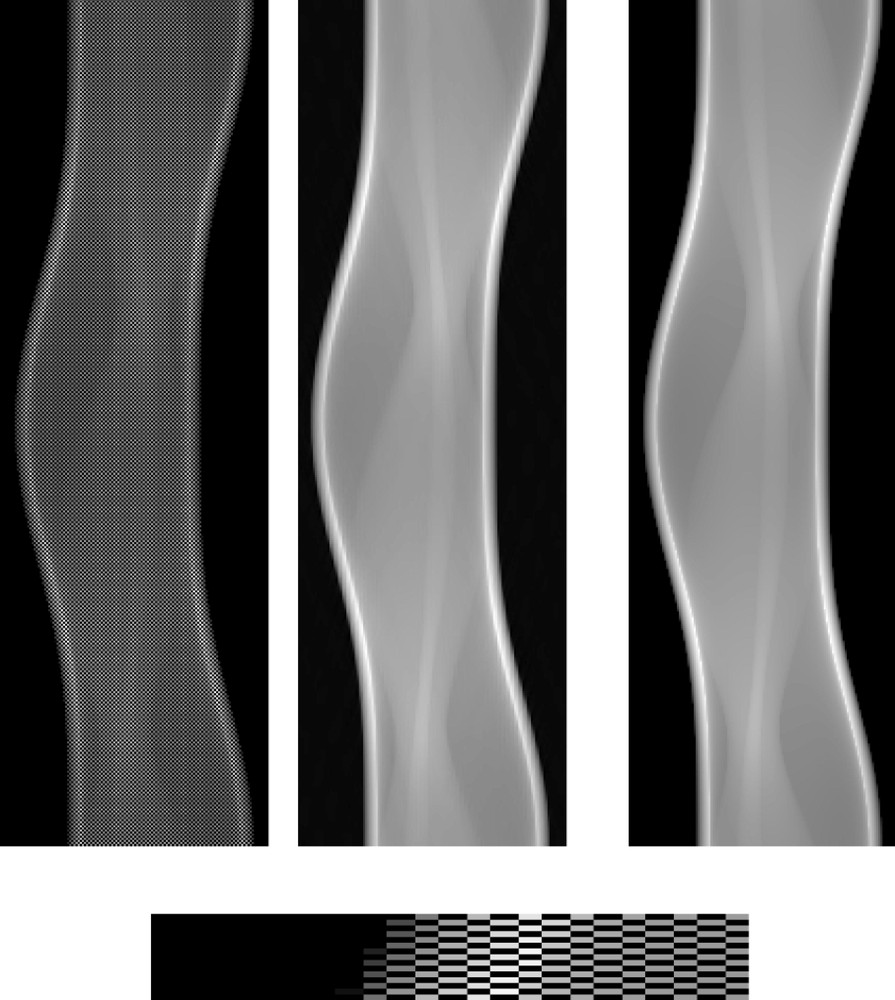
Top left: interlaced markers in a sinogram (p = 202 projections on $[sqbl 0] 0, π [parr 0]$ of q = 128 samples). Top centre: Fourier interpolation of the interlaced sinogram. Top right: corresponding standard sinogram. Bottom: zoom of a part of top left. We can see that the Fourier interpolation yields a very good interpolation of the lacking data (because of the markers).

5 Conclusion

In this work we have proposed interlaced geometries of markers for the dynamic calibration of image intensifiers. The design of these geometries is based on spectral properties of the 3D X-ray transform. For 2D or 3D reconstruction, these interlaced geometries of markers in the projections have almost no effect on the reconstruction. From the Shannon theoretical point of view, essentially no information is lost. We have illustrated this result with 3D reconstructions from both simulated and real data. We have given a Fast Fourier Transform based method for the interpolation on standard scheme from interlaced scheme in 2D. This interpolation scheme can be easily generalized to 3D. Interpolating on standards schemes from the available data first, allows then to use classical algorithms for the reconstruction.

Acknowledgements

We would like to thank Dr. Pierre Bessou from the neuroradiology department of the Grenoble University Hospital for providing the real data. This work have been supported by a grant of the Région Rhône-Alpes within the project “Santé et HP: de la Vision au Pilotage” and the project “ADéMo”.

Version abrégée

L'objectif de ce travail est de proposer de nouveaux schémas de grille de calibrage pour les amplificateurs de brillance dans le cadre de leur utilisation pour la reconstruction 3D en imagerie interventionnelle. Depuis plus de dix ans, la chirurgie assistée par ordinateur a connu de nombreux succès et a permis d'améliorer la précision de certains gestes pointus, tels que le vissage pédiculaire dans la chirurgie de la vertèbre. Ces progrès sont en partie dus à l'utilisation quantitative des images médicales lors des interventions chirurgicales. Les amplificateurs de brillance fournissent des images radiologiques en salle d'opération. Les distorsions dues au champ magnétique doivent être mesurées et corrigées. La technique habituelle de correction de ces distorsions est basée sur l'utilisation de mires de calibrage constituées d'une grille de marqueurs radio-opaques, qui permet d'estimer la distorsion (par la déformation de la grille), puis de corriger l'image. Dans le contexte de la reconstruction 3D, un grand nombre de projections radiographiques est transformé par un algorithme de reconstruction en une image 3D des coefficients d'atténuation de la région radiographiée. Nous nous sommes fixé l'objectif de construire une mire de calibrage furtive, dans le sens où cette mire serait visible dans chacune des projections et permettrait de corriger la distorsion dynamiquement sur chaque projection radiographique, mais ne supprimerait essentiellement pas d'information au sens de Shannon dans l'ensemble des projections. Comme nous le verrons, cet objectif peut être atteint par l'analyse des conditions d'échantillonnage du modèle de la mesure.

Après une correction de gain et d'offset, suivie d'une transformation logarithmique des données (selon la loi de Lambert–Beer, l'atténuation est exponentielle), le modèle utilisé pour la reconstruction en tomographie 3D est celui de la transformée en rayons X. Dans notre travail, nous limitons l'exposé à la géométrie parallèle, mais la démarche pourrait être généralisée aux géométries coniques, au moins numériquement. Dans le cas de la géométrie parallèle, si nous restreignons la trajectoire de la source et du détecteur à un cercle, nous pouvons mesurer la fonction d'atténuation $f \in C_{0}^{\infty} (Ω)$ à reconstruire par :

g (ϕ, s, t) = \underset{- \infty}{\int^{+ \infty}} f (s θ + t e_{3} + u ζ) d u

où ζ∈S¹ est le cercle unité,

Ω

est le cylindre unité de

ℝ^{3},

ϕ \in [0, 2 π [

,

ζ = {(- \sin ϕ, \cos ϕ, 0)}^{t},

θ = {(\cos ϕ, \sin ϕ, 0)}^{t},

e_{3} = {(0, 0, 1)}^{t},

s \in [- 1, 1],

t \in [- 1, 1]

et

(s, t)

sont les coordonnées du pixel de mesure sur le détecteur (plan) de radiographie.

Dans un premier temps, nous rappelons les conditions d'échantillonnage de g lorsque f est supposée essentiellement b-bande limitée $(b > 0) .$ Elles sont basées sur l'identification du support essentiel de la transformée de Fourier de g. On peut montrer que les schémas standards (équidistants en φ, s et t), c'est-à-dire les grilles rectangulaires dans l'espace des paramètres, sont redondants. Le meilleur schéma standard (ensemble des points $W_{S} k, k \in ℤ^{3}$ ) est presque deux fois moins performant que le schéma entrelacé (ensemble des points $W_{I} k, k \in ℤ^{3}$ ) avec:

W_{S} = W_{S, ϑ} = \frac{π}{b} [\begin{matrix} ϑ & 0 & 0 \\ 0 & 1 & 0 \\ 0 & 0 & 1 \end{matrix}]; W_{I} = \frac{π}{b} [\begin{matrix} 2 ϑ^{'} & - ϑ^{'} & 0 \\ 0 & 1 & 0 \\ 0 & 0 & 1 \end{matrix}]

où

ϑ^{'} = ϑ / (2 - ϑ) < ϑ < 1 .

On peut remarquer que :

W_{S, ϑ^{'}} ℤ^{3} = W_{I} ℤ^{3} + (\frac{π}{b} {(ϑ^{'}, 1, 0)}^{t} + W_{I} ℤ^{3})

où

\frac{ϑ^{'}}{ϑ}

est proche de 1 si ϑ est proche de 1. Donc, si nous choisissons

W_{S, ϑ^{'}} ℤ^{3}

comme schéma d'échantillonnage de g (schéma standard quasi optimal, si

\frac{ϑ^{'}}{ϑ}

est proche de 1), alors si des points recouverts de marqueurs opaques sont seulement choisis dans le schéma

(\frac{π}{b} {(ϑ^{'}, 1, 0)}^{t} + W_{I} ℤ^{3}),

alors

W_{I} ℤ^{3}

restera intact. Comme le schéma

W_{I} ℤ^{3}

satisfait les conditions de Shannon sur g, il permet d'interpoler quasi exactement g sur tout son domaine, donc y compris sur les points de mesure remplacés par des marqueurs de calibrage. Cette idée conduit à la réalisation d'une mire de calibrage rectangulaire de pas

2 q \frac{π}{b} ϑ^{'}

dans la direction θ et

p \frac{π}{b}

dans la direction e₃, avec p et q deux entiers naturels strictement positifs. En pratique

\frac{π}{b} ϑ^{'}

sera un multiple entier du nombre de pas d'échantillonnage sur le détecteur réel. Cette mire doit être translatée de

\frac{π}{b} ϑ^{'} θ

pour les projections impaires. Ainsi, les marqueurs de calibrage se trouvent toujours dans un schéma entrelacé.

Après quelques expérimentations numériques, nous proposons dans la dernière partie une méthode d'interpolation de Fourier rapide d'un schéma entrelacé vers un schéma standard. Ceci permet de montrer numériquement un exemple simulé en tomographie 2D que la suppression d'une moitié des points d'échantillonnage (supposés recouverts de marqueurs de calibrage) n'enlève essentiellement pas d'information au sens de Shannon et que cette information peut-être retrouvée efficacement par des techniques de transformée de Fourier rapide.

Bibliographie

[〚1〛] I.A. Feldkamp; L.C. Davis; J.W. Kress Practical cone-beam algorithm, J. Opt. Soc. Am. A, Volume 1 (1984), pp. 612-619

[〚2〛] P. Grangeat Reconstruction d'images tridimensionnelles, thèse d'habilitation à diriger des recherches, INPG, 1993

[〚3〛] M. Defrise; R. Clack Cone-beam reconstruction using shift variant filtering and cone beam backprojection, IEEE Trans. MI, Volume 13 (1994), pp. 186-195

[〚4〛] H.K. Tuy An inversion formula for cone-beam reconstruction, SIAM J. Appl. Math., Volume 43 (1983), pp. 546-552

[〚5〛] A.K. Louis; P. Maass Contour Reconstruction in 3-D X-Ray CT, IEEE Trans. Med. Imaging, Volume 12 (1993), pp. 764-769

[〚6〛] M. Defrise; R. Clack; D. Townsend The solution to the 3D image reconstruction problem from 2D parallel projections, J. Opt. Soc. Am. A, Volume 10 (1993), pp. 869-877

[〚7〛] M. Defrise A factorizatiom method for the 3D X-ray transform, Inverse Problems, Volume 11 (1995), pp. 983-994

[〚8〛] S. Schreiner et al. A system for percutaneous delivery of treatment with a fluoroscopically-guided robot, CVRMed-MTCAS'97, LNCS 1205, Springer, 1997, pp. 747-756

[〚9〛] J. Chabbal et al. Amorphous silicon X-ray image sensor, Proc. SPIE 2708, 1996, pp. 499-510

[〚10〛] G. Champleboux; S. Lavallee; P. Sautot; P. Cinquin Accurate calibration of cameras and range imaging sensors, the NPBS method, IEEE Int. Conf. on Robotics and Automation, Nice France, May 1992 , pp. 1552-1558

[〚11〛] A.M. Cormack Sampling the Radon transform with beams of finite width, Phys. Med. Biol., Volume 23 (1978), pp. 1141-1148

[〚12〛] P.A. Ratteyand; A.G. Lindgren Sampling the 2-D radon transform, IEEE Trans. ASSP, Volume 29 (1981), pp. 994-1002

[〚13〛] D.P. Petersen; D. Middleton Sampling and reconstruction of wave-number-limited functions in n-dimensional Euclidean space, Inf. Control, Volume 5 (1962), pp. 279-323

[〚14〛] F. Natterer The Mathematics of Computerized Tomography, Wiley, 1986

[〚15〛] L. Desbat Echantillonnage parallèle efficace en tomographie 3D, C.R. Acad. Sci. Paris, Série I, Volume 324 (1997), pp. 1193-1199

[〚16〛] L. Desbat Efficient sampling in 3D tomography: parallel schemes (P. Grangeat; J.-L. Amans, eds.), Three-Dimensional Image Reconstruction in Radiology and Nuclear Medicine, Kluwer Academic, 1996, pp. 87-100

[〚17〛] D.A. Girard A fast Monte Carlo cross-validation procedure for large least squares problems with noisy data, Numer. Math., Volume 56 (1989), pp. 1-23

[〚18〛] D.A. Girard Asymptotic optimality of the fast randomized versions of GCV and C_L in ridge regression and regularisation, Ann. Stat., Volume 19 (1991), pp. 1950-1963

[〚19〛] A. Faridani An application of a multidimensional sampling theorem to computed tomography, AMS-IMS-SIAM Conference on Integral Geometry and Tomography, Contemporary Mathematics, volume 113, 1990, pp. 65-80

Commentaires - Politique