

Version française abrégée
Les forêts naturelles sont caractérisées par un haut niveau d'hétérogénéité à la fois spatiale et temporelle. Cette hétérogénéité se retrouve dans tous les domaines (composition de la végétation, âge des arbres, statut nutritionnel, etc.). Les patrons de végétation observés à un moment donné résultent de la superposition des contraintes liées aux gradients environnementaux, des effets des perturbations dans le temps et dans l'espace et de la biologie des espèces. L'échelle de la structuration observée dépend des échelles de variabilité des habitats et des perturbations. Des événements climatiques extrêmes, comme les tempêtes ou les grands coups de gel, induisent une structuration à grande échelle, les attaques d'insectes ou les incendies induisent plutôt une structuration de grande à moyenne échelle, alors que la chute d'un vieil arbre, par exemple, va induire une structuration à petite échelle. Ces différentes influences structurent la forêt en une mosaı̈que de populations et d'habitats organisés à plusieurs échelles spatiales. Certaines études montrent tout de même que les processus les plus importants dans la création et la maintenance de l'hétérogénéité des forêts en climat tempéré sont les perturbations de la canopée de petite taille. Ces perturbations locales libèrent à la fois de la place pour la régénération, de la lumière et des nutriments.
L'analyse de la réponse de la croissance radiale des arbres permet d'évaluer l'impact de ces perturbations sur la croissance du peuplement et de reconstruire leurs occurrences dans le temps. L'originalité de ce travail est d'associer des techniques utilisées en dendrochronologie pour détecter les perturbations avec une analyse spatiale fine de la structure du peuplement (âge, diamètre, hauteur) et des perturbations elles-mêmes. Deux processus sont étudiés dans ce travail : la colonisation et les perturbations, suivant chaque fois l'hypothèse que la structure spatiale est un attribut du fonctionnement de l'écosystème.
Cette étude a été réalisée dans un peuplement de pins à crochets, en limite supérieure de la forêt. Le lieu-dit se nomme Clôt Enjaime (latitude N44°56′17 ; longitude E6°42′20 ; altitude 2200 m), il est situé sur la commune de Montgenèvre, près de Briançon dans les Alpes internes du Sud. L'ensemble du site d'étude recouvre une superficie de 1 ha à peu près. À l'intérieur de ce site, deux placettes ont été délimitées, dans lesquelles la structure du peuplement est plus finement analysée. Ces deux placettes sont désignées par les termes de clôt1 (située à l'intérieur de la forêt) et clôt2 (située en limite supérieure de la forêt).
Deux stratégies d'échantillonnage ont été menées en parallèle au cours de cette étude. À l'échelle du site, 45 arbres ont été carottés, dans le but de construire une chronologie maı̂tresse. En ce qui concerne les placettes, tous les arbres (soit 91 arbres supplémentaires) ont été carottés (afin d'obtenir leurs âges) et mesurés (en hauteur et en diamètre). Afin de permettre l'analyse de l'organisation spatiale du peuplement et des séquences de perturbation, chaque arbre a été positionné spatialement à l'aide d'une photographie aérienne et d'un modèle numérique de terrain, tous deux géoréférencés.
L'histoire des perturbations ayant affecté un site peut être reconstruite à l'aide de chronologies d'épaisseur de cernes par le calcul d'un indice adapté : %GC. Cet indice est la différence entre deux moyennes mobiles calculées sur deux fenêtres de 10 ans consécutives. Il marque l'occurrence d'une perturbation sans décalage temporel. Habituellement, pour une forêt fermée, on considère qu'il y a eu perturbation quand le %GC passe au-dessus de 25 %. Dans le cadre de ce travail (pour les forêts subAlpines), un seuil de 10 % paraı̂t mieux convenir. Par ailleurs, l'analyse spatiale du %GC permet de s'affranchir de ce seuil arbitraire. Les quatre variables décrites précédemment (diamètre, hauteur, âge, et %GC) font ensuite l'objet d'une analyse spatiale. L'autocorrélation spatiale de ces variables est recherchée par le calcul de la semivariance et la réalisation d'un semivariogramme. Dans le cas du %GC des cartes ont également été produites par krigeage.
L'étude de la structure démographique des placettes met en évidence une organisation de la population en cohortes. Cette organisation se retrouve aussi pour le diamètre. Les âges et les diamètres sont plus élevés dans clôt1 que dans clôt2. Ceci met en évidence un processus de colonisation des pâturages par la forêt. De plus, l'organisation en cohorte de la population montre que cette colonisation se fait par avancées saltatoires de groupes pionniers.
La hauteur, quant à elle, décroı̂t progressivement avec l'altitude. Ceci met en évidence un fort gradient écologique de diminution de la production avec l'augmentation des contraintes climatiques liées à l'altitude. Remarquons que dans de tels peuplements subalpins, seul un échantillonnage très rigoureux et bien maı̂trisé peut permettre de s'affranchir de ce biais pour étudier le comportement du peuplement vis-à-vis du climat et des changements climatiques.
L'analyse spatiale du %GC n'a pu se faire que sur la perturbation de 1964, en raison de la diminution du nombre de données disponibles au fur et à mesure que l'on remonte dans le temps. L'étude de cette perturbation montre cependant clairement la cohérence des deux méthodes (spatiale et temporelle). L'augmentation du %GC n'est pas due à un phénomène diffus, mais bien à la réaction très forte d'un groupe d'arbres proches les uns des autres. De plus, la surface de la tache perturbée diminue en même temps que le %GC décroı̂t. Ceci permet de dire que la zone de réponse à la perturbation de 1964 est de petite taille (entre 0,035 et 0,073 ha) et que ses effets ont été ressentis par le peuplement pendant six ans.
L'analyse dendroécologique des régimes de perturbation est aujourd'hui un outil régulièrement employé et efficace. Nous montrons cependant dans ce travail que le couplage de ces techniques à une analyse spatiale permet, non seulement de s'affranchir de certaines formulations arbitraires, mais surtout de mieux comprendre la nature et le fonctionnement des perturbations, en complétant leur portrait temporel par leur portrait spatial.
1 Introduction
Natural forests are characterised by a high level of both spatial and temporal heterogeneity. This heterogeneity encompasses all the features of the forest structure (vegetation composition, age structure, physiological status, etc.). The observed vegetation patterns result from environmental gradients (soil, topography, and microclimate) and disturbances patterned in time. The spatial scale of the observed patterns depends on the scale of habitat variability and the scale of the disturbances. Climate events, like windstorms or frost, will induce broad scale patterns, and insect outbreaks or fires may induce broad to medium scale patterns, while singletree falls will result in small-scale patterns. As a result, forests are composed of a shifting mosaic of populations and habitats [1,2]. Some studies have shown that the major process involved in the creation and maintenance of forest heterogeneity in temperate climates is small-sized canopy disturbance [1,3]. These local disturbances release regeneration sites [4,5]. The openings also modify the growth conditions of the remaining trees, especially light and nutrient availability [6–9].
The analysis of growth responses in trees using a radial-growth averaging technique [3,10,11] allowed the detection of such growth responses and the reconstruction of the time sequence of the disturbances. Some workers associated dendrochronological studies in time with a spatial approach by mapping the cored trees [3,12,13]. Others used spatial analysis to study the patterns of tree sizes and age of forest vertical or horizontal diversity [14,15], but do not use dendrochronological data. Following the methodology of these previous works, we coupled the reconstruction of disturbance events in time with the spatial analysis of forest tree structure. Geostatistical techniques including semivariograms and krigeage allow analysis of both spatial structure of forest stands and spatial patterns of disturbances.
We focussed on two processes: colonisation and disturbance. The colonisation patterns were analysed through simple variables (tree height, diameter and age). For disturbance, we followed the postulate of Nowacki and Abrams [11], which is that the shape and the size of the disturbance will provide information as to the nature of the disturbance. We hypothesised that the spatial structure of this forest would be linked to the functioning of these two processes.
2 Materials and methods
2.1 Study site
The study site is located in the inner southern French Alps (Fig. 1), close to the city of Briançon, and close to the village of Montgenèvre, at a place called Clôt Enjaime (latitude N44°56′17; longitude E6°42′20; altitude 2200 m). The climate is continental, with Mediterranean influences in summer. The annual average precipitations for the meteorological station of Briançon (1340 m) during the last 30 years are 750 mm and the mean annual temperature is 7.8 °C (on average the temperature in the area decrease by 0.4–0.6 °C per 100 m of increasing elevation and precipitation increases by ca 10%). The site is located at the upper limit of a mountain pine (Pinus uncinata) forest. Under the studied site stands a subAlpine conifers forest (with Pinus uncinata and Pinus sylvestris) and above it stands an Alpine grass. The studied site extends over an area of 1 ha.
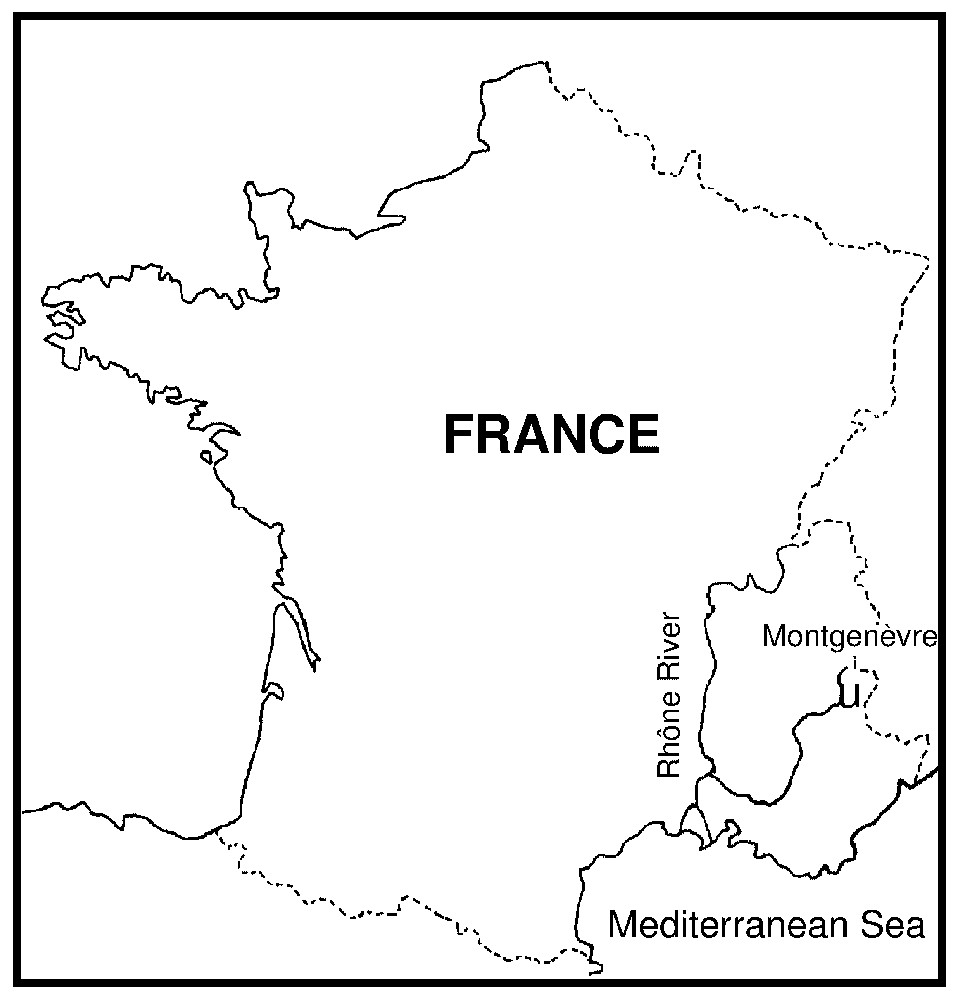
Location of the study area in the French Alps.
Forest stands in the area of Montgenèvre are no longer exploited since the World War II, because the wood had received too much lead shot. According to the indications of the local forester, we believe that the studied stand was not intensively managed before this period. Indeed mountain pine is not a widely used species and the location of the stand is not very accessible. So, we assume that the internal dynamic of the stand is the results of a natural process with few anthropogenic influences. On the other hand, we assume that the external dynamic of the stand is determined by anthropogenic activities with the progressive abandon of the pasture since the World War I.
2.2 Tree sampling and coring
Tree sampling and coring were completed in a two-steps approach combining two spatial levels: the site level and the plot level. The plots are constituted by two discs of about 150 m in diameter delineated into the site in order to analyse finely the forest structure. For the rest of the text, we will use the term ‘site’ to indicate the main site of Clôt Enjaime, and the term ‘plots’ for the two plots: clot1 (within the main forest) and clot2 (at the upper forest limit).
At the site level, trees are shared in three groups according to their diameters: small (D⩽20 cm); medium (20<D⩽40 cm) and large (D>40 cm). For each group, the 15 higher trees were cored at breast height. These 45 trees formed sample 1. For the large group, three cores were taken from each tree. The first one was taken uphill, the two others at 120 ° to the first one. For the small- and medium-diameter-class trees, we took only one core through the trunk, which is parallel to the elevation lines. This sampling procedure, because young trees are actually easier to cross-date than old ones, allows gaining times in the data collection and measure.
At the plot level, a systematic sampling was done. Inside the plots some trees belong to the sample 1 and have already been cored (45 trees). All the other trees, above 1.30 m, included within the plots are cored at the trunk base. These 91 news trees (42 for clot1 and 49 for clot2) form sample 2.
Diameter at breast height and total tree height were measured for all the trees belonging to samples 1 and 2. All the sampled trees were marked with a metallic numbered tag.
2.3 Tree mapping
A raw map of the sampled trees positions was drawn in the field using an enlarged copy of a 1:25 000 geographic map in order to help the location of trees on an aerial photograph. Using a GIS (IDRISI, Clarks Labs), we precisely mapped all the trees in the study site (both samples 1 and 2) using a panchromatic aerial photo taken in June 1996 by the French National Geographical Institute (IGN) (ref.: 7638, 1996, approximate scale: 1:12 500). The photo was scanned at a 50-cm resolution and orthorectified according to a local digital elevation model, computed from digitised elevation lines of 10 m and interpolated linearly to a resolution of 1 m.
Since the tree density is low, the individual canopy of each tree could be identified. A point located at the middle of the canopy was considered to be the actual position of the trunk. Since the local slope is moderate (25–30%), we considered that it has no effect on the congruence of relative positions of the geometric centres of the tree crowns and the tree trunk position on the ground. The tree trunk point map was used to obtain the tree coordinates used to compute the spatial statistics (Fig. 2).
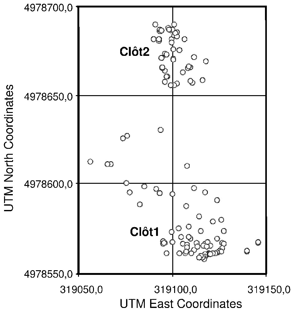
Trees location map computed from an orthorectified panchromatic aerial photograph. The UTM coordinates refer to the UTM zone N31.
2.4 Dendrochronological data
For sample 1, ring-width chronologies were constructed using classical techniques [16]. After the series were checked and cross-dated [17], raw elementary (for one core) chronologies were averaged to generate individual (for one tree) chronologies and one master chronology for the site.
For sample 2, the number of rings was counted to obtain an age estimate.
2.5 Dendrochronological analysis
If large-scale disturbances (extreme climatic events, severe insect outbreaks) are usually directly visible on the mean chronology, detection of medium- and small-scale disturbances needs more sophisticated methods of signal analysis.
According to Lorimer and Frelich [6], disturbance history can be derived from tree ring series. After a disturbance that eliminated one or several trees, nearby trees produce measurable growth increases. These patterns indicate competition releases. According to Nowacki and Abrams [11], a difference between two consecutive moving averages (the growth change index) with a 10-years window was computed. The moving average also allows the standardisation of individual dendrochronological series [6]. The growth change index is expressed as a percentage, according to the following formula:
| (1) |
The ten-year window allows us, first, to preserve the disturbance events that are usually associated with the medium-frequency signal, and second, to eliminate the high- and low-frequency signal (age, geometric and climatic effects) in the obtained index [11]. In order to verify this assertion, we have checked that the obtained %GC chronology is totally independent of climate on the one hand, and of trees ages on the other hand.
Some authors consider that a disturbance event has occurred when the %GC is higher than 25% [6,11,18,19]. We suggest, for subAlpine forest, a threshold of 10%; indeed, a higher threshold would have ignored small-scale disturbances at the stand level because of the low density of trees found here. Two other disturbance indicators are associated with the mean %GC. The first one is the number of trees with individual %GC above the 25% threshold. The second one is the demographic patterns present, i.e. the occurrence of cohorts. It is considered that the number of trees above the 25% GC threshold indicates the disturbance extent, while the number of trees installed after the disturbance indicates the disturbance intensity [11].
2.6 Spatial analysis
The 25% or 10% threshold of disturbance detection addresses the event signal at the stand level, but provides no clues on the event's shape and location. Those two characteristics could help interfering the perturbation cause. We ought to know if the %GC is spatially autocorrelated as autocorrelation patterns would give us additional insight into the disturbance event nature. A variable is said to be autocorrelated or regionalised if it is non-randomly patterned in space or in time. The autocorrelation structure could be described by using structure functions [20]. Semivariance is one of these measures [21]. The semivariance was designed by geologists, as a tool for estimating the quantity of minerals between samples. The total variance is distributed into local variances according to the distance between samples [22]. This method was proposed as a spatial analysis tool in ecology [23]. Semivariance can be plotted as a function of distance. The graph obtained is called a semivariogram. The formula is:
| (2) |
Several parameters can be estimated from the semivariogram. The range defines the distance beyond which there is no correlation between the samples. The sill is the level of semivariance at the range. The nugget effect refers to the occurrence of a variance for null distance. It means that an inherent variance exists, which could result from random variation or from a too coarse sampling scheme. If the semivariogram is a flat line, this means that there are no spatial patterns. In other cases, a spatial pattern exists. Functions can be fitted to the semivariogram, in order to determine the range and the sill and to interpolate data using the kriging method [22,24]. It is also possible to analyse the spatial patterns according to their directions in order to determine anisotropy levels. Nevertheless, while curve fitting allows an optimal interpolation, each theoretical function means a model of underlying spatial pattern that could also be interpreted without fitting.
We computed for each variable (age, diameter, height and %GC) a semivariogram and fitted a function. Maps were then derived by kriging using the geostatistical analysis programs: Surface III+ 2.6©″ from the Kansas Geological Survey (1995) and GS+ 5.1© Gamma Design Software (2001).
3 Results
3.1 Stand structure and colonisation patterns
We first studied the demographic structure of the Pinus uncinata population at the plot level. From age frequency distributions, a cohort pattern becomes evident (Fig. 3). For the clot1 stand, we observed three recruitment phases: one during the period 1950–1970, one during the period 1890–1900 and the last one during the period 1850–1860. The trees belonging to this three age cohorts are today respectively in the ranges 30–50, 100–110 and 140–150 years old. For the clot2 stand we observed 2 recruitment phases: the first during the period 1960–1970 and the second during the period 1920–1930. The trees belonging to this two age cohorts are respectively today between 30–40 and 70–80 years old. Seedling recruited after 1980 do not often reach 1.30 m today, so most of them have not been sampled. Consequently, our sampling strategy does not allow interpreting recruitment data after this date.
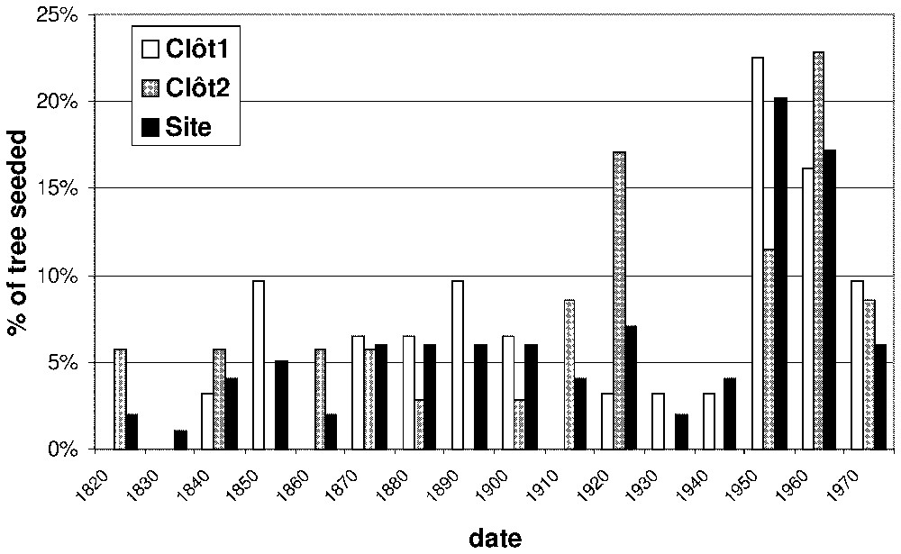
Age frequencies of the trees for the global site and the two plots (clôt1 and clôt2). The seeded year was estimated from the cambial age of the tree cores.
Similar patterns can be observed for diameter and height. The modal diameter classes are 20 and 40 cm at clot1 and 10 and 30 cm at clot2. The average diameter is 19.72 cm for clot1 and 13.46 cm for clot2. For height, the modal classes are 3 and 10 m for clot1 and 1, 3 and 6 m for clot2.
For age structure, the semivariogram allowed us to identify aggregated patterns. The range is 22 m for clot1 and 16 m for clot2 and 15.63 m at the site level (Fig. 4). We also found this pattern for diameter: the ranges are 14 m for clot1, 13 m for clot2 and 15.61 m for clôt Enjaime as a whole (Fig. 5). For height, we observed a linear gradient, suggesting an environmental gradient (Fig. 6).
Isotropic semivariogram of the Clôt Enjaı̂me tree ages fitted with a spherical model. Spherical model: C0=0.101; C0+C=0.385; A0=12.72; r2=0.912; RSS=3.065×10⁻³.
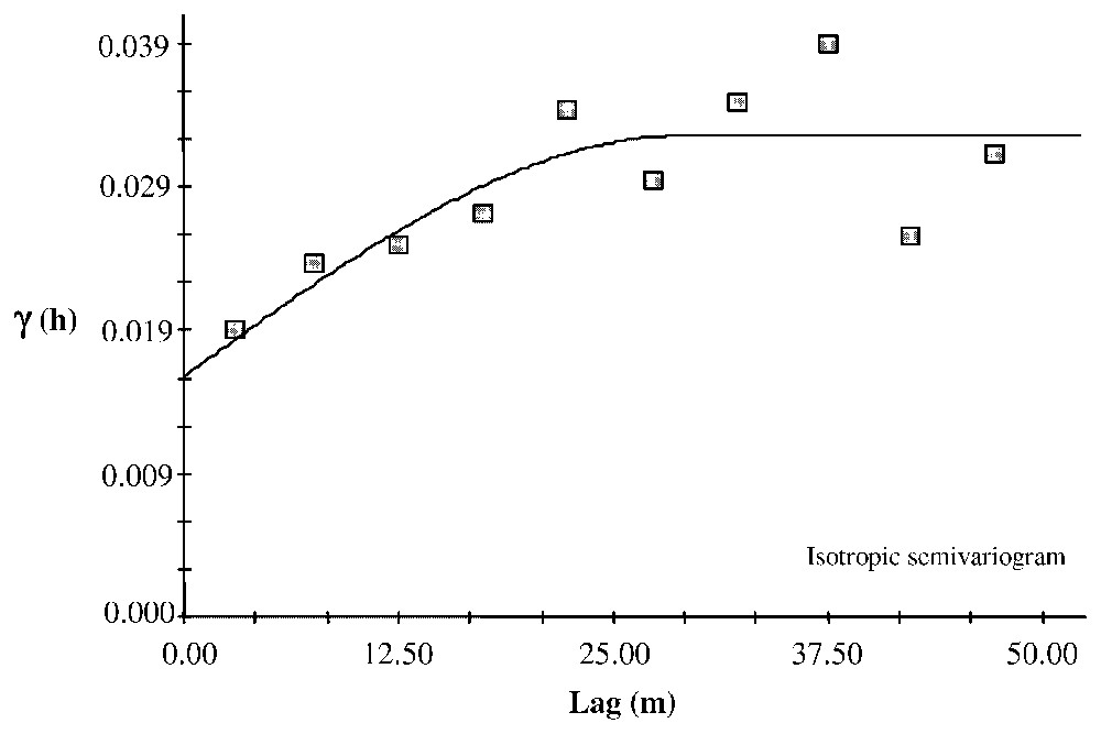
Isotropic semivariogram of the Clôt Enjaı̂me tree diameter fitted with a spherical model. Diameter was measured at breast height. Spherical model: C0=0.01625; C0+C=0.03260; A0=29.10; r2=0.628; RSS=1.160×10⁻⁴.
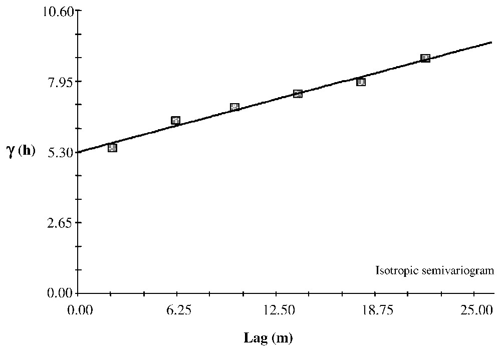
Isotropic semivariogram of the Clôt Enjaı̂me tree height fitted with a linear model. This model suggests a gradient pattern over the site. Linear model: C0=5.2972; C0+C=8.7469; A0=21.92; r2=0.980; RSS=8.30.
3.2 Disturbance event reconstruction
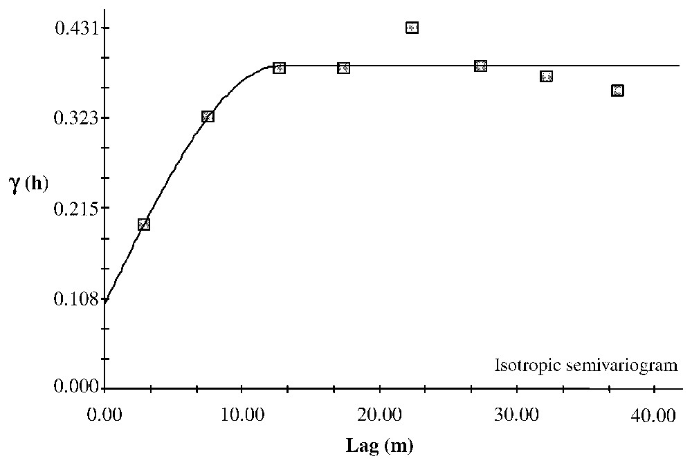
The mean chronology measured at Clôt Enjaime goes back to 1830 (Fig. 7a). Only one disturbance event exceeds the 25% threshold (Fig. 7b). However, four others exceed a 10% threshold. These events occurred in 1865, 1898, 1922, 1964 and 1988. Only the 1964 event allows analysis of the spatial patterns of the individual trees' %GC, because for the two older events the number of trees is too low for computing geostatistics (Fig. 7c) and the last one is too close to the end of the record to be analysed. The semivariogram computed from the 1964 %GC indicates an autocorrelation pattern and could be fitted using several structure functions with sill (Fig. 8). We fitted three models: spherical (r2=0.875), linear to sill (r2=0.912) and Gaussian (r2=0.902). The range, which could be interpreted as the mean distance of the spatial disturbance event response, varies from 33.6 m (linear to sill model) to 48.2 m (spherical model). The Gaussian model has a range of 42.4 m.
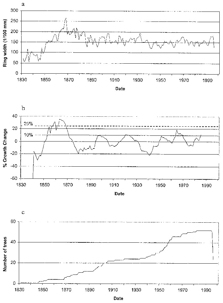
(a) Master chronology of Clôt Enjaı̂me; (b) chronology of %Growth Changes for the Clôt Enjaı̂me site; (c) number of trees available per year.
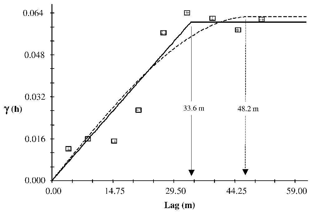
Isotropic semivariogram of the %Growth Change during the disturbance event of 1964. Two models have been fitted to the results: the plain line is a linear to sill model and the dotted line is a spherical model. The two arrows indicate the ranges given by both models. Linear to sill model: C0=0.00010; C0+C=0.06020; A0=33.60; r2=0.912; RSS=3.821×10⁻⁴. Spherical model: C0=0.00010; C0+C=0.06240; A0=48.20; r2=0.875; RSS=5.4021×10⁻⁴.
The ranges obtained could be used to estimate the area affected by the disturbance response and considering in first stance that the disturbance response is roughly circular (in that case, the area is π× range2). Finally, the disturbance area could be estimated to vary between 0.035 ha and 0.073 ha according to the structure model fitted.
A map of the 1964 %GC was derived by kriging (Fig. 9a). We can observe a patch of very high %GC that clearly identifies the location and the shape of the disturbance.
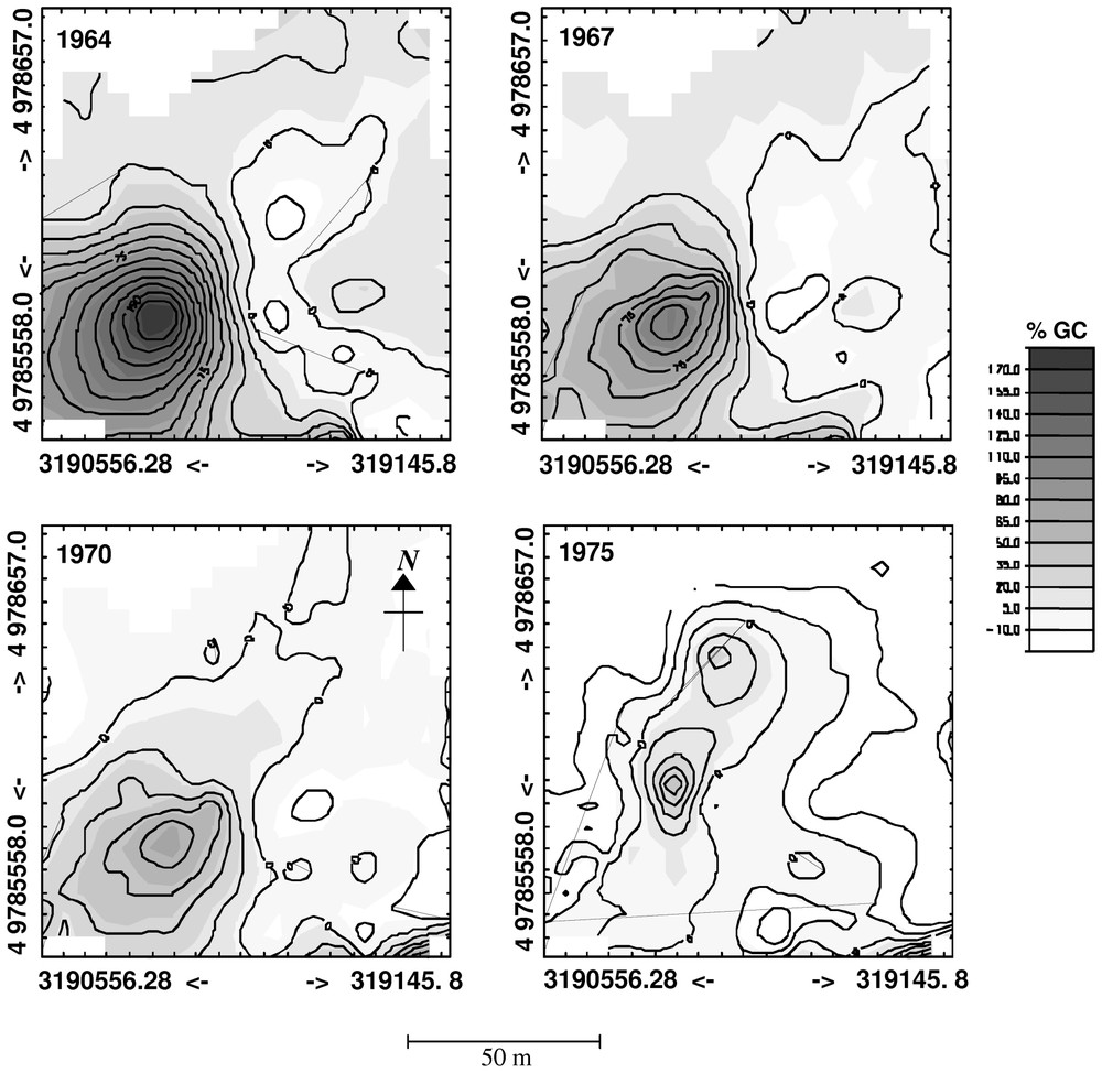
Kriged maps of %Growth Change (%GC) for 1964 (a), 1967 (b), 1970 (c), and 1975 (d). We can observe that the %GC fades out with time after disturbance from 1964 to 1975. The grey scale indicates the intensity of %GC from white (low %GC) to dark grey (high %GC). The spatial coordinates refer to the UTM zone 31N geodesic system.
We also computed the semivariogram and the krigged maps for the following years (1967, 1970, and 1975). We observed that with time the disturbance response fades out (Fig. 9) and that the semivariogram changed from a curve in 1964 to a flat line after 1970. This indicates that there was no longer a spatial pattern of %GC, and that tree growth became homogeneous at the stand level.
4 Discussion
The analysis of the demographic structure of the trees population coupled with spatial analysis makes clear the aggregated pattern of this Pinus uncinata forest located at the timber line. The age classes are organised in cohorts combined with spatial aggregates. Several authors who worked in subAlpine or boreal forests [13,25,26] described this kind of forest pattern. The upper stand (clot2) appeared to be younger than the lower stand (clot1), what is interpreted as an evidence of the re-colonisation dynamics of former altitude pastures, now abandoned. The former land use of this area is, documented by the location name ‘clôt’, which means ‘closed pasture’. We interpreted the aggregate pattern of recolonisation as a result of extreme environmental conditions at that altitude. Tree communities progress by seed establishment in favourable habitats or during favourable seasons. Once a tree or a group of trees developed, it becomes a new centre of dispersal. This kind of behaviour should become more and more important with increasing altitude and/or extreme environmental conditions. The new group of trees constitutes a shelter by creating a more favourable environment for the following cohorts of trees. This process is close to the nucleation model [27].
In a work on spatial pattern of a subAlpine forest-Alpine pasture ecotone Camarero and Gutierrez [28] found very similar results concerning the structural organisation of a Pyrenees Pinus uncinata forest. In their study, Camarero and Gutirez [28] found that the first pattern that governs the structure of a subAlpine ecotone is the altitudinal gradient. This pattern is abrupt and strong and masks an underlying pattern of patches. We show in our study that with appropriate methods the underlying pattern of patches becomes accessible to the analysis and derived from a coherent colonisation process.
We suggest that the spatial pattern of forest demography must be considered when focusing on long-term growth studies, such as forest responses to climate change. In fact, the youngest trees are located higher and we observed that the higher the tree is, the lower is its production (reduction of size with altitude). This kind of stand structure would not be suitable for climate change studies, because there is a mixture of old productive trees and young less productive trees due to the spatial gradient of colonisation and of environment. As a result, even if the global productivity of the forest is to be increased by climate change and CO2 doubling, the response of this forest will be strongly biased toward underestimation of this growth trend. We must also keep in mind that in such study, the quality of the construction of a disturbance chronology is directly linked to the age structure of the stand. More the age classes are numerous and balanced better the reconstruction would be, but the distribution of the age classes is itself linked to the occurrence of disturbance events. So, in this type of study, available materials and studied phenomenon are dependent on each other.
5 Conclusion
In addition to the analysis of demographic patterns, we reconstructed from dendrochronological analysis both the history of disturbance events and their spatial patterns. It was hypothesised that the spatial scale of the patterns observed would depend on the scale of habitat variability and of the disturbances. The analysis of the growth responses of trees using a radial-growth averaging technique [3,6,11] allows the detection of the occurrences of these growth responses and the reconstruction of the time sequence of the disturbances. Using a 10% threshold, we identified five disturbance events in 1865, 1898, 1922, 1964 and 1988. The spatial analysis of the individual trees' %GC during the 1964 event allowed us to determine the shape and size of the disturbance. The semivariogram computed with %GC in 1964 indicates a pattern range between 33.6 and 48.2 m, which could be used to approximate the ‘disturbance response area’ between 0.035 and 0.073 ha. Alternatively, the disturbance response area could have been measured using a GIS and contouring the kriged response surface at a given threshold around the disturbance centre. But today, it is not possible to define a meaningful threshold.
The kriged map (Fig. 9a) indicates clearly that the 1964 disturbance event is the result of a single group of trees centred at the coordinate (UTM 31N: N4978591; E319090) and not a global response at the stand level. This led us to think that the increase in %GC results from a fine scale disturbance.
The disturbance area reconstructed is somewhat higher than the size of those described by other authors (50–100 m2) [3,29], but the Alpine forest of Pinus uncinata is an open one. Thus the autocorrelation patterns can overestimate the actual disturbance patch area. In addition, it must be stated that we are not actually measuring the disturbance patch area, but the disturbance response area, which is by definition larger.
According to these results, we consider that this fine-scale disturbance event might be due to lightning impacts. Some trees in the study site have top branches that have been cracked by lightning impact without destroying the whole tree. The disturbance event observed in 1964 could be of that type. Conversely, a local tree cutting could not be excluded, but we observed no remaining cut stumps within the disturbance response area.
Based on our results, we showed that spatial analysis of tree growth response is a promising approach for the reconstruction of forest stand history and we suggest that the use of a threshold for identifying disturbance events is not necessary when spatial analysis can be used. Spatial patterns of %GC allow the identification of very fine scale disturbances involving one or few trees. Further, the mapping of the disturbance response patch shape is more help in inferring the disturbance nature and location.
Acknowledgements
The authors would like to thank Frédéric Guibal and Lucien Tessier for their help on field and Jean-Louis Édouard for the tree-ring width measurements. Financial support wasprovided by the European Community through the FOREST program.