Integrative biology: linking levels of organization

Pierre Auger; Christophe Lett

doi:10.1016/S1631-0691(03)00115-X

Biological modelling / Biomodélisation

Integrative biology: linking levels of organization

Présenté par : Michel Thellier

Pierre Auger ¹ ; Christophe Lett ¹

¹ Laboratoire de biométrie et biologie évolutive, UMR CNRS 5558, université Claude-Bernard, Lyon-1, 43, bd du 11-Novembre-1918, 69622 Villeurbanne cedex, France

Comptes Rendus. Biologies, Volume 326 (2003) no. 5, pp. 517-522.

Résumés

Anglais
Français

Biological systems are composed of different levels of organization. Usually, one considers the atomic, molecular, cellular, individual, population, community and ecosystem levels. These levels of organization also correspond to different levels of observation of the system, from microscopic to macroscopic, i.e., to different time and space scales. The more microscopic the level is, the faster the time scale and the smaller the space scale are. The dynamics of the complete system is the result of the coupled dynamical processes that take place in each of its levels of organization at different time scales. Variables aggregation methods take advantage of these different time scales to reduce the dimension of mathematical models such as a system of ordinary differential equations. We are going to study the dynamics of a system which is hierarchically organized in the sense that it is composed of groups of elements that can be themselves divided into further smaller sub-groups and so on. The hierarchical structure of the system results from the fact that the intra-group interactions are assumed to be larger than inter-group ones. We present aggregation methods that allow one to build a reduced model that governs a few global variables at the slow time scale.

Les systèmes biologiques sont composés de différents niveaux d'organisation. Habituellement, les niveaux de l'atome, de la molécule, de la cellule, de l'individu, de la population, de la communauté et de l'écosystème sont considérés. Ces niveaux d'organisation correspondent en fait à des niveaux d'observation différents, c'est-à-dire à des échelles d'espace et de temps différentes : les niveaux plus microscopiques correspondent à des échelles de temps plus rapides et à des échelles d'espace plus petites. Ainsi, la dynamique globale d'un système biologique est le résultat des dynamiques couplées de chacun de ses niveaux d'organisation, dynamiques qui se déroulent à différentes échelles de temps. Les méthodes d'agrégation de variables tirent partie de l'existence de ces différentes échelles de temps afin de réduire la dimension des modèles mathématiques comme les systèmes d'équations différentielles ordinaires. Nous étudierons la dynamique d'un système présentant une structure hiérarchique, c'est-à-dire composée de groupes d'éléments, eux-même constitués de sous-groupes qui peuvent à leur tour être structurés en parties plus petites et ainsi de suite. La structure hiérarchique du système provient du fait que l'on suppose que les interactions intra-groupe sont rapides par rapport aux interactions de type inter-groupe. Nous présenterons la méthode d'agrégation qui permet de construire un modèle global gouvernant la dynamique de quelques variables macroscopiques à une échelle de temps lente.

Métadonnées

Reçu le : 2003-01-28
Accepté le : 2003-04-04
Publié le : 2003-05-01

PMID

DOI : 10.1016/S1631-0691(03)00115-X

Keywords: hierarchy, global variables, aggregation, dynamical system
Mots clés : hiérarchie, variables globales, agrégation, système dynamique

Affiliations des auteurs :

Pierre Auger ¹ ; Christophe Lett ¹

¹ Laboratoire de biométrie et biologie évolutive, UMR CNRS 5558, université Claude-Bernard, Lyon-1, 43, bd du 11-Novembre-1918, 69622 Villeurbanne cedex, France

@article{CRBIOL_2003__326_5_517_0,
     author = {Pierre Auger and Christophe Lett},
     title = {Integrative biology: linking levels of organization},
     journal = {Comptes Rendus. Biologies},
     pages = {517--522},
     publisher = {Elsevier},
     volume = {326},
     number = {5},
     year = {2003},
     doi = {10.1016/S1631-0691(03)00115-X},
     language = {en},
}

TY  - JOUR
AU  - Pierre Auger
AU  - Christophe Lett
TI  - Integrative biology: linking levels of organization
JO  - Comptes Rendus. Biologies
PY  - 2003
SP  - 517
EP  - 522
VL  - 326
IS  - 5
PB  - Elsevier
DO  - 10.1016/S1631-0691(03)00115-X
LA  - en
ID  - CRBIOL_2003__326_5_517_0
ER  -

%0 Journal Article
%A Pierre Auger
%A Christophe Lett
%T Integrative biology: linking levels of organization
%J Comptes Rendus. Biologies
%D 2003
%P 517-522
%V 326
%N 5
%I Elsevier
%R 10.1016/S1631-0691(03)00115-X
%G en
%F CRBIOL_2003__326_5_517_0

Pierre Auger; Christophe Lett. Integrative biology: linking levels of organization. Comptes Rendus. Biologies, Volume 326 (2003) no. 5, pp. 517-522. doi : 10.1016/S1631-0691(03)00115-X. https://comptes-rendus.academie-sciences.fr/biologies/articles/10.1016/S1631-0691(03)00115-X/

Version originale du texte intégral

1 Introduction

The dynamics of mathematical models of complex systems generally involves a very large number of variables evolving according to a set of nonlinear differential equations that cannot be treated analytically. Therefore, it is necessary to look for approximation methods that enable to simplify the model. A hierarchically organized system is an interesting case because the structure of such a system shows a partial decoupling between degrees of freedom belonging to different levels in the hierarchy or to different groups at the same level. Consequently, models of complex hierarchical systems can be simplified, however the simplification is generally based on approximation methods and thus the question of its validity has to be examined.

Roughly speaking, in biology, one considers the molecular level, the biochemical level, the cellular level, the organic level, and the organism level [1–3]. In ecology, one can think of the individual, the population, the community and the ecosystem levels. The hierarchical structure of systems in biology and ecology has been particularly studied by Allen et al. [4] and Auger [5]. Slow–fast models and perturbation methods permit some simplifications [6–8]. In this article, we focus on a method known as variables aggregation method. The main goal of this method is to reduce the dimension of a mathematical model of a system so that it becomes handled analytically. The aggregation of the model consists in defining a small number of global variables, which are functions of the state variables of the model, and then building a new system describing the dynamics of these global variables [9–16]. This paper gives a brief synthesis of the aggregation method for time continuous systems of ordinary differential equations (ODEs). For time discrete models, we refer to [17–21].

2 The complete dynamical system

We consider a dynamical system characterized by N time dependent state variables n_i(t), i∈{1,2,…,N}, evolving according to a set of N first order ODEs:

\frac{d n_{i}}{d t} = f_{i} (n_{1}, n_{2}, \dots, n_{N}, t) for i \in {1, 2, \dots, N}

(1)

In a hierarchical system, the state variables can be considered as belonging to groups (Fig. 1). We denote groups by an index α; calling A the number of groups, we have α∈{1,2,…,A}. Of course, the number of groups is assumed to be smaller than the number of state variables, i.e., A<N. The variables are now designated by n_j^α, α∈{1,2,…,A}, j∈{1,2,…,N^α}, with an upper index labelling the group and a lower index labelling the variable within the group, and we have ∑_α=1^AN^α=N.

Fig. 1
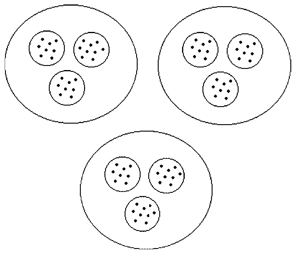
Schematic view of a hierarchical system. The system shown is composed of three groups that are themselves divided into three subgroups. The interactions within a group are strong and the interactions between the groups are weak.

In order to emphasize the hierarchical structure of the system, (1) is rewritten as follows:

\frac{d n_{j}^{α}}{d τ} = f_{j}^{α} (n^{α}) + ϵ \cdot \sum_{\begin{matrix} β = 1 \\ β \neq α \end{matrix}}^{A} f_{j}^{α β} (n^{α}, n^{β}) for α \in {1, 2, \dots, A} and j \in {1, 2, \dots, N^{α}}

(2)

where

n^{α} = (n_{1}^{α}, n_{2}^{α}, \dots, n_{N^{α}}^{α})

, ε is a dimensionless parameter and τ is the fast time unit.

The (intra-group) part f_j^α of the differential equations, which contains only variables belonging to the group α of the particular variable n_j^α, has been separated from the remaining (inter-group) part, which includes the coupling with the other groups. The basic assumption that defines a hierarchical system is that the intra-group part is much larger than the inter-group part, i.e., that the parameter ε is small. In other words, in a hierarchical system the interactions within a group are strong while the coupling between different groups is weak. As a consequence, the inter-group part in system (2) can be regarded as perturbations with respect to the intra-group one.

3 Choice of global variables

An important step in the aggregation method is to introduce for each group α a global variable V^α. V^α is a function of n_j^α and the dynamics of V^α is expressed in terms of n_j^α as:

\frac{d V^{α}}{d τ} = \sum_{j = 1}^{N^{α}} \frac{\partial V^{α}}{\partial n_{j}^{α}} \cdot \frac{d n_{j}^{α}}{d τ} for α \in {1, 2, \dots, A}

(3)

and introducing equations (2):

\frac{d V^{α}}{d τ} = I + ϵ \cdot E for α \in {1, 2, \dots, A}

(4)

where

I = \sum_{j = 1}^{N^{α}} \frac{\partial V^{α}}{\partial n_{j}^{α}} \cdot f_{j}^{α} (n^{α})

(5)

describes the dynamics due to internal effects and

E = \sum_{\begin{matrix} β = 1 \\ β \neq α \end{matrix}}^{A} \sum_{j = 1}^{N^{α}} \frac{\partial V^{α}}{\partial n_{j}^{α}} \cdot f_{j}^{α β} (n^{α}, n^{β})

(6)

describes the role of variables external to the group.

The global variables V^α have to be chosen in such a way that their dynamics is slow with respect to that of the intra-group variables n_j^α. An efficient way to define these variables is to look for conserved quantities for the intra-group dynamics, i.e., quantities that would remain constant if the inter-group interaction was turned off. The mathematical consequence for the choice of such variables is that the internal part vanishes, i.e., I=0. Consequently, the dynamics of the variables V^α is only governed by the slow part E of the complete system. It is therefore convenient to introduce a slow time unit t=ε·τ. Then, at the slow time scale, the system (4) becomes:

\frac{d V^{α}}{d t} = E for α \in {1, 2, \dots, A}

(7)

4 The aggregated model

The last step of the aggregation method is to express E in terms of the global variable V^α only. A sufficient condition is that the fast part dynamics quickly reaches an asymptotically stable equilibrium, denoted $n^{α^{*}}$ . For every α, $n^{α^{*}}$ is the equilibrium of the complete system (2) when ε is set to 0. $n^{α^{*}}$ is a function of V^α (constant at the fast time scale), which can be substituted into equations (7) leading to the following system for the global variables:

\frac{d V^{α}}{d t} = \sum_{\begin{matrix} β = 1 \\ β \neq α \end{matrix}}^{A} \sum_{j = 1}^{N^{α}} \frac{\partial V^{α}}{\partial n_{j}^{α}} (V^{α}) \cdot f_{j}^{α β} (V^{1}, V^{2}, \dots, V^{A}) for α \in {1, 2, \dots, A}

(8)

This method has been extended to systems where the fast part dynamics shows a stable limit cycle [22] and in some cases of infinite dimensional dynamical systems (systems of partial derivative equations) [23,24].

In system (8), the dynamics of each global variable V^α depends on global variables only: this system is called the aggregated model. The aggregated model is a set of A equations only while the complete system (2) is composed of N equations. For instance, in the case of a partition into three groups, each one containing three subgroups, like in Fig. 1, we get three global equations in (8) instead of nine equations in (2). This clearly shows how this method can lead to an important reduction in the number of equations.

An aggregated model is different from the initial complete model. However, it can be shown that the dynamics of the aggregated model is a good approximation of the dynamics of the complete one if (i) ε is small enough and (ii) the aggregated model is structurally stable. If the second proposal does not hold, one has to calculate further terms of the aggregated model that can be expressed as a Taylor expand in function of increasing powers of the small parameter ε [13,14,16].

5 Applications to population dynamics

In the context of population dynamics, the state variables n_j^α are population densities. For instance, index j refers to different spatial patches and index α to different species. The intra-group dynamics is the migration between the patches for each species, which is conservative; the inter-group dynamics is the interaction between the species. The global variables V^α=∑_j=1^{N^α}n_j^α are the total populations per species, the partial derivatives of the global variables are simply $\frac{\partial V^{α}}{\partial n_{j}^{α}} = 1$ for any α and j, and system (8) simplifies:

\frac{d V^{α}}{d t} = \sum_{\begin{matrix} β = 1 \\ β \neq α \end{matrix}}^{A} \sum_{j = 1}^{N^{α}} f_{j}^{α β} (V^{1}, V^{2}, \dots, V^{A}) for α \in {1, 2, \dots, A}

(9)

In order to illustrate the general method, we are now going to present a new and original application to population dynamics. We consider a population that is distributed on two spatial patches. Let n₁(t) and n₂(t) be, respectively, the sub-populations densities on patch 1 and 2 at time t. The complete model is composed of the two following equations:

{\begin{matrix} ϵ \frac{d n_{1}}{d t} = (k_{12} n_{2} - k_{21} n_{1}) + ϵ r_{1} n_{1} (n_{1} - M) (K - n_{1}) \\ ϵ \frac{d n_{2}}{d t} = (k_{21} n_{1} - k_{12} n_{2}) + ϵ r_{2} n_{2} \end{matrix}

(10)

where all parameters are positive, K>M and ε is a small positive dimensionless parameter.

The model is composed of two components, a fast part corresponding to migrations between the two patches and a slow part that relates to the sub-population growth on each patch. The fast part describes the migration between the two patches with constant migration rates k_ij from patch j to patch i. Imagine that the two patches would not be connected, i.e., the migration rates are equal to zero. Then sub-population dynamics on patch 1 would show an Allee effect [25]: for any positive initial condition below the threshold M, the population would decay and go to extinction; otherwise it would tend to the carrying capacity K. Patch 2 would be a source or a sink according to the sign of the growth rate r₂. We now study the situation where the two patches are connected by fast migration. In this case, the aggregation method presented above can be applied. First, it is easy to show that the fast part has a positive and asymptotically stable equilibrium: (11)

where the constants

ν_{i}^{*}

represent the proportions of individuals on patch i, i∈{1,2}, at the fast equilibrium, and n(t)=n₁(t)+n₂(t) is the total population density. Substitution of the fast equilibrium into the complete model leads to the following aggregated model governing the total population:

\frac{d n}{d t} = [r_{2} ν_{2}^{*} + r_{1} ν_{1}^{*} (ν_{1}^{*} n - M) (K - ν_{1}^{*} n)] n

(12)

Right-hand side of (12) is a polynomial equation of degree 3. Therefore, the model (12) can have one, two or three equilibria. The origin 0 is always equilibrium. Two more equilibria can occur according to the sign of

Δ = r_{1} {(ν_{1}^{*})}^{3} (r_{1} ν_{1}^{*} {(M - K)}^{2} + 4 r_{2} ν_{2}^{*})

There are three different cases.

(i) $r_{2} < - \frac{r_{1} ν_{1}^{*} {(M - K)}^{2}}{4 (1 - ν_{1}^{*})}$ . This condition is equivalent to Δ<0. The origin is the unique equilibrium and it is asymptotically stable. The total population goes to extinction (Fig. 2A): the global dynamics is sink-like.
(ii) $- \frac{r_{1} ν_{1}^{*} {(M - K)}^{2}}{4 (1 - ν_{1}^{*})} < r_{2} < \frac{r_{1} ν_{1}^{*} MK}{1 - ν_{1}^{*}}$ . This condition implies that Δ>0. There exist three equilibria, the origin (stable) and two positive ones, the smallest being unstable and the largest stable (Fig. 2B). In this case, the global dynamics shows an Allee effect.
(iii) $r_{2} > \frac{r_{1} ν_{1}^{*} MK}{1 - ν_{1}^{*}}$ . This condition implies that Δ>0. There exist three equilibria, the origin and two others, one positive and one negative. The origin is unstable and the positive equilibrium is stable. Thus, the global dynamics is logistic-like (Fig. 2C).

Fig. 2
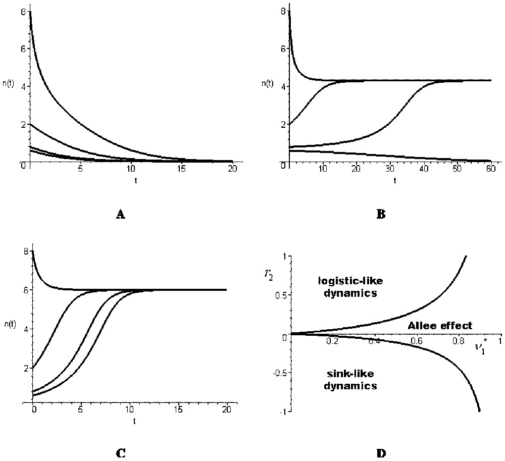
(A)–(C) Time evolution of the total population density in the aggregated model (12) with r₁=0.2, M=0.5, K=2, $ν_{1}^{*} = 0.5$ , $ν_{2}^{*} = 1 - ν_{1}^{*} = 0.5$ and (A) r₂=−0.5, (B) r₂=0.05, (C) r₂=0.5. (D) The three types of dynamics shown by the aggregated model [12] with respect to $ν_{1}^{*}$ and r₂ (the curves shown correspond to the particular values of the parameters r₁=0.2, M=0.5 and K=2, but their shapes are general).

The three previous cases are represented on Fig. 2D with respect to parameters $ν_{1}^{*}$ and r₂. In the sink-like and Allee effect cases, the total population has a global behaviour that is similar to the local behaviour of one of its sub-populations. However, in the logistic-like case, the total population behaviour is different from its sub-populations behaviours. This example shows that, in general, the global model may have a qualitatively different dynamics than the local ones.

Regarding other applications to population dynamics, aggregation methods have been used in the following cases: (i) modelling a trout fish population in an arborescent river network composed of patches connected by fast migration [26,27]; (ii) studying the effects of different individual decisions on the global dynamics of a prey-predator system in an heterogeneous environment composed of patches connected by fast migration [28–32]; (iii) modelling a sole larvae population with a continuous age with fast migration between different spatial patches [23]; (iv) modelling the influence of different individual strategies on the dynamics of a population of two competing populations using fast game dynamics [33–36]; (v) studying the effect of frequent migrations on the stability and persistence of host–parasitoid systems [37].

6 Conclusion

Starting from a complex dynamical system, the aggregation method presented in this paper enables to build a reduced system which dynamics is easier to analyse. This method relies on the existence of different time scales, i.e., the dynamics of the system involves fast and slow components. Then, the method allows to investigate the effects of the fast processes on the slow dynamics and reciprocally.

The method is general and can be applied in many contexts where hierarchical dynamical systems are used, i.e., in most fields of biology and ecology. Molecular biology made recent important improvements in understanding biological processes at the microscopic level. The next challenge is to develop an integrative approach to assess the influences of these processes at a macroscopic level. In this perspective, aggregation methods can be used as they are based on mutual dependence of the intra- and inter-level dynamics.

Bibliographie

[1] H.H. Pattee Hierarchy Theory: The Challenge of Complex Systems, George Braziller, New York, 1973

[2] H.A. Simon The Sciences of the Artificial, MIT Press, Cambridge, UK, 1969

[3] P. Weiss Hierarchically Organized Systems in Theory and in Practise, Hafner Publishing Company, New York, 1971

[4] T.F.H. Allen; T.B. Starr Hierarchy. Perspectives for Ecological Complexity, University of Chicago, Chicago, 1982

[5] P. Auger Dynamics and Thermodynamics in Hierarchically Organized Systems, Pergamon Press, Oxford, UK, 1989

[6] S. Muratori; S. Rinaldi Low- and high-frequency oscillations in three-dimensional food chain systems, SIAM J. Appl. Math., Volume 52 (1992), pp. 1688-1706

[7] S. Rinaldi; S. Muratori Limit cycles in slow–fast-pest models, Theor. Popul. Biol., Volume 41 (1992), pp. 26-43

[8] S. Rinaldi; S. Muratori Slow–fast limit cycles in predator-prey models, Ecol. Model., Volume 61 (1992), pp. 287-308

[9] Y. Iwasa; V. Andreasen; S.A. Levin Aggregation in model ecosystems. I. Perfect aggregation, Ecol. Model., Volume 37 (1987), pp. 287-302

[10] Y. Iwasa; S.A. Levin; V. Andreasen Aggregation in model ecosystems. II. Approximate aggregation, IMA J. Math. Appl. Med., Volume 6 (1989), pp. 1-23

[11] S. Levin; S. Pacala Theories of simplification and scaling of spatially distributed processes (D. Tilman; P. Kareiva, eds.), Spatial Ecology: The Role of Space in Population Dynamics and Interspecific Interactions, Princeton University Press, Princeton, USA, 1997, pp. 204-232

[12] S. Pacala; S.A. Levin Biologically generated spatial patterns and the coexistence of competing species (D. Tilman; P. Kareiva, eds.), Spatial Ecology: The Role of Space in Population Dynamics and Interspecific Interactions, Princeton University Press, Princeton, USA, 1997, pp. 271-295

[13] P. Auger; R. Roussarie Complex ecological models with simple dynamics: from individuals to populations, Acta Biotheor., Volume 42 (1994), pp. 111-136

[14] P. Auger; J.-C. Poggiale Emergence of population growth models: fast migration and slow growth, J. Theor. Biol., Volume 182 (1996), pp. 99-108

[15] P. Auger; J.-C. Poggiale Aggregation and emergence in systems of ordinary differential equations, Math. Comput. Model., Volume 27 (1998), pp. 1-21

[16] J.-C. Poggiale, Applications des variétés invariantes à la modélisation de l'hétérogénéité en dynamique de populations, PhD Thesis, Dijon, 1994

[17] R. Bravo de la Parra; P. Auger; E. Sànchez Aggregation methods in discrete models, J. Biol. Syst., Volume 3 (1995), pp. 603-612

[18] R. Bravo de la Parra; E. Sànchez; O. Arino; P. Auger A discrete model with density dependent fast migration, Math. Biosci., Volume 157 (1999), pp. 91-110

[19] E. Sànchez; R. Bravo de la Parra; P. Auger Discrete models with different timescales, Acta Biotheor., Volume 43 (1995), pp. 465-479

[20] L. Sanz, Métodos de agregacion en sistemas discretos, PhD thesis, Madrid, 1998

[21] L. Sanz; R. Bravo de la Parra Variables Aggregation in a time-discrete linear model, Math. Biosci., Volume 157 (1999), pp. 111-146

[22] J.-C. Poggiale; P. Auger Fast oscillating migrations in a prey–predator model, Math. Mod. Meth. Appl. S., Volume 6 (1995), pp. 217-226

[23] O. Arino; E. Sànchez; R. Bravo de la Parra; P. Auger A singular perturbation in an age-structured population model, SIAM J. Appl. Math., Volume 60 (1999), pp. 408-436

[24] R. Bravo de la Parra; O. Arino; E. Sànchez; P. Auger A model of an age-structured population with two time scales, Math. Comput. Model., Volume 31 (2000), pp. 17-26

[25] A. Bazykin Nonlinear Dynamics of Interacting Populations, World Scientific Series on Nonlinear Science, Series A, 11, World Scientific, 1998

[26] S. Charles; R. Bravo de la Parra; J.-P. Mallet; H. Persat; P. Auger Population dynamics modelling in an hierarchical arborescent river network: an attempt with Salmo trutta, Acta Biotheor., Volume 46 (1998), pp. 223-234

[27] S. Charles; R. Bravo de la Parra; J.-P. Mallet; H. Persat; P. Auger A density-dependent model describing Salmo trutta population dynamics in an arborescent river network: effects of dams and channelling, C. R. Acad. Sci. Paris, Ser. III (1998), pp. 979-990

[28] P. Auger; S. Charles; M. Viala; J.-C. Poggiale Aggregation and emergence in ecological modelling: integration of ecological levels, Ecol. Model., Volume 127 (2000), pp. 11-20

[29] C. Bernstein; P. Auger; J.-C. Poggiale Predator migration decisions, the ideal free distribution and predator-prey dynamics, Am. Nat., Volume 153 (1999), pp. 267-281

[30] G. Chiorino; P. Auger; J.-L. Chassé; S. Charles Behavioral choices based on patch selection: a model using aggregation methods, Math. Biosci., Volume 157 (1999), pp. 189-216

[31] J. Michalski; J.-C. Poggiale; R. Arditi; P. Auger Effects of migration modes on predator–prey systems in patchy environments, J. Theor. Biol., Volume 185 (1997), pp. 459-474

[32] J.-C. Poggiale; J. Michalski; R. Arditi Emergence of donor control in patchy predator–prey systems, Bull. Math. Biol., Volume 60 (1998), pp. 1149-1166

[33] P. Auger; D. Pontier Fast game theory coupled to slow population dynamics: the case of domestic cat populations, Math. Biosci., Volume 148 (1998), pp. 65-82

[34] E. Sànchez; P. Auger; R. Bravo de la Parra Influence of individual aggressiveness on the dynamics of competitive populations, Acta Biotheor., Volume 45 (1997), pp. 321-333

[35] D. Pontier; P. Auger; R. Bravo de la Parra; E. Sànchez The impact of behavioral plasticity at individual level on domestic cat population dynamics, Ecol. Model., Volume 133 (2000), pp. 117-124

[36] P. Auger; R. Bravo de la Parra; E. Sànchez Behavioral dynamics of two interacting hawk-dove populations, Math. Mod. Meth. Appl. S., Volume 11 (2001), pp. 645-661

[37] C. Lett; P. Auger; R. Bravo de la Parra Migration frequency and the persistence of host–parasitoid interactions, J. Theor. Biol., Volume 221 (2003), pp. 639-654

Commentaires - Politique