Impact of spatial heterogeneity on a predator–prey system dynamics

Jean-Christophe Poggiale; Pierre Auger

doi:10.1016/j.crvi.2004.06.006

Biological modelling / Biomodélisation

Impact of spatial heterogeneity on a predator–prey system dynamics
[Impact de l'hétérogénéité spatiale sur la dynamique d'un système prédateur–proie.]

Présenté par : Pierre Auger

Jean-Christophe Poggiale ¹ ; Pierre Auger ²

¹ Centre d'océanologie de Marseille, UMR 6117, campus de Luminy-Case 901, 13288 Marseille cedex 9, France
² UMR 5558, université Claude-Bernard, Lyon 1, 69622 Villeurbanne cedex, France

Comptes Rendus. Biologies, Volume 327 (2004) no. 11, pp. 1058-1063.

Résumés

Anglais
Français

This paper deals with the study of a predator–prey model in a patchy environment. Prey individuals moves on two patches, one is a refuge and the second one contains predator individuals. The movements are assumed to be faster than growth and predator–prey interaction processes. Each patch is assumed to be homogeneous. The spatial heterogeneity is obtained by assuming that the demographic parameters (growth rates, predation rates and mortality rates) depend on the patches. On the predation patch, we use a Lotka–Volterra model. Since the movements are faster that the other processes, we may assume that the frequency of prey and predators become constant and we would get a global predator–prey model, which is shown to be a Lotka–Volterra one. However, this simplified model at the population level does not match the dynamics obtained with the complete initial model. We explain this phenomenom and we continue the analysis in order to give a two-dimensional predator–prey model that gives the same dynamics as that provided by the complete initial one. We use this simplified model to study the impact of spatial heterogeneity and movements on the system stability. This analysis shows that there is a globally asymptotically stable equilibrium in the positive quadrant, i.e. the spatial heterogeneity stabilizes the equilibrium.

Dans cet article, nous étudions un système prédateur–proie dans un environnement divisé en deux sites. Les proies se déplacent sur les deux sites, l'un étant un refuge et l'autre contenant des prédateurs. Les déplacements sont supposés plus rapides que la croissance et que les processus de prédation. Chaque site est supposé homogène. L'hétérogénéité spatiale est obtenue en supposant que les paramètres démographiques (taux de croissance et taux de mortalité) dépendent du site. Sur le site de prédation, on utilise un modèle de Lotka–Volterra. Comme les déplacements sont plus rapides que les autres processus, on peut supposer que les proportions de proie sur chaque site deviennent rapidement constantes, ce qui, comme nous le montrons, conduit à un modèle global prédateur–proie de type Lotka–Volterra. Cependant, ce modèle simplifié à l'échelle des populations globales ne fournit pas la même dynamique que celle obtenue avec le modèle initial. Nous expliquons ce phénomène et nous poursuivons notre analyse pour construire un modèle à deux équations gouvernant les abondances de populations totales et qui donne la même dynamique que celle obtenue avec le modèle complet initial. Nous utilisons alors ce modèle simplifié pour étudier l'impact de l'hétérogénéité spatiale, ainsi que celui des déplacements, sur la stabilité du système. Cette analyse montre qu'il existe un équilibre globalement asymptotiquement stable dans le quadrant positif, autrement dit, que l'hétérogénéité a pour conséquence une stabilisation du système.

Métadonnées

Reçu le : 2004-01-27
Accepté le : 2004-06-09
Publié le : 2004-11-01

PMID

DOI : 10.1016/j.crvi.2004.06.006

Keywords: Lotka–Volterra, predator–prey model, aggregation methods, spatial heterogeneity, stability
Mot clés : Lotka–Volterra, prédateur–proie, méthodes d'agrégation, hétérogénéité spatiale, stabilité

Affiliations des auteurs :

Jean-Christophe Poggiale ¹ ; Pierre Auger ²

¹ Centre d'océanologie de Marseille, UMR 6117, campus de Luminy-Case 901, 13288 Marseille cedex 9, France
² UMR 5558, université Claude-Bernard, Lyon 1, 69622 Villeurbanne cedex, France

@article{CRBIOL_2004__327_11_1058_0,
     author = {Jean-Christophe Poggiale and Pierre Auger},
     title = {Impact of spatial heterogeneity on a predator{\textendash}prey system dynamics},
     journal = {Comptes Rendus. Biologies},
     pages = {1058--1063},
     publisher = {Elsevier},
     volume = {327},
     number = {11},
     year = {2004},
     doi = {10.1016/j.crvi.2004.06.006},
     language = {en},
}

TY  - JOUR
AU  - Jean-Christophe Poggiale
AU  - Pierre Auger
TI  - Impact of spatial heterogeneity on a predator–prey system dynamics
JO  - Comptes Rendus. Biologies
PY  - 2004
SP  - 1058
EP  - 1063
VL  - 327
IS  - 11
PB  - Elsevier
DO  - 10.1016/j.crvi.2004.06.006
LA  - en
ID  - CRBIOL_2004__327_11_1058_0
ER  -

%0 Journal Article
%A Jean-Christophe Poggiale
%A Pierre Auger
%T Impact of spatial heterogeneity on a predator–prey system dynamics
%J Comptes Rendus. Biologies
%D 2004
%P 1058-1063
%V 327
%N 11
%I Elsevier
%R 10.1016/j.crvi.2004.06.006
%G en
%F CRBIOL_2004__327_11_1058_0

Jean-Christophe Poggiale; Pierre Auger. Impact of spatial heterogeneity on a predator–prey system dynamics. Comptes Rendus. Biologies, Volume 327 (2004) no. 11, pp. 1058-1063. doi : 10.1016/j.crvi.2004.06.006. https://comptes-rendus.academie-sciences.fr/biologies/articles/10.1016/j.crvi.2004.06.006/

Version originale du texte intégral

1 Introduction

The role of spatial heterogeneity and migrations on predator–prey or host–parasite systems stability has been studied in many papers. In [1], the authors exhibit the stabilizing effect of migrations in a spatially distributed host–parasite system. Some authors have then investigated the impact of density dependence in the migration processes on the predator–prey interactions stability (see [2–7], for instance). Even if the initial works have shown that the spatial heterogeneity and the migrations should stabilize the systems, Murdoch and Oaten [8] studied a system exhibiting the opposite effect. It followed a series of papers dealing with the impact of spatial heterogeneity on predator–prey (or host–parasitoid) systems' stability and the main conclusion was that the stability of the system depends on the details included in the models.

In the previous works, the interactions models had either asymptotically stable or unstable equilibria. For instance, in [7], the model is a two patches host–parasitoid system with a linear growth function for the host on each patch, a Holling type-II functional response on each patch and a linear decay for the parasitoid in the absence of host on each patch. In this kind of system, the positive equilibrium is known to be unconditionnally unstable. The density-dependent migration rates used by the author can stabilize the equilibrium. However, it is difficult to quantify exactly which part of the density dependence in the rates, which part of the spatial heterogeneity, and which part of the interaction processes contribute to the stabilization. In the present work, we expect that the choice of a neutrally stable model for the interaction part and constant migration rates should give a best insight into the understanding of the role of spatial heterogeneity on stabilization of predator–prey models.

Indeed, we consider a predator–prey model on two patches. One patch is a refuge for the prey, thus there is no predator in this patch. On the second patch, we used a Lotka–Volterra model to describe the interactions. This choice is governed by the stability property of this model: the positive equilibrium is neutrally stable. In this case, the interactions part do not contribute neither to stabilization nor to unstabilization. For the migrations, we used constant rates in order to eliminate any effect of density dependence. Since the interaction part is neutral from the stability point of view, all the stabilization effects are contained only in the migration processes and in the spatial heterogeneity. Moreover, we can easily admit that a good choice of the density dependence function used for the migration rates can compensate the terms generating the unstability. Since we have chosen density-independent migration rates, the stabilization is just the result of spatial heterogeneity.

In order to deal with the three-dimensional system, we use a time scale arguments which allows us to consider only the total populations densities, that is a two-dimensional system. This kind of methods has been described for instance in [9–11]. Our approach can be compared in a first approximation to the so-called ‘quasi-steady-state’ assumption. However, we show in the particular model of this paper that the later method is not sufficient and that the former can be used. The obtained two-dimensional system is a perturbation of the Lotka–Volterra model. This famous model is not structurally stable and our analysis shows that the perturbation ‘breaks’ the closed curves. In fact, for the complete initial model, there exists a two-dimensional invariant attracting manifold. The aggregated model is the restriction of the complete system to this invariant manifold. In practice, the invariant manifold is obtained by the use of a Taylor expansion with respect to a small parameter (the time scale factor). In the first approximation, the reduced model is of Lotka–Volterra type. Thus we need to continue the analysis by computing the second term in the expansion.

Finally, we prove that there is a unique equilibrium with positive coordinates and that this equilibrium is globally asymptotically stable, for all the parameter values. Thus the spatial heterogeneity has a stabilizing effects on the predator–prey interactions. Furthermore, there is no possible bifurcation on the invariant manifold, thus the previous result is complete.

The plan of this article is as follows: we first describe the complete predator–prey model, the following section explain how the reduced model is obtained. Then we analyse the reduced model and the last section provides a discussion on the results.

2 The complete model

We consider a predator–prey model on two patches. The prey can move on both patches while the predator remains on patch 1. The patch 2 is thus a refuge for the prey. We denote by $x_{i}$ the prey density on patch i, $i = 1, 2$ . We denote by y the predator density. On each patch, the prey population growth rate and the predator population death rate are linear, the predation rate is bilinear, that is proportional to prey and predator densities and the predator growth rate is proportional to the predation rate. The model is given by the following set of three ordinary differential equations:

\frac{d x_{1}}{d τ} = m_{2} x_{2} - m_{1} x_{1} + ɛ x_{1} (r_{1} - a y)

(1a)

\frac{d x_{2}}{d τ} = m_{1} x_{1} - m_{2} x_{2} + ɛ x_{2} r_{2}

(1b)

\frac{d y}{d τ} = ɛ y (b x_{1} - d)

(1c)

where

m_{i}

are respectively the proportions of prey populations leaving patch i by displacement per unit time,

r_{i}

is the prey population growth rate on patch i, d is the predator population death rate, a is the predation rate on patch and

b x_{1}

is the per capita predator growth rate.

ɛ ≪ 1

is a small parameter, which means that movements have a larger speed than that associated to growth and death processes.

Let $x = x_{1} + x_{2}$ be the total amount of prey population. It follows that $u_{1} = \frac{x_{1}}{x}$ and $u_{2} = \frac{x_{2}}{x}$ are the proportions of prey on patch 1 and patch 2, respectively. With these variables, we can write the system (1) in the following equivalent way:

\frac{d u_{1}}{d τ} = m_{2} - (m_{1} + m_{2}) u_{1} + ɛ u_{1} (1 - u_{1}) (r_{1} - r_{2} - a y)

(2a)

\frac{d x}{d τ} = ɛ x (r_{1} u_{1} + r_{2} u_{2} - a u_{1} y)

(2b)

\frac{d y}{d τ} = ɛ y (b u_{1} x - d)

(2c)

3 Reduction of the dimension

In this section, we build a two-dimensional system governing the dynamics of the total populations densities x and y. Morevover, this system gives the same dynamics as that obtained for x and y in the system (2). This will facilitate the mathematical study of system (1) provided in the next section.

The reduction method is based on the fact that the system (2) has two different typical time scales. From the mathematical point of view, the method is based on a theorem due separately to Hirsch, Pugh and Shub in [12] and Fenichel in [13]. The interested reader can find more informations in [14,15] or in [16], for instance, and in the references given within these works. The mathematical theorems provide a justification to a method that is often used on the basis of intuition: since variables are fast, after a short time, these variables are close to their equilibrium values (if they exist) and then we replace the fast variables by their equilibrium values in the differential equations governing the slow variables, leading to a differential system that has the same dimension as the number of slow variables. This method is sometimes called ‘quasi-steady-state assumption’ method and can be used to build trophic chain models [17] and to analyse them [18,19]. However, in some cases, like in the present work, the quasi-steady-state assumption is not sufficient to determine the dynamics of the slow variables and the mathematical theorems provide usefull results that permit to conclude on the dynamics. We will illustrate this on the model studied in this paper.

Let us start to calculate the fast equilibrium, that is the equilibrium value of the fast variable $u_{1}$ . In order to get this equilibrium value, we put $ɛ = 0$ in system (2). The result is:

u_{1}^{*} = \frac{m_{2}}{m_{1} + m_{2}} and u_{2}^{*} = \frac{m_{1}}{m_{1} + m_{2}}

(3)

By replacing

u_{i}

u_{i}^{*}

in (2b) and in (2c), we get the following two-dimensional system:

\frac{d x}{d t} = x (r - a_{1} y)

(4a)

\frac{d y}{d t} = y (b_{1} x - d)

(4b)

where

t = ɛ τ

r = r_{1} u_{1}^{*} + r_{2} u_{2}^{*}

a_{1} = a u_{1}^{*}

and

b_{1} = b u_{1}^{*}

The system (4) is a classical Lotka–Volterra model. All the solutions of this system with initial conditions in the positive quadrant are periodic. There is a positive equilibrium which is a centre. However, the dynamics of x and y in the system (2) does not match with the Lotka–Volterra dynamics, as illustrated in Fig. 1. Indeed, when we replace the fast variable by its equilibrium value, we make an error in the order of ɛ. Since the Lotka–Volterra model is not structurally stable, the ɛ-error can play an important role in the dynamics. The Fenichel theorem, for instance, claims that there is an invariant manifold $W$ defined by $u_{1} = u_{1} (x, y, ɛ)$ in the phase space $(u_{1}, x, y, ɛ)$ . Since the fast equilibrium is hyperbolically stable, the manifold $W$ is normally hyperbolically stable, that is a trajectory starting in the neigbourhood of $W$ is attracted with an exponential speed. The previous approximation we made is thus a zero-order approximation of this manifold.

Fig. 1
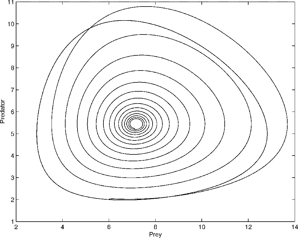
Comparison between the dynamics of x and y given by the complete system (1) and that obtained with the two-dimensional system (4). We see on this figure that the complete system exhibits a stable focus while with the reduced system, the trajectory is a closed curve. The parameters values used in the simulation are: $m_{1} = 2$ , $m_{2} = 1$ , $r_{1} = 1$ , $r_{2} = 2$ , a=1, d=2, b=0.9 and ɛ=0.05.

We can get a first-order approximation of the manifold in the following way. Let us write:

u_{1} (x, y, ɛ) = u_{1}^{*} + ɛ w_{1} (x, y) + o (ɛ)

(5)

We have to determine

w_{1}

and then to replace

u_{1}

by its expression (5) in the system (2) in order to improve the approximate two-dimensional model (4). We can note that the asymptotic expansion of the derivative

\frac{d u_{1}}{d τ}

with respect to the small parameter ɛ can be written in two different ways. The first one consists in replacing

u_{1}

by the expression (5) in Eq. (2a). The second way consists in writing:

\frac{d u_{1}}{d τ} = \frac{\partial u_{1}}{\partial x} \frac{d x}{d τ} + \frac{\partial u_{1}}{\partial y} \frac{d y}{d τ}

(6)

Then we identify the terms in the order of ɛ in both formulas, we get:

- (m_{2} + m_{1}) w_{1} (x, y) + u_{1}^{*} (1 - u_{1}^{*}) (r_{1} - r_{2} - a_{1} y) = 0

(7)

which allows us to conclude that

w_{1}

is a function depending only on y:

w_{1} (y) = \frac{u_{1}^{*} (1 - u_{1}^{*})}{m_{2} + m_{1}} (r_{1} - r_{2} - a_{1} y)

(8)

It follows that the system on the invariant manifold is reduced to:

\frac{d x}{d t} = x (r - a y) + ɛ x w_{1} (y) (r_{1} - r_{2} - a_{1} y)

(9a)

\frac{d y}{d t} = y (b x - d) + ɛ y b_{1} w_{1} (y) x

(9b)

A numerical simulation has been performed and is shown in Fig. 2, in order to illustrate that this reduced model provides a good approximation of the dynamics of the total population densities governed by the three-dimensional system (2). Since we get a two-dimensional system, the mathematical analysis is easier and we will perform it in the next section.

Fig. 2
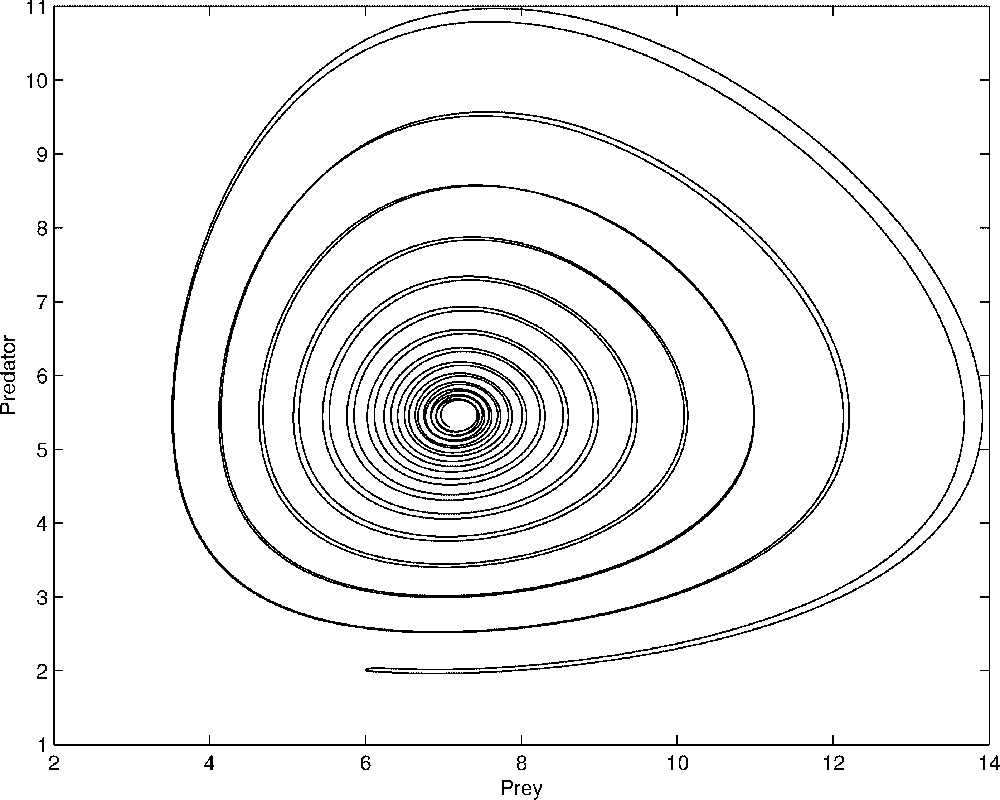
Comparison between the dynamics of x and y given by the complete system (1) and that obtained with the two-dimensional system (9). We see on this figure that the reduced system solution matches quite well the complete model solution. The parameters values used in the simulation are: $m_{1} = 2$ , $m_{2} = 1$ , $r_{1} = 1$ , $r_{2} = 2$ , a=1, d=2, b=0.9 and ɛ=0.05.

4 Mathematical analysis

In this section, the mathematical analysis of the system (9) is performed. We show that there is a globally asymptotic equilibrium in the positive quadrant and there is no bifurcation.

Let us denote by X the vector field associated to the system (9) and let $\tilde{X}$ be the vector field $\frac{X}{x y}$ defined on ${x > 0; y > 0}$ . We denote by $ω_{ɛ}$ the dual form associated with $\tilde{X}$ . We can clearly write:

ω_{ɛ} (x, y) = d H (x, y) + ɛ η (x, y)

(10)

where

H (x, y) = b_{1} x - d \ln x + a_{1} y - r \ln y + C

(11)

C is a constant, and

η (x, y) = b w_{1} (x, y) d x - w_{1} (x, y) (\frac{r_{1} - r_{2}}{y} - a) d y

(12)

We know that for

ɛ = 0

, there is a unique equilibrium in the positive quadrant and that this equilibrium is a centre. It is a straighforward consequence of the implicit function theorem that there is also an equilibrium in the positive quadrant for small enough values of ɛ. Furthermore, we can define a return map (Poincaré map) on a half straight line by the equilibrium point, see Fig. 3. Let

δ (h) = P (h) - h

, the sign of δ gives an information on the equilibrium stability, and on the existence of limit cycles: if there is an h for which

δ (h) = 0

, then the trajectory by h is a closed curve corresponding to a periodic orbit. Let us denote by

Γ_{ɛ}

the trajectory defined by (9) and contained between the point h and the point

P (h)

, see Fig. 3. We can write the following equalities (Poincaré lemma):

δ (h) = \int_{Γ_{ɛ}} d H = \int_{Γ_{ɛ}} (ω_{ɛ} - ɛ η) = - ɛ \int_{Γ_{ɛ}} η = - ɛ \int_{{H = h}} η + o (ɛ)

(13)

Let

I = \int_{{H = h}} η

, if ɛ is small enough, the sign of

δ (h)

is the same as that of I. From the Stockes theorem, we have:

I = - \underset{{H ⩽ h}}{\int \int} d η = - \underset{{H ⩽ h}}{\int \int} \frac{a b u_{1}^{*} (1 - u_{1}^{*})}{m_{1} + m_{2}} d x \land d y = - \frac{a b u_{1}^{*}}{m_{1} + m_{2}} A (h) < 0

(14)

where

A (h)

is the area of the domain

{H ⩽ h}

Fig. 3
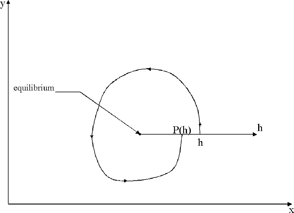
Scheme of the return map (Poincaré map) defined for an ɛ-perturbation of a centre. A half straight line is chosen, starting from the equilibrium point. This line is parameterised by a real number h. For each point h on this line, there is a trajectory defined by the system (9), leaving the line and coming back after turning around the equilibrium. The new contact with the line defines the map P(h). If P(h)<h, then the considered trajectory is going to the equilibrium, while if P(h)>h, the trajectory is going away from the equilibrium.

Since $δ (h) < 0$ for small enough ɛ values and for all h, it results that the equilibrium point is globally asymptotically stable.

5 Conclusion–discussion

A Lotka–Volterra model on two patches has been analysed. One of the patch is a refuge for the prey. This is a way to consider spatial variability. Morevover, the prey growth rates can be different on each patch. In the refuge, the prey has a constant growth rate. It means that if there were no displacement, the prey density would become larger and larger, going to infinity. The first consequence of the displacement is thus a control of the prey density by the predator. Moreover, on the predation patch, the dynamics should be periodic if the displacement were eliminated, since on this patch we considered a Lotka–Volterra model. The equilibrium point should be neutrally stable in that case. We shown that the complete model leads to a globally asymptotic equilibrium. This means that the spatial variability leads to a stabilisation of the dynamics. Even if it is a common result, it is the first time that it is obtained with a mathematical model having appropriate mathematical properties: neutral dynamics on the homogeneous patches and density-independent migration rates. This is the reason why we think that it is a robust result.

More precisely, we can see on Eq. (14) that the larger a, b and $u_{1}^{*} (1 - u_{1}^{*})$ are, the more stable the equilibrium is. In other words, when these parameters increase, the trajectories reach the equilibrium faster. a is the predation rate, then a stronger predation leads to a stronger stability. b is the predator growth rate per prey eaten, then a more efficient predator leads to a stronger stability. Finally, $u_{1}^{*}$ is the proportion of prey available for the predators and $u_{1}^{*} (1 - u_{1}^{*})$ takes the greatest value when $u_{1}^{*} = 1 / 2$ , that is when the prey is uniformally distributed on the patches: a half in the refuge, the other half in the predation patch. This spatial distribution leads to a stronger stability. We can thus conclude that the spatial heterogeneity plays a crucial role in the stabilization, but nor because it could permit the prey to avoid predation, neither because it could enhance the predation. This stabilization is mainly the result of the refuge.

Indeed, if we considered the same kind of model with the predator on both patches (with different rates on each patch), that is without any refuge for the prey, the result would be less obvious. This is the object of a future work.

Bibliographie

[1] M.P. Hassel; R.M. May Stability in insect host–parasite models, J. Anim. Ecol., Volume 42 (1973), pp. 693-726

[2] J.C. Allen Mathematical models of species interactions in time and space, Am. Nat., Volume 109 (1975), pp. 319-342

[3] P.H. Crowley Dispersal and the stability of predator–prey interactions, Am. Nat., Volume 118 (1981), pp. 673-701

[4] P. Chesson; W.W. Murdoch Aggregation of risk: relationship among host–parasitoid models, Am. Nat., Volume 127 (1986), pp. 697-715

[5] J. Reeve Environmental variability, migration and persistence in host–parasitoid systems, Am. Nat., Volume 118 (1988), pp. 810-836

[6] F.R. Adler Migration alone can produce persistence of host–parasitoid models, Am. Nat., Volume 141 (1993), pp. 642-650

[7] A.R. Ives Density-dependent and density-independent parasitoid aggregation in model host–parasitoid systems, Am. Nat., Volume 140 (1992), pp. 912-937

[8] W.W. Murdoch; A.S. Oaten Aggregation by parasitoids and predators: effects on equilibrium and stability, Am. Nat., Volume 134 (1989), pp. 288-310

[9] P. Auger; J.-C. Poggiale Emergence of population growth models: fast migrations and slow growth, J. Theor. Biol., Volume 182 (1996), pp. 99-108

[10] J.-C. Poggiale; P. Auger; R. Roussarie Perturbations of the classical Lotka–Volterra system by behavioural sequences, Acta Biotheor., Volume 43 (1995), pp. 27-39

[11] C. Bernstein; P. Auger; J.-C. Poggiale Predator migration decisions, the ideal free distribution and predator–prey dynamics, Am. Nat., Volume 153 (1999), pp. 267-281

[12] M.W. Hirsch; C.C. Pugh; M. Shub Invariant manifolds, Bull. Am. Math. Soc., Volume 76 (1970), pp. 1015-1019

[13] N. Fenichel Persistence and smoothness of invariant manifolds for flows, Indiana Univ. Math. J., Volume 21 (1971), pp. 193-226

[14] C.K.R.T. Jones Geometric singular perturbation theory (R. Johnson, ed.), Dynamical Systems, Montecatini Terme, Lecture Notes in Math., vol. 1609, 1994, pp. 44-118

[15] K. Sakamoto Invariant manifolds in singular perturbation problems for ordinary differential equations, Proc. R. Soc. Edinb. A, Volume 116 (1992), pp. 45-78

[16] S. Wiggins Normally hyperbolic invariant manifolds in dynamical systems, Appl. Math. Sci. Ser., Volume 105 (1994)

[17] R. Dilao; T. Domingos A general approach to the modelling of trophic food chains, Ecol. Model., Volume 132 (2000), pp. 191-202

[18] O. De Feo; S. Rinaldi Singular homoclinic bifurcations in tritrophic food chains, Math. Biosci., Volume 148 (1998), pp. 7-20

[19] Yu.A. Kuznetsov; O. De Feo; S. Rinaldi Belyakov homoclinic bifurcations in a tritrophic food chain model, SIAM J. Appl. Math., Volume 62 (2001), pp. 462-487

Commentaires - Politique

Ces articles pourraient vous intéresser

Bifurcations of a predator-prey model with non-monotonic response function

H.W. Broer; Vincent Naudot; Robert Roussarie; ...

C. R. Math (2005)

Does mutual interference always stabilize predator–prey dynamics? A comparison of models

Roger Arditi; Jean-Marc Callois; Yuri Tyutyunov; ...

C. R. Biol (2004)

Permanence of a stage-structured predator-prey system with a class of functional responses

Zhihui Ma; Shufan Wang; Wenting Wang; ...

C. R. Biol (2011)